A Distributed Indexing Method for Timeline Similarity Query


1
School of Computer Science, China University of Geosciences (Wuhan), 388 Lumo Road, Wuhan 430074, China
2
Department of Computer Science, University of Idaho, 875 Perimeter Drive MS 1010, Moscow, ID 83844-1010, USA
*
Author to whom correspondence should be addressed.
Algorithms 2018, 11(4), 41; https://doi.org/10.3390/a11040041
Submission received: 10 February 2018
/
Revised: 27 March 2018
/
Accepted: 29 March 2018
/
Published: 30 March 2018
Abstract
:Timelines have been used for centuries and have become more and more widely used with the development of social media in recent years. Every day, various smart phones and other instruments on the internet of things generate massive data related to time. Most of these data can be managed in the way of timelines. However, it is still a challenge to effectively and efficiently store, query, and process big timeline data, especially the instant recommendation based on timeline similarities. Most existing studies have focused on indexing spatial and interval datasets rather than the timeline dataset. In addition, many of them are designed for a centralized system. A timeline index structure adapting to parallel and distributed computation framework is in urgent need. In this research, we have defined the timeline similarity query and developed a novel timeline index in the distributed system, called the Distributed Triangle Increment Tree (DTI-Tree), to support the similarity query. The DTI-Tree consists of one T-Tree and one or more TI-Trees based on a triangle increment partition strategy with the Apache Spark. Furthermore, we have provided an open source timeline benchmark data generator, named TimelineGenerator, to generate various timeline test datasets for different conditions. The experiments for DTI-Tree’s construction, insertion, deletion, and similarity queries have been executed on a cluster with two benchmark datasets that are generated by TimelineGenerator. The experimental results show that the DTI-tree provides an effective and efficient distributed index solution to big timeline data.
1. Introduction
Timelines have been used for hundreds of years to represent sequences of interval events that may be biographies, historical summaries, or project plans. Most of them are often distilled as timelines to tell a story [1]. In recent years, almost every social media platform has a timeline tool, such as Facebook, Twitter, and Tencent. A large amount of data involving time is generated by their users’ devices especially smart phones on an unprecedented scale and speed. Those datasets can be organized by timelines for visualization and analysis. Every user can see clearly his or her friends’ activities displaying in their timelines. This is the common usage in social media platform. Another potential usage is to apply timeline similarities for friends, activities, or some products recommendation. All kinds of the usages of timelines need a powerful timeline index on a distributed platform.
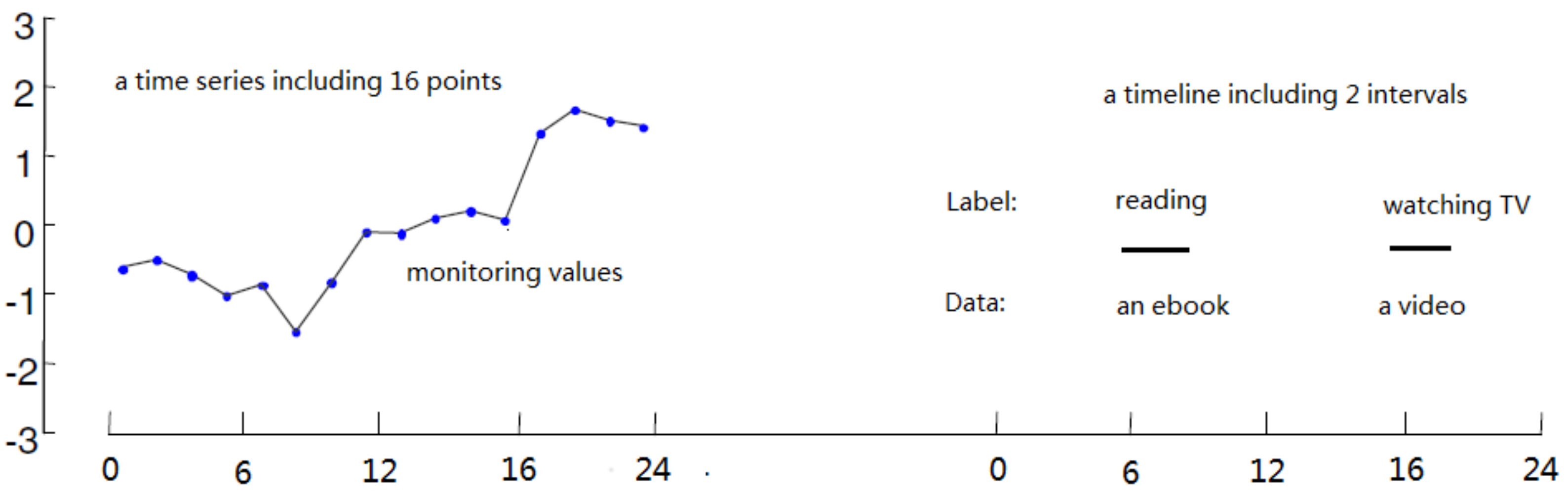
A timeline describes a series of interval event data, which is to be different from continuous quantitative time-series data [1], as shown in Figure 1. The time series data are often sensor-making, for example, some monitoring values. There are a lot of excellent researches that are focused on indexing massive time series or data series [2,3,4,5]. Most of them are based on the Symbolic Aggregate approXimation (SAX) strategy of iSAX [2]. However, a timeline is often a set of interval objects with labels and data. It is often not continuous, but rather discrete and hard to be organized as SAX words.
In addition, the data volume of the timelines mainly concentrates on their labels and attachment data. The labels indicate the type of intervals that are contained by the timeline. The data is an attachment of the labeled interval. The data may be text, image, or some other row binary data. As demonstrated in Figure 2, China, Japan, and Korea are long period historical timelines. Timelines can also be short. As shown in Figure 3, T1, T2, and T3 are daily timelines for worker, researcher, and pupil, respectively. A timeline often indicates the types of events being represented, the number of events, the chronological time when they occurred in, the order in which they occurred, how long they lasted, and whether any of them met or overlapped. For instance, suppose that the timeline S in Figure 3 represents a standard healthy daily timeline. We want to know which timeline in the tree timelines of T1, T2, and T3 is the most like S. Perhaps we can tell the result is T3 at a glance, because there are more overlaps with same labels between S and T3. However, such manual comparison will be hard to accomplish while the dataset is large. Hence, we defined a timeline similarity function that is shown in next section to evaluate it. Not only the storage of big timeline dataset but also the similarity query of timelines requires effective and efficient access methods. However, none of the existing special index structures have dealt with such methods yet.
An alternative approach is to transform the timelines into intervals and then use interval indices. An interval stores a value that represents a span of measurement, such as time, distance, and temperature. Generally, it can be represented by two attributes: start value and end value. Interval is a fundamental data type for temporal, spatial, and scientific databases that are essential to solve the problem of representing temporal knowledge and reasoning arising in a wide range of disciplines [6,7,8,9], especially in computer science and geoinformatics [10,11]. Since the 1990s, research on interval data management has made significant progress in various aspects and many remarkable results have been reported, however, many challenges in this filed still remain [8,9,12,13]. According to the reference [8], the existing interval indexes, including the Time Index [14], Segment R-tree [15], PR-tree [16], Interval B-Tree [17], Snapshot index [18], Fully Persistent B+-tree [19,20], RI-tree [21,22], TD-Tree [8], TB-Tree [9], and the SHB+-tree [23], etc. can be categorized into four groups [8]. Most existing interval index methods are extensions of traditional B+-tree [24,25] or R-tree [26]. In general, the tree-like index structures are a kind of centralized data structure. They are hierarchical and are not efficient for parallel implementations due to high concurrency control cost [9,27,28]. How to transform the tree-like structure into linear structure effectively and efficiently is one of the key solutions to this problem. Another noteworthy issue is that most space partitioning indexes, such as TD-Tree and TB-Tree, often have a predefined space region for the root node. It limits the scalability to indexing dynamic interval data set.
However, the timeline data are extremely large when all of them are converted into intervals with labels, and the data processing needs more computation, where it exceeds the capacity of traditional centralized technologies that are mentioned above. Some efforts have been performed to handle large-scale data. MapReduce [29] and MapReduce-Merge are two useful programming paradigms to handle large-scale data. Hadoop GIS [30], SpatialHadoop [28], and ST-Hadoop [31] were proposed to adapt the traditional spatial index structure, such as Quad-Trees and R-trees for MapReduce environments. The main drawback of these methods is that a large number of I/O disks is involved due to MapReduce’s requirement in reloading data from disk in each job. Apache Spark (https://spark.apache.org/) succeed in dealing with the limitation by introducing a resilient distributed dataset (RDD). GeoSpark [32] and SparkGIS [33] were proposed to adapt the traditional spatial index structure for Apache Spark environments. In addition, some trajectory indices, for instance, the distributed R-tree [34] based spark were proposed recently. Di3 [35] is reported to be the first comprehensive indexing framework for interval-based next generation sequence (NGS) data. The Di3 is mainly a chromosome-level parallelism index that is based on B+-Tree, and its future work is to support Apache Spark and Hadoop for specialized indexing on very large datasets. Furthermore, it refers to indexing NGS data rather than timelines.
We present the “Distributed Triangle Increment Tree” (DTI-Tree) access method that is based on Apache Spark to index timeline datasets in this paper. In contrast to the above-mentioned tree-like index structures for interval data, this method is scalable and can efficiently answer all of the 15 interval relationships queries proposed in our previous work [9]. In addition, it also has the ability to index timeline datasets based on the interval-based representation of timelines. Our contributions in this paper are summarized below:
- The triangle increment partition strategy (TIPS) is proposed to support the representation and partition of the interval dataset for indexing timeline datasets.
- The DTI-Tree based on TIPS is proposed to effectively and efficiently index timelines. DTI-Tree is a novel indexing method for interval-based discrete timelines similarity query based on Apache Spark.
- The evaluation function of timeline similarity has been presented and the timeline similarity query has been implemented by the supporting of the DTI-Tree.
- An open source timeline test dataset generator named TimelineGenerator is developed. It can generate various timeline test datasets for different conditions, and may provide some benchmark timeline datasets for the future research.
The remainder of this paper is organized as follows: the next section is about the representation of interval and timeline. In Section 3, we describe the DTI-Tree indexing algorithms for interval data. Section 4 documents the algorithm, experiment, and analysis of the results using the improved method. Finally, we present our conclusion in Section 5.
2. Timeline’s Representation and Similarity Function
A timeline composed of a sequence of interval event data. Therefore, a timeline is a set of intervals with labels. Consider the timeline China in Figure 2; it is made up of three intervals:
I1 = [1279, 1368], and the label is Yuan dynasty, and the attachment data is a historical e-book of Yuan dynasty.
I2 = [1368, 1644], and the label is Ming dynasty, and the attachment data a historical e-book of Ming dynasty.
I3 = [1644, 1911], and the label is Qing dynasty, and the attachment data a historical e-book of Qing dynasty.
Generally, a timeline can be represented as follow:
in which T is a timeline, k + 1 is the number of intervals in timeline T. ID is the identifier of the timeline T. Ij is an interval, Lj is a label, Dj is an attachment data of the interval, <Ij, Lj, Dj> is a three-dimensional tuple, and 0 ≤ j ≤ k.
T = [ID, <I0, L0, D0>, <I1, L1, D1>, <I2, L2, D2>, …, <Ij, Lj, Dj>, …… <Ik, Lk, Dk>];
An interval represents a range of values. In general, each interval in a timeline can be described in a uniform:
in which IMax is the maximum value of the intervals, IMin is the minimum value of the intervals, Tid is the identifier of the timeline that the interval belongs to, Iid is the identifier of the interval, here it is the order in a timeline, Is is the starting of interval, Ie is the ending of interval, It is the type of the interval, Il is the label of the interval, and Id is the attachment data of the interval shown in Table 1.
[Tid, Iid, Is, Ie, It, Il, Id], IMin ≤ Is ≤ Ie ≤ IMax,
If an interval represents a two-dimensional (2D) point value, its type must be IT_CLOSED, and Is = Ie. An interval can be described as a point in a 2D plane, as shown in Figure 4 [9]. The axis S is the starting value of the interval, and axis E is the ending value of the interval. Because Ie is always larger than or equal to Is, the region below the line NP is always empty in the two-dimensional space. This offers the possibility for reducing the query computation by skipping the empty region. Our previous work [9] described 15 distinct algebra relationships between two intervals. Each of the 15 interval algebra relationships can be represented as a point, line, and region in the 2D space. If the universal interval is [Is, Ie], and the input interval of a query is [Qs, Qe], we can represent the relationships of two interval objects in two-dimensional space, as defined in Table 2.
Theoretically, every query of timeline can be transformed into a set of interval operators [9]. For example, assume that we want to find the timeline which is most like the timeline S in Figure 3, and we employ the summary of the overlaps with same labels of the intervals to evaluate the similarity. The bigger the overlaps of same labels are, the more similar they are. Given a timeline T, the similarity between T and S can be calculated by the formula (in the form of functional programming):
similarity (T, S) = cartesian (T, S). filter(LT == LS). map (overlaps (IT, IS)). reduce (_+_)
Here, the function cartesian converts the timelines T and S into two intervals sets and calculates the cartesian product of the two interval sets. The result of the function cartesian is a pair set of intervals. The function filter filters out all the pairs whose LT (Label of an interval in T) is not equal LS (Label of an interval in S). The result is also a pair set of intervals, except that the two intervals in a pair have same labels. The function map calls the interval operator overlaps to calculate the overlap value of each pair of intervals. At last, the function reduce adds all of the overlap values to a number and return the result. For example,
T = [
TI0 = [Tid = 1, Iid = 0, Is = 10, Ie = 12, It = IT_CLOSED, Il = “reading”, Id = “a book”],
TI1 = [Tid = 1, Iid = 1, Is = 22, Ie = 24, It = IT_CLOSED, Il = “writing”, Id = “a paper”]
];
S = [
SI0 = [Tid = 2, Iid = 0, Is = 11, Ie = 12, It = IT_CLOSED, Il = “reading”, Id = “a book”],
SI1 = [Tid = 2, Iid = 1, Is = 20, Ie = 24, It = IT_CLOSED, Il = “writing”, Id = “a paper”]
];
The similarity computation process was shown in Figure 5.
3. Distributed Triangle Increment Tree (DTI-Tree)
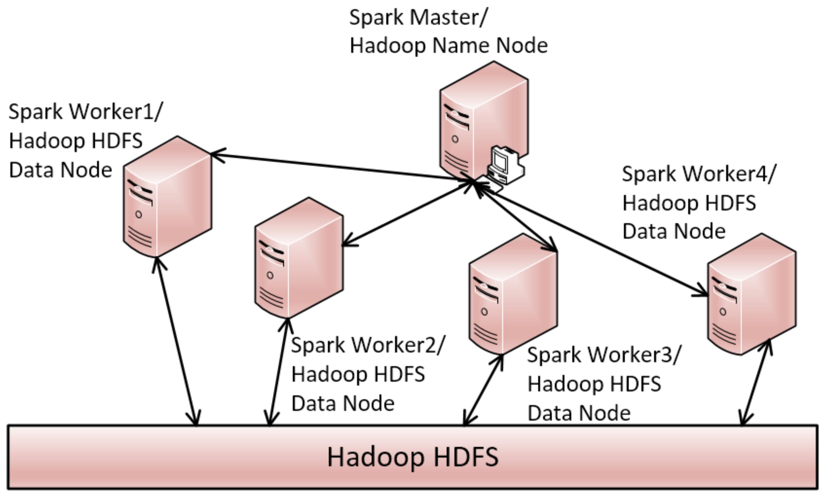
As mentioned above, a timeline query can be transformed into the computation of interval sets. When the timeline data become larger, the size of interval data will also increase rapidly. We intend to manage the big interval data on a Distributed Triangle Increment Tree, called DTI-Tree, to share the computation capacity between the machines on a Spark cluster shown in Figure 6. The DTI-Tree is an interval-based index supporting a data partition strategy named triangle increment tree method. It composes of two parts. Part one is a global index, called T-Tree, running on the master node. The master node is the computer on which the Spark master, the Hadoop Name Node and the driver programs execute. The global index is the external user interface that only managers some triangles. Part two is a lot of Triangle Increment Tree (TI-Tree) running on a slave node. A TI-Tree is a local index structure indexing all the interval points located in the triangle corresponding to one of the triangles in the global index. We employ the Hadoop Distributed File System (HDFS) to store the index data.
3.1. The Strategy of Partition
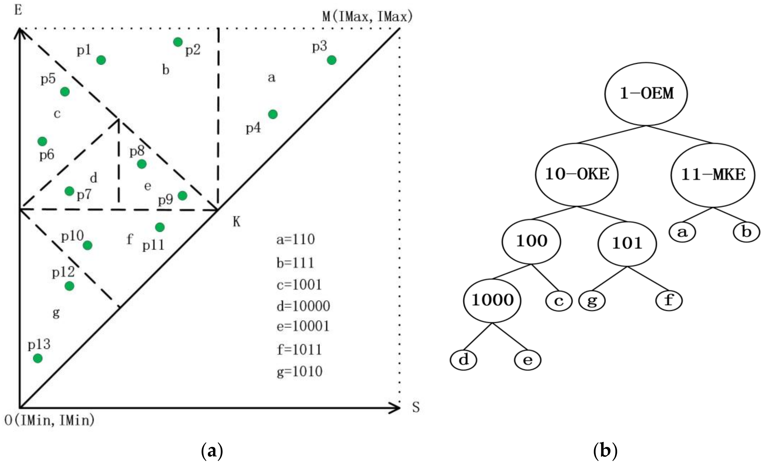
To manage interval data, we convert the interval object into a two-dimensional (2D) point in a 2D plane, as shown in Figure 4, and assume that all the interval points are in the basic triangle OEM shown in Figure 7a. The line OM is a segment in line NP shown in Figure 4. For the convenience of computing, we make OEM to be an isosceles right-angled triangle. To construct a binary tree indexing data objects, a recursive decomposition of the triangle is implemented. If the maximum number of interval points that a leaf triangle can contain is N = 2, then it is a recursive binary decomposition that all the leaf triangles will be decomposed recursively until each number of the interval points in a leaf triangle is less than N. Then, the decomposition will construct a binary tree shown in Figure 7b. This is the partition strategy that TD-Tree [8] used, we called it TD-tree’s partition strategy (TDPS).
The TDPS leads to a limitation that the range of interval dataset must be evaluated before index creation. That is, the minimum and maximum values of the original intervals should be known. It is easy for a small and static dataset, but not for a big or dynamic dataset. A tentative solution is to give a range that is as large as possible. However, it will result in another problem that the TD-Tree’s node identifier may overflow. Because the identifier is an integer that is represented by a binary string, the length of the binary string may be larger than 32 bits or 64 bits when the data set is very large. It is no longer easy to use an integer to represent a node’s identifier. All the benefits of using an integer as an identifier will disappear.
Hence, we design a partition strategy, called triangle increment partition strategy (TIPS), which is extended from TDPS. The only difference between TIPS and TDPS is that the root triangle area can be increased when the inserting interval point is out of the scope of the root triangle in the TIPS, while the TDPS cannot. That is, the TIPS compose of a triangle increment process and a decomposition process. The decomposition process is the same as the TDPS when the inserting interval points are in the root triangle.
Here, we only show that increment process. The process consists of a left extension procedure and a right extension. Assume that there is an isosceles right-angled triangle ABC called initial triangle or root triangle, and BC is always on the line NP (Figure 4). If there is an interval point located at the left of line AB, the left extension of ABC will be executed and results in a new isosceles right-angle root triangle GKC, as shown in Figure 8a. If there is a point located above the line AC, then the right extension of ABC will be carried out and it will result in a new isosceles right-angle root triangle DBE, as shown in Figure 8b. The TIPS is the basic ideas of the indexing method, TI-Tree, used as local index on slave node presented in this paper. The TIPS algorithm shown in Algorithm 1.
| Algorithm 1: Tips |
| Input: pi: an interval [Is, Ie]; root: root node of TI-Tree or T-Tree; Output: root: the new root node { 1. read the root node from disk; 2. if (root._triangle contains pi) return root; 3. if (pi is located at the left of line AB) executes left extension shown in Figure 8a; else executes right extension shown in Figure 8b; 4. while (root. _triangle does not contain pi) call Algorithm 1 recursively; 5. return root; } |
4. The Structure of DTI-Tree
The intervals of a timeline are stored on a TI-Tree. They consist of some objects [Tid, Iid, Is, Ie, It], where [Is, Ie] is the spatial location on a 2D plane (Figure 7a), defined by the start value and the end value of the data. Each object belongs to a triangle partition, as shown in Figure 7a. The DTI-Tree is a combination of T-Tree and TI-Trees that are processed by each slave node in the cluster. Let M be the master node and have n slave nodes. Each slave node is recorded as Si and i [0, n − 1]. Each slave node has one or K TI-Trees. They may be recorded as
Therefore,
For example, if the data in triangle OEM (Figure 7a) are stored in two slaves, then the dataset will be partitioned into two parts, triangle OKE and EKM. One T-Tree will be constructed in the master node, and Tow TI-Trees, TI-Tree1 (OKE) and TI-Tree2 (EKM) will be constructed in slave 1 and slave 2, as shown in Figure 9. Because the` TI-Tree is a virtual binary tree without non-leaf nodes, all of the leaf nodes with codes (The triangle codes are in Figure 7a) in a TI-Trees form a linear leaf node list. Each triangle contains one or more interval points, which are parts of a timeline storing in HDFS. DTI-Tree has five layers: master, slave, leaves, intervals, and timelines, as shown in Figure 9. A timeline is possible to be partitioned to two or more slaves, for example, the timeline T1 in the Figure 9 has two partitions, one is in the slave1, and the other is in the slave 2. The following are the construction, maintenance, and query of DTI-Tree.
4.1. The Construction of DTI-Tree
The DTI-Tree construction is carried out by the Spark cluster. The DTI-Tree could be built in three phases: data partition, T-Tree construction and TI-Trees construction. The first phase is collaboratively executed in parallel in the Spark cluster, and the other two phases are separately executed on the slaves.
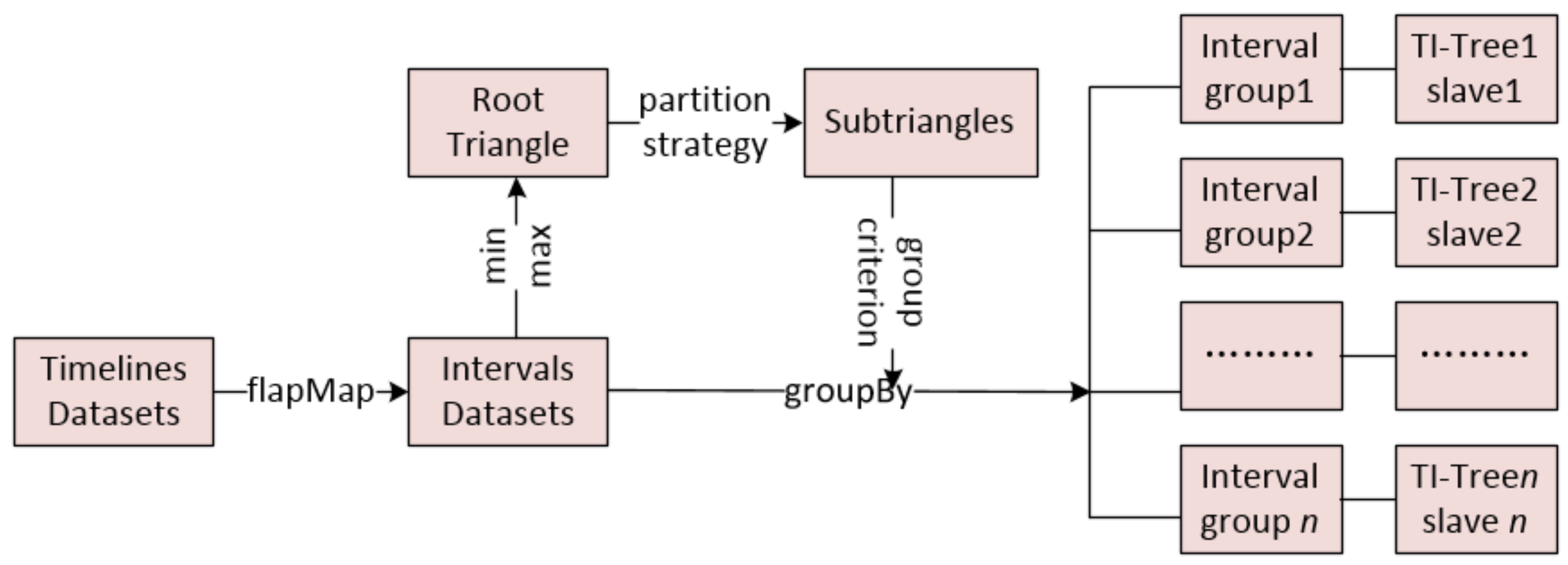
According to Equation (4), a DTI-Tree has a global index, T-Tree, in the master node, and a series of TI-Trees in n slave nodes. Assume that TD is a timeline data set, the total number of timeline objects is TN, Tt is a timeline in TD and t [0, TN − 1]. The first step of the data partition is to load the timeline data set from HDFS and to call the function flapMap in Table 3 to execute a mapping from timeline data set to interval data set IDS. Then, we get the minimum and maximum values of the interval data set IDS from the interval Spark Resilient Distributed Datasets (RDD) by calling the functions max and min in Table 3. A root triangle of the T-Tree will be set up on the base of the minimum value and maximum value by the algorithm that is presented in [9]. The root triangle will be partitioned into n sub triangles by the partition strategy that is mentioned in Section 3.1. Each sub triangle is related to a slave node. The last step is to call the function groupBy listed in Table 3 to form n groups according to the interval point location in a certain sub triangle. The main construction process is shown in Figure 10. The second phase is the construction of T-Tree according to the sub triangles. Its construction is simple because the T-Tree is an absolute binary search tree. The last phase is the constructions of TI-Trees. The TI-Tree is an extension of the TD-Tree’s [8]. They share almost all the algorithms except the construction methods. The Algorithm 2 shows the process for constructing TI-Trees.
| Algorithm 2: TI-Tree construction |
| Input: IDS: an interval data set; Output: TI-Tree { 1. initial the root triangle variable root; 2. i = 0; 3. while (i < IDS.size()) if (root._triangle.constains(IDS [i])) call the TD-Tree’s insertion procedure; i++; else call Algorithm 1; 4. return TI-Tree. } |
The partition strategy that is used by the construction may result in skewing due to the unbalanced distribution of the interval points. A distributed index has a good balance when the standard deviation ≤ 1% [35]. The Equations (5) and (6) calculate the standard deviation by calling the function count to return the number of interval points in slave Si. If the standard deviation is larger than the threshold given, the slave that has the maximum value of should be partitioned into two parts, reconstruct two TI-Trees in the same slave node, and inform the T-Tree in the master node to adjust tree. The Algorithm 3 shows the construction method of the DTI-Tree.
| Algorithm 3: DTI-Tree construction shown in Figure 10 |
| Input: TD: a timeline data set; Output: DTI-Tree { 1. IDS= flapMap(TD); //convert timeline set into interval set. 2. initialize and recursively binary split the root triangle by TIPS until the number of the leaf node triangle is equal to the number of all the slaves SN in the cluster; 3. call the function groupBy to split IDS into SN groups according to the leaf nodes’ triangles generated in Step 2; 4. executes load balance evaluation and avoid adjustment after construction; 5. for each group, call Algorithm 2 to construct TI-Tree on the corresponding slave; } |
4.2. The Update of DTI-Tree
After the construction of DTI-Tree, a new timeline may be inserted into the index and an existing timeline may be deleted from the index. To insert a new timeline, we select the minimum triangle that contains all the interval points of the timeline. If the minimum triangle is a slave root triangle, let the corresponding TI-Tree insert all the interval points of the timeline. If the minimum triangle contains several slave root triangles, divide the timeline and let the corresponding TI-Trees insert the partitioned interval points, respectively. The Algorithm 4 summaries the process of the insertion method.
| Algorithm 4: DTI-Tree insertion |
| Input: T: a timeline; Output: DTI-Tree { 1. call the function intervalize listed in Table 3 to get a set of interval points IPS; 2. select the minimum triangle minTri which contains IPS; 3. get the slaves whose root triangle is intersected with minTri; 4. if (the number of slaves is equal 1) let the corresponding TI-Tree insert all the interval points of the timeline else divide the IPS into several parts; let the corresponding TI-Tree insert each part. } |
4.3. The Timeline Similarity Query of DTI-Tree
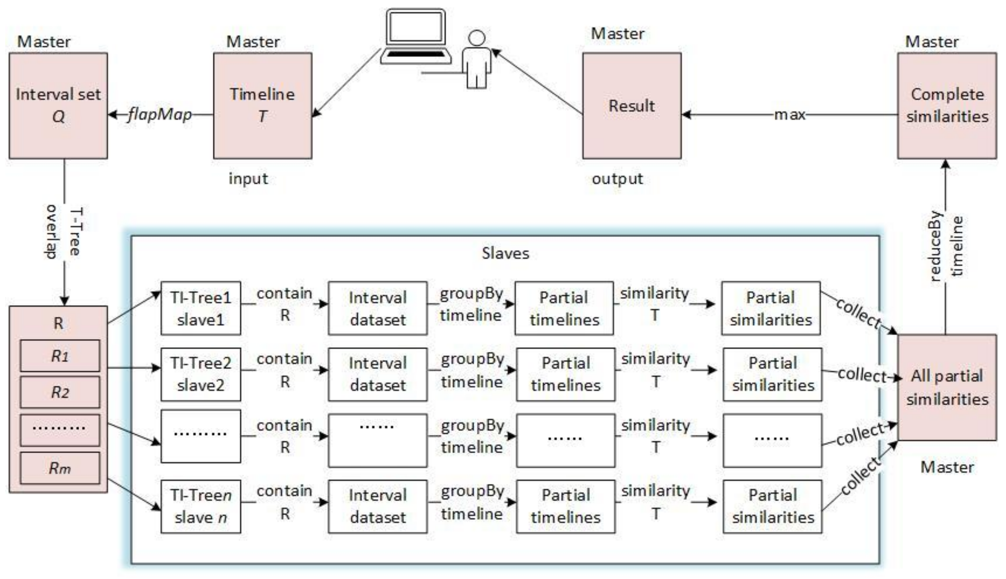
In this section, we discuss the query algorithm of timeline similarity as an example. The similarity between two timelines are defined in Equation (1). All the operations of DTI-Tree depend on interval set operations. Hence, the first step is to convert the timeline T into an interval set Q using the function intervalize that is listed in Table 3. Then, the overlaps query region of each interval in Q is calculated by the method that is presented in the reference [9]. Theoretically, we should make a query for each rectangle. But, this results in a lot of repetitive computations and network IO times. Consequently, we combine the resulting rectangles into a rectangle R. Although it broadens the range of the query in some degree, it can significantly reduce network IO times. The next step is to find all of the slave root triangles overlapping with R. Let the TI-Tree in each corresponding slave run overlap query [9] and return all of the interval points in the rectangle R. Group these interval points by the timeline ID and form some local partial timelines. Calculate the partial similarity between each local partial timeline and the timeline T and return the results to the master. All of the partial similarity values received by the master are grouped by the timeline ID, and the similarity of each complete timeline and T is obtained using the function reduce that listed in Table 3. At last, the timeline ID with the maximum similarity value will be returned. The Algorithm 5 summaries the process of the similarity query method and Figure 11 shows the main steps.
| Algorithm 5: DTI-Tree similarity query shown in Figure 11 |
| Input: T: a timeline; Output: the most similar timeline to T { 1. call the function intervalize to get a set of interval points Q = {Q0, Q1, …, Qk, …, Qm}; 2. calculate the overlap query region of Qk, noted as Rk; R = R0 R1, …, Rk, …, Rm; 3. find all the slave root triangles which overlaps R by the T-Tree in the master node, the result is {RTi}. RTi is the root triangle of the TI-Treei on the slave node Si. 4. find all the interval points Pi in the rectangle R by the TI-Treei on the slave Si separately; 5. execute Pi .groupBy(timeline ID) on the slave Si separately, and the result is some partial timelines PTi={PTij}; 6. execute similarity (T, PTij) and send the result that are some partial similarity values PSVi to the master; 7. combine all the partial similarity values {PSVij} on the master node, here i is a slave identifier and j is a timeline identifier; 8. return the result of {PSVij}. reduceBy(j). max (); } |
5. Experimental Evaluation
In order to verify the algorithm proposed in this paper, we performed an experimental evaluation of the DTI-Tree. DTI-Tree is an indexing method for interval-based discrete timelines similarity query based on Apache Spark. We performed an experimental evaluation of the DTI-Tree and compared it to the R-Tree in GeoSpark [33]. The R-Tree in GeoSpark was chosen because it provides the same properties as our approach that can index discrete interval data collections based on Spark. In addition, the family of R-Trees is still the most popular index structure that is used for general spatio-temporal data and is provided by platforms, such as Hadoop, MongoDB, Oracle, MySQL, PostgreSQL, Microsoft SQL Server, and more. An interval object will be treated as a two-dimensional point in R-Tree in our experimental evaluation. Furthermore, a timeline generator and two benchmark datasets will be presented in this experiment.
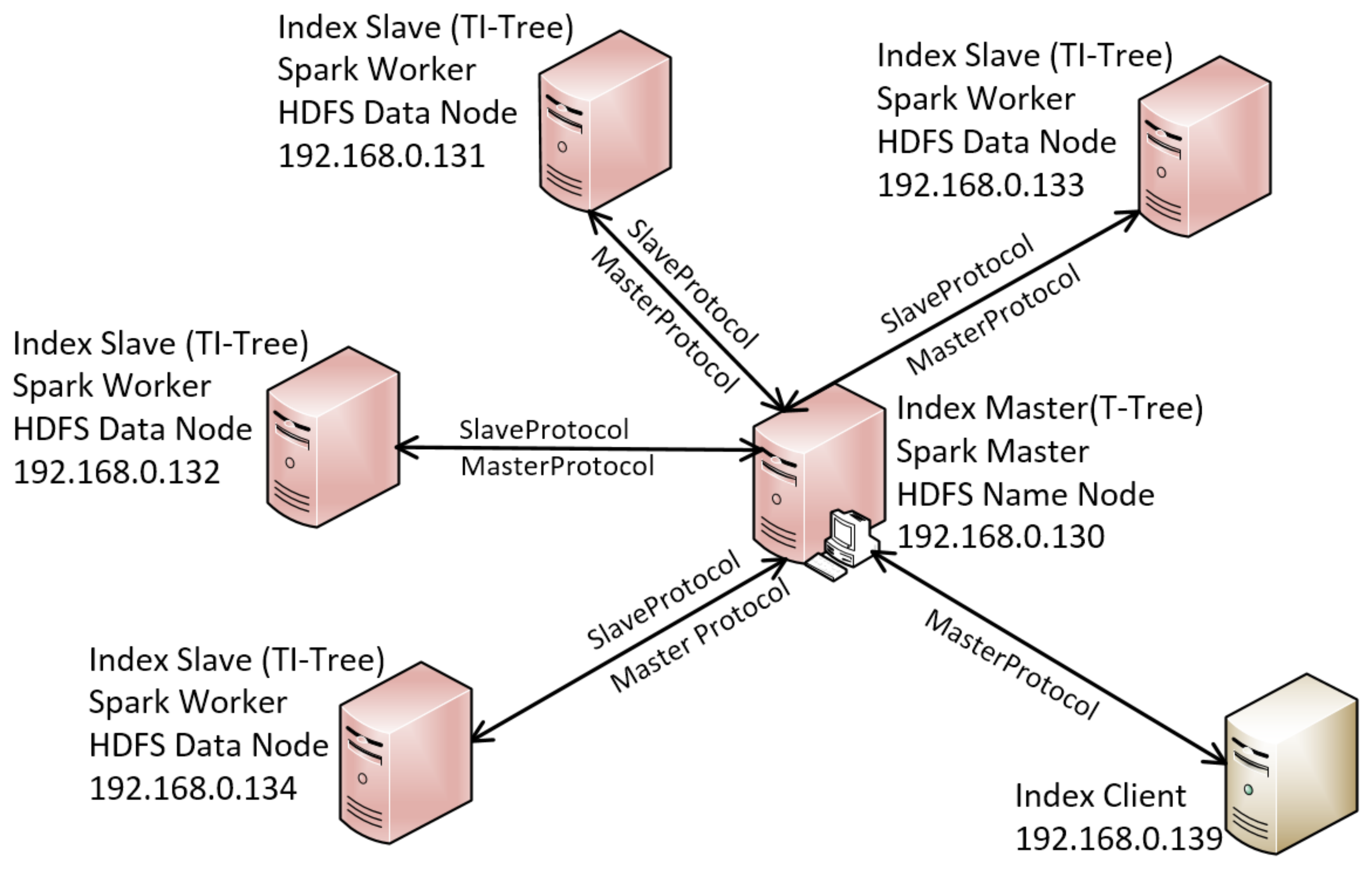
As mentioned in the previous sections, the timeline data are stored in HDFS. We use Spark (version 2.2.1) RDD to load the dataset from HDFS (version 2.7.3). Without special instructions, all of the experimental results were computed on a cluster, including five computers, as shown in Figure 12. The HDFS name node, Spark master and index master are on the same node which is a workstation computer with the configuration of two 2.80 GHZ Intel(R) Xeon(R) CPUs, and 32 GB RAM. Each slave node is a computer which has 16 GB RAM, a 64-bit dual core i5 processor, and a 7200 rpm 1TB disk. It plays roles of the HDFS data node, Spark worker, and index slave. The client is a computer that has an Intel® Core™ i7 processor and 8 GB RAM. The communications among the master node, the slave node, and the client are implemented by the Hadoop Remote Procedure Call (RPC) (https://wiki.apache.org/hadoop/HadoopRpc). We design two protocol interfaces, called MasterProtocol and SlaveProtocol, to support the communications. The operation systems of the cluster are all Ubuntu 16.04. All the algorithms are implemented by java (JDK 1.8.0_144) using IntelliJ IDEA 2017 (community edition).
To test the performance of the index method, we develop a timeline data generator, called TimelineGenerator (https://github.com/ZhenwenHe/gtl_for_java/tree/master/src/main/java/gtl/index/itree/TimelineGenerator), for generating the simulated random dataset, which fits for some special requirements. The random number generator used in TimelineGenerator is the UniformGenerator of Spark MLlib (https://spark.apache.org/mllib/). The TimelineGenerator belongs to the open source project gtl_for_java (https://github.com/ZhenwenHe/gtl_for_java.git) on GitHub. The TimelineGenerator generates various timeline test datasets by controlling the parameters that are listed in Table 4. The first experimental dataset, named DS1, was generated by the TimelineGenerator with the default parameters. It has 10,000,000 timelines and about 55.6 million intervals. The dataset DS1 is about 0.7 TB and represents short timelines. The second experimental dataset, named DS2, was generated by the TimelineGenerator, with the parameters timelineMinLength = 50, timelineMaxLength = 100, and intervalAttachment = [5k,10k]. The dataset DS2 also has 10,000,000 timelines, but it has about 1.3 billion intervals. It is about 1.6 TB and represents the long timelines.
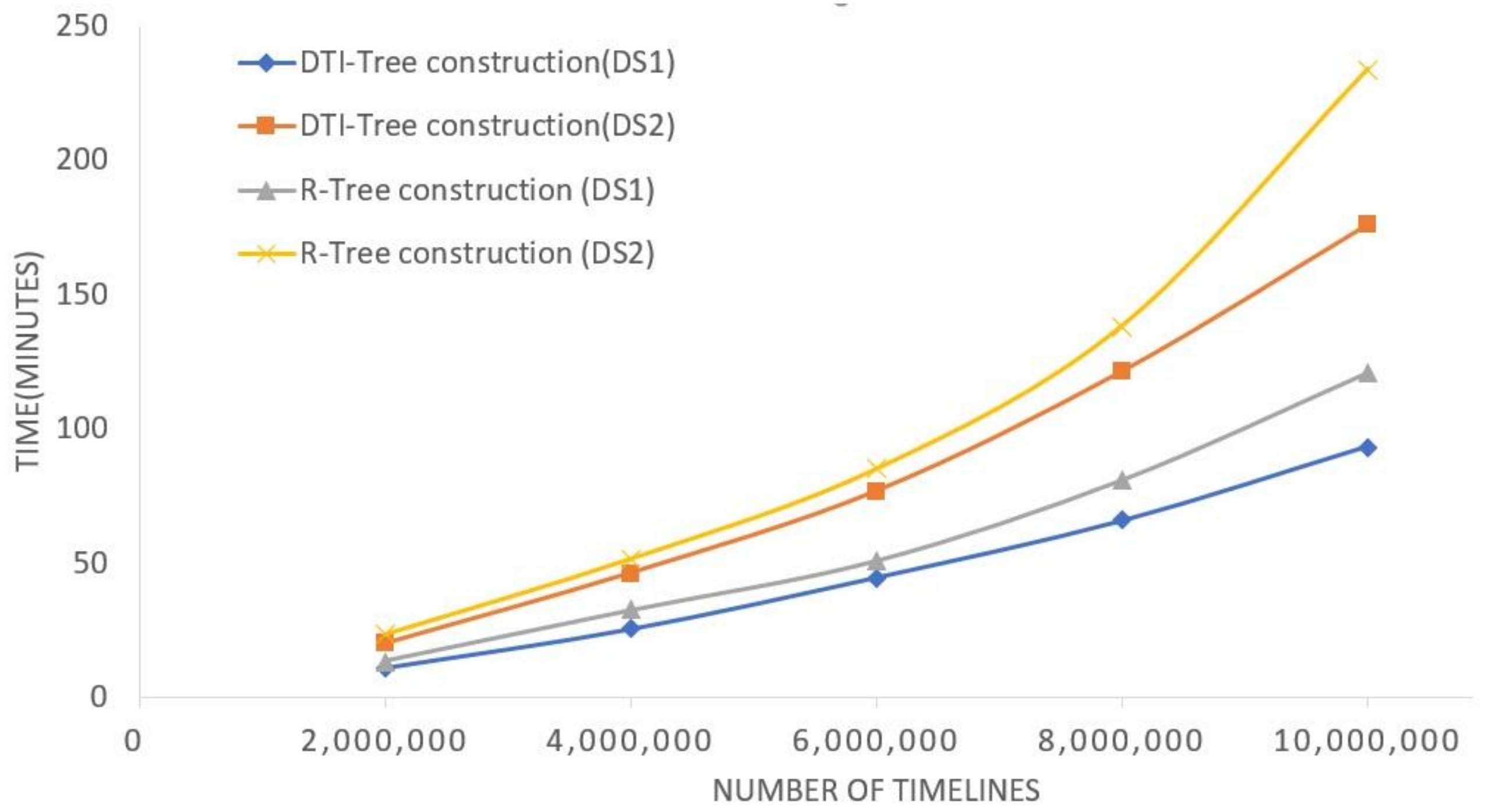
The experimental results of index construction performance test are shown in Figure 13. The X axis is the number of timeline objects involved in the experiment. The Y axis is the time cost. The DTI-Tree and R-Tree were constructed with the number of timeline objects varying from 1,000,000 to 10,000,000. There are eight fixed partitions for running this test. The result shows that the DTI-Tree has higher construction performance than the R-Tree. The result also shows that the DTI-Tree has lower performance when it handles the long timeline dataset DS2. The reason is that the longer the average length of the intervals, the bigger the dataset, and the computation takes a longer time to construct the DTI-Tree. Therefore, it is better to implement the DTI-Tree construction by bulk loading of the dataset to reduce the Spark RDD construction time cost.
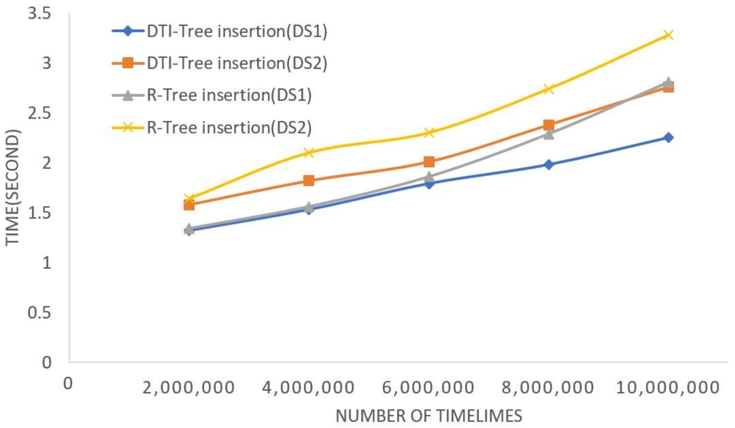
The experimental results of insertion performance comparison by varying number of timelines are shown in Figure 14. The X axis represents time cost, it is the average time for 100 times operations. The number of timelines varies from 1,000,000 to 10,000,000. The result shows that the DTI-Tree has higher performance than R-tree. In addition, the average length of the timelines affects the insertion performance. Because the TI-Tree manages all of the interval datasets, the leaf node map and empty leaf node list of the TI-Tree have a bigger size, while the Number of intervals increases. The insertion operations on the map and list will take more time. Another we can observe from the results is that the average time cost of deletion is slightly smaller than the insertion’s. It is because that the empty leaf node list may be scanned when a new leaf node appears, and the empty leaf node list will involve every splitting in the process of insertion. However, there are not these operations in the process of deletion. There is only one case that the empty leaf node list will be add an element when the leaf node only contains one interval object, which will be deleted from the leaf node.
Figure 15 shows the relationship between the average time cost of similarity query and the total number of timeline objects that are involved in each query. The number of timelines varies from 1,000,000 to 10,000,000 in DS1 and DS2. The DTI-Tree has better performance when it is indexing the short timelines dataset DS1. The main time cost of similarity query is to receive the intervals that are related to the query timeline. The major influenced factor is the leaf node map size in each TI-Tree. The more the intervals are, the bigger the leaf node map size is. The test result proves this deduction.
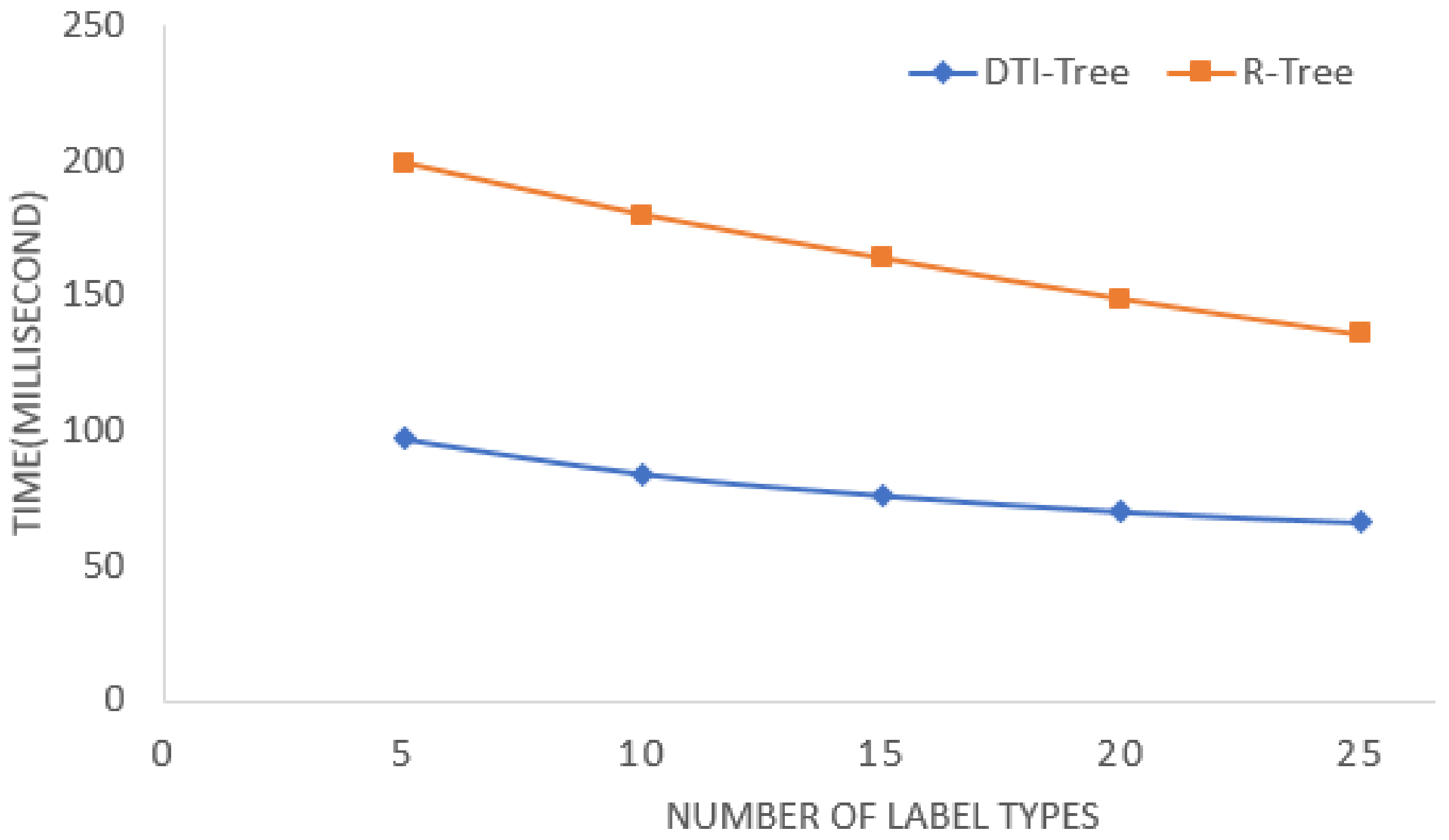
To test the impact of the label types in the process of similarity query, we change the label types in DS1 from 5 to 25. If the query input timeline is same as Figure 15, that is the query input timeline’s label types is fixed, the results of DTI-Tree and R-Tree are shown in Figure 16. The similarity query performance will slightly improve, because the RDD filter function can filtrate more intervals by label type equation to reduce the similarity computation in the later stage. However, if the label types of the input timeline for query increase with the DS1’s label types, then the similarity query performance will not change or decrease slightly. In the other words, the impact of the label types is slight because the impact is mainly in memory computation. When comparing to the disk IO and network IO, the memory computation time is a little part of them.
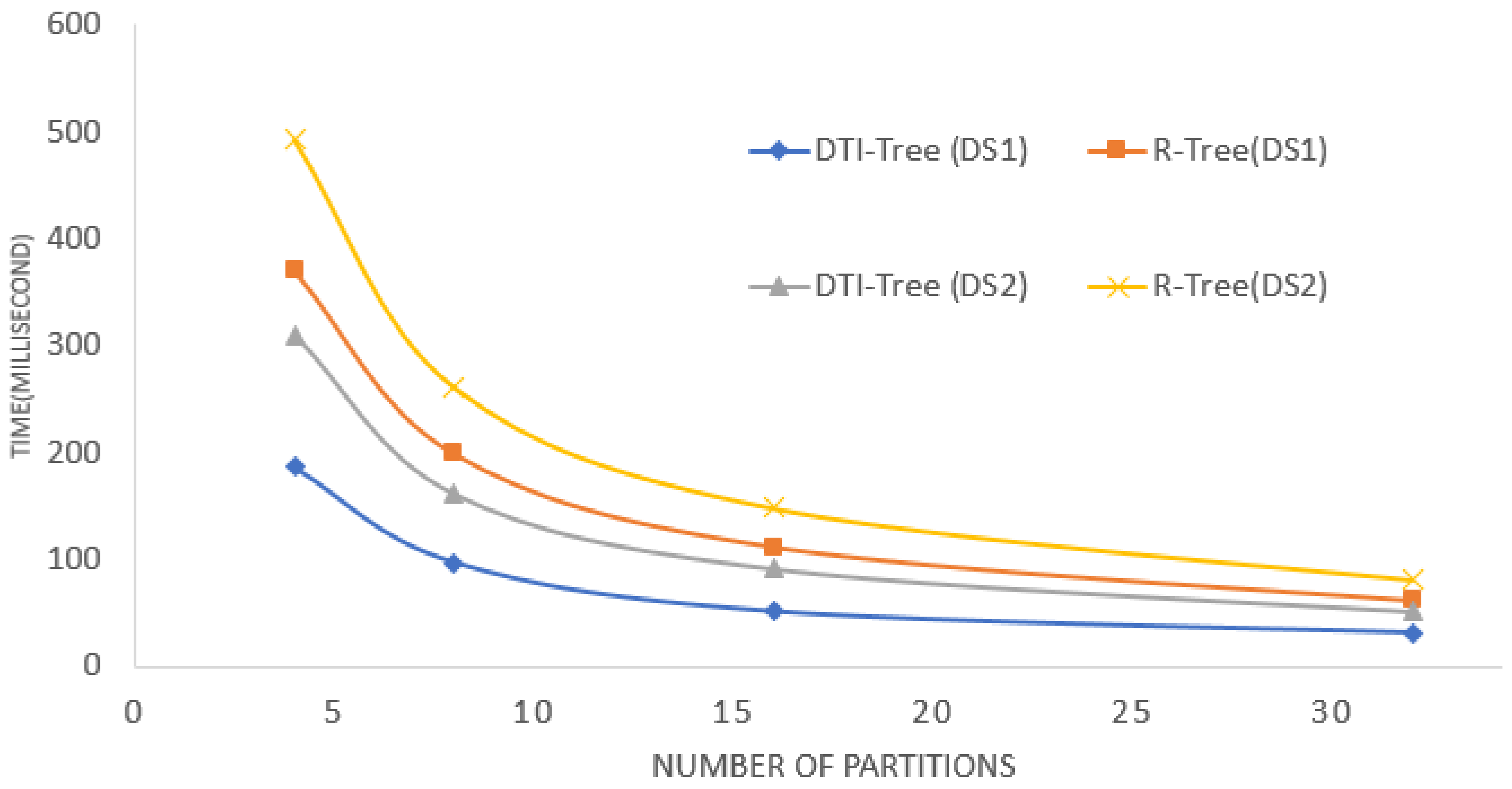
To test the influence of the partitions in the process of similarity query, we change the partitions from 4 to 32. The result is shown in Figure 17. It shows that the similarity query performance will increase with the increment of the partitions. Whether the dataset is DS1 or DS2, the conclusion is right. However, the communication costs among the slaves increase as the number of slaves increases. It results in the slower performance growth as the slaves increase, as shown in Figure 17.
In summary, the experimental results shown in the figures from Figure 13, Figure 14, Figure 15, Figure 16 and Figure 17 present that our proposed index structure, DTI-Tree, can efficiently process timeline similarity queries in distributed platforms and has higher performance than R-Tree in GeoSpark. The more partitions may improve the index performances and the index has scalability.
6. Conclusions
We investigated a novel problem of organizing and processing timelines in this paper. A distributed access approach name DTI-Tree for indexing timelines was presented. This index convers timelines into labeled intervals. The TIPS was proposed to support the representation and partition of the interval dataset for indexing timeline datasets. It fixes the deficiency of TDPS that is used in the TD-Tree and TB-Tree. The DTI-Tree are designed and implemented based on the TIPS. It consists of one T-Tree and one or more TI-Trees. The T-Tree is a virtual binary tree for indexing triangles. The TI-Trees are designed for indexing labeled intervals. All the root triangles of the TI-Trees are managed by the T-Tree. The T-Tree is running in the master node, while the TI-Trees are running in slave nodes. The communications between master and slave nodes are implemented by MasterProtocol and SlaveProtocol RPC interfaces. We employ the Apache Spark RDD to implement the DTI-Tree to achieve framework scalability. The timeline similarity formula was proposed in this paper, and the timeline similarity query was implemented based on the DTI-Tree. The experimental results show that the DTI-tree provides an effective distributed index solution to big timeline data and it has higher performance than Geopark’s R-Tree.
In addition, we developed an open source timeline test dataset generator, named TimelineGenerator. It can generate various timeline test datasets for different conditions and may provide some benchmark timeline datasets for the future research. In the next study, we plan to use another distributed computing framework to replace the Spark RDD, and to handle bigger size timeline dataset on the Tianhe-2, which is one of the Top 2 supercomputers in the world.
Acknowledgments
The work described in this paper was supported by the National Natural Science Foundation of China (41572314, U1711267, 41101368).
Author Contributions
The manuscript was written by Zhenwen He. Xiaogang Ma revised the manuscript and participated in designing the experiments. All authors reviewed the manuscript.
Conflicts of Interest
The authors declare no conflicts of interest.
References
- Brehmer, M.; Lee, B.; Bach, B.; Riche, N.H.; Munzner, T. Timelines revisited: A design space and considerations for expressive storytelling. IEEE Trans. Vis. Comput. Graph. 2017, 23, 2151–2164. [Google Scholar] [CrossRef] [PubMed]
- Camerra, A.; Palpanas, T.; Shieh, J.; Keogh, E. Isax 2.0: Indexing and Mining One Billion Time Series. In Proceedings of the 2010 10th IEEE International Conference on Data Mining (ICDM), Sydney, NSW, Australia, 14–17 December 2010; Institute of Electrical and Electronics Engineers Inc.: Sydney, NSW, Australia, 2010; pp. 58–67. [Google Scholar]
- Zoumpatianos, K.; Idreos, S.; Palpanas, T. Ads: The adaptive data series index. VLDB J. 2016, 25, 843–866. [Google Scholar] [CrossRef]
- Yagoubi, D.E.; Akbarinia, R.; Masseglia, F.; Palpanas, T. Dpisax: Massively distributed partitioned isax. In Proceedings of the 2017 17th IEEE International Conference on Data Mining (ICDM), New Orleans, LA, USA, 18–21 November 2017; IEEE Computer Society Press: New Orleans, LA, USA, 2017; pp. 1135–1140. [Google Scholar]
- Kondylakis, H.; Dayan, N.; Zoumpatianos, K.; Palpanas, T. Coconut: A scalable bottom-up approach for building data series indexes. Proc. VLDB Endow. 2018, 11, 677–690. [Google Scholar]
- Kriegel, H.P.; Potke, M.; Seidl, T. Interval sequences: An object-relational approach to manage spatial data. In Proceedings of the 2001 7th International Symposium Advances in Spatial and Temporal Databases (SSTD), Redondo Beach, CA, USA, 12–15 July 2001; Jensen, C.S., Schneider, M., Seeger, B., Tsotras, V., Eds.; Springer: Berlin, Germany, 2001; Volume 2121, pp. 481–501. [Google Scholar]
- Kriegel, H.-P.; Pötke, M.; Seidl, T.; Jensen, C.; Schneider, M.; Seeger, B.; Tsotras, V. Object-relational indexing for general interval relationships. In Advances in Spatial and Temporal Databases; Springer: Berlin/Heidelberg, Germany, 2001; Volume 2121, pp. 522–542. [Google Scholar]
- Stantic, B.; Topor, R.; Terry, J.; Sattar, A. Advanced indexing technique for temporal data. Comput. Sci. Inf. Syst. 2010, 7, 679–703. [Google Scholar] [CrossRef]
- He, Z.; Kraak, M.-J.; Huisman, O.; Ma, X.; Xiao, J. Parallel indexing technique for spatio-temporal data. ISPRS J. Photogramm. Remote Sens. 2013, 78, 116–128. [Google Scholar] [CrossRef]
- Ma, X.; Fox, P. Recent progress on geologic time ontologies and considerations for future works. Earth Sci. Inform. 2013, 6, 31–46. [Google Scholar] [CrossRef]
- Ma, X.; Carranza, E.J.M.; Wu, C.; van der Meer, F.D.; Liu, G. A skos-based multilingual thesaurus of geological time scale for interoperability of online geological maps. Comput. Geosci. 2011, 37, 1602–1615. [Google Scholar] [CrossRef]
- He, Z.; Wu, C.; Liu, G.; Zheng, Z.; Tian, Y. Decomposition tree: A spatio-temporal indexing method for movement big data. Clust. Comput. 2015, 18, 1481–1492. [Google Scholar] [CrossRef]
- Xie, X.; Mei, B.; Chen, J.; Du, X.; Jensen, C.S. Elite: An elastic infrastructure for big spatiotemporal trajectories. VLDB J. 2016, 25, 473–493. [Google Scholar] [CrossRef]
- Elmasri, R.; Wuu, G.; Kim, Y. The Time Index: An Access Structure for Temporal Data. In Proceedings of the 16th International Conference on Very Large Databases, Brisbane, Australia, 13–16 August 1990; pp. 1–12. [Google Scholar]
- Curtis, P.K.; Michael, S. Segment Indexes: Dynamic Indexing Techniques for Multi-Dimensional Interval Data. SIGMOD Rec. 1991, 20, 138–147. [Google Scholar]
- Chaabouni, M.; Chung, S.M. The point-range tree: A Data Structure for Indexing Intervals. In Proceedings of the 1993 ACM Conference on Computer Science, Washington, DC, USA, 25–28 May 1993; ACM: Indianapolis, IN, USA, 1993; pp. 453–460. [Google Scholar]
- Ang, C.H.; Tan, K.P. The interval B-tree. Inf. Process. Lett. 1995, 53, 85–89. [Google Scholar] [CrossRef]
- Tsotras, V.J.; Gopinath, B.; Hart, G.W. Efficient management of time-evolving databases. IEEE Trans. Knowl. Data Eng. 1995, 7, 591–608. [Google Scholar] [CrossRef]
- Lanka, S.; Mays, E. Fully Persistent B+-Trees. SIGMOD Rec. 1991, 20, 426–435. [Google Scholar] [CrossRef]
- Brodal, G.S.; Brodal, L.; Tsakalidis, K.; Sioutas, S.; Tsichlas, K. Fully Persistent B-Trees. In Proceedings of the 23rd annual ACM-SIAM Symposium on Discrete algorithms, Kyoto, Japan, 17–19 January 2012; Society for Industrial and Applied Mathematics: Kyoto, Japan, 2012; pp. 602–614. [Google Scholar]
- Kriegel, H.-P.; Pötke, M.; Seidl, T. Managing intervals efficiently in object-relational databases. In Proceedings of the 26th International Conference on Very Large Data Bases, San Francisco, CA, USA, 10–14 September 2000; Morgan Kaufmann Publishers Inc.: San Francisco, CA, USA, 2000; pp. 407–418. [Google Scholar]
- Enderle, J.; Schneider, N.; Seidl, T. Efficiently processing queries on interval-and-value tuples in relational databases. In Proceedings of the 31st International Conference on Very Large Data Bases, Trondheim, Norway, 30 August–2 September 2005; VLDB Endowment: Trondheim, Norway, 2005; pp. 385–396. [Google Scholar]
- Wang, M.; Xiao, M. SHB+-tree: A segmentation hybrid index structure for temporal data. In Proceedings of the 2015 15th International Conference on Algorithms and Architectures for Parallel (ICA3PP), Zhangjiajie, China, 18–20 November 2015; Wang, G., Zomaya, A., Martinez Perez, G., Li, K., Eds.; Springer International Publishing: Cham, Switzerland, 2015; pp. 282–296. [Google Scholar]
- Bayer, R.; McCreight, E.M. Organization and maintenance of large ordered indexes. Acta Inform. 1972, 1, 173–189. [Google Scholar] [CrossRef]
- Douglas, C. Ubiquitous B-tree. ACM Comput. Surv. (CSUR) 1979, 11, 121–137. [Google Scholar]
- Guttman, A. R-trees: A dynamic index structure for spatial searching. SIGMOD Rec. 1984, 14, 47–57. [Google Scholar] [CrossRef]
- Kim, J.; Nam, B. Parallel multi-dimensional range query processing with R-trees on GPU. J. Parallel Distrib. Comput. 2013, 73, 1195–1207. [Google Scholar] [CrossRef]
- Eldawy, A.; Mokbel, M.F. Spatialhadoop: A mapreduce framework for spatial data. In Proceedings of the 2015 31st IEEE International Conference on Data Engineering, Seoul, Korea, 13–17 April 2015; IEEE Computer Society: Seoul, Korea, 2015; pp. 1352–1363. [Google Scholar]
- Dean, J.; Ghemawat, S. Mapreduce: Simplified data processing on large clusters. Commun. ACM 2008, 51, 107–113. [Google Scholar] [CrossRef]
- Aji, A.; Wang, F.; Vo, H.; Lee, H.; Liu, Q.; Zhang, X.; Saltz, J. Hadoop gis: A high performance spatial data warehousing system over mapreduce. Proc. VLDB Endow. 2013, 6, 1009–1020. [Google Scholar] [CrossRef]
- Alarabi, L.; Mokbel, M.F.; Musleh, M. St-hadoop: A mapreduce framework for spatio-temporal data. In Proceedings of the 2017 15th International Symposium Advances in Spatial and Temporal Databases (SSTD), Arlington, VA, USA, 21–23 August 2017; Gertz, M., Renz, M., Zhou, X., Hoel, E., Ku, W.-S., Voisard, A., Zhang, C., Chen, H., Tang, L., Huang, Y., et al., Eds.; Springer International Publishing: Cham, Switzerland, 2017; pp. 84–104. [Google Scholar]
- Yu, J.; Wu, J.X.; Sarwat, M. Geospark: A Cluster Computing Framework for Processing Large-Scale Spatial Data; Assoc Computing Machinery: New York, NY, USA, 2015. [Google Scholar]
- Baig, F.; Mehrotra, M.; Vo, H.; Wang, F.; Saltz, J.; Kurc, T. Sparkgis: Efficient comparison and evaluation of algorithm results in tissue image analysis studies. In Proceedings of the Biomedical Data Management and Graph Online Querying: VLDB 2015 Workshops, Big-O(Q) and DMAH, Waikoloa, HI, USA, 31 August–4 September 2015; Wang, F., Luo, G., Weng, C., Khan, A., Mitra, P., Yu, C., Eds.; Revised Selected Papers. Springer International Publishing: Cham, Switzerland, 2016; pp. 134–146. [Google Scholar]
- Wang, H.; Belhassena, A. Parallel trajectory search based on distributed index. Inf. Sci. 2017, 388–389, 62–83. [Google Scholar] [CrossRef]
- Jalili, V.; Matteucci, M.; Masseroli, M.; Ceri, S. Indexing next-generation sequencing data. Inf. Sci. 2017, 384, 90–109. [Google Scholar] [CrossRef]
Figure 1.
The difference between a timeline and a time series.

Figure 2.
Some Empires of China, Japan, and Korea (https://timelinestoryteller.com/#examples).
Figure 2.
Some Empires of China, Japan, and Korea (https://timelinestoryteller.com/#examples).
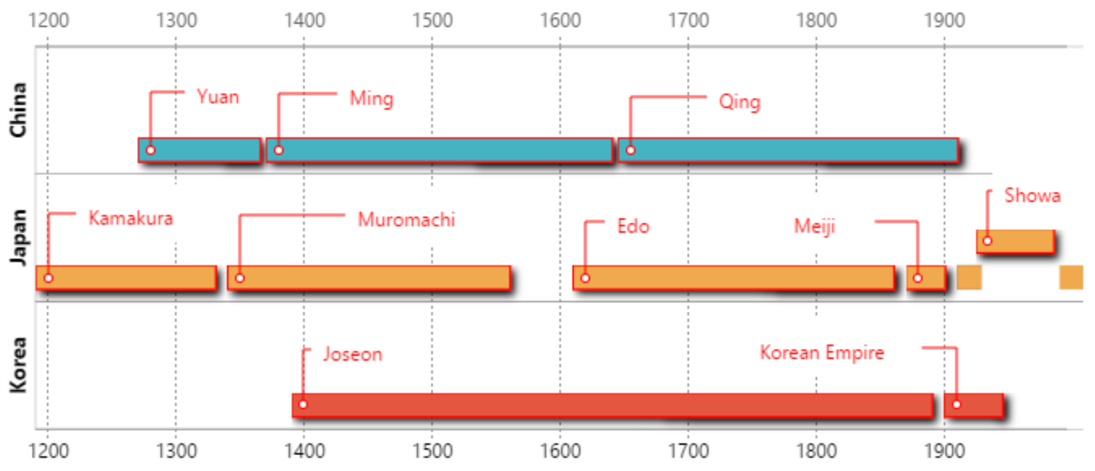
Figure 3.
Daily timelines of worker, researcher, and pupil.
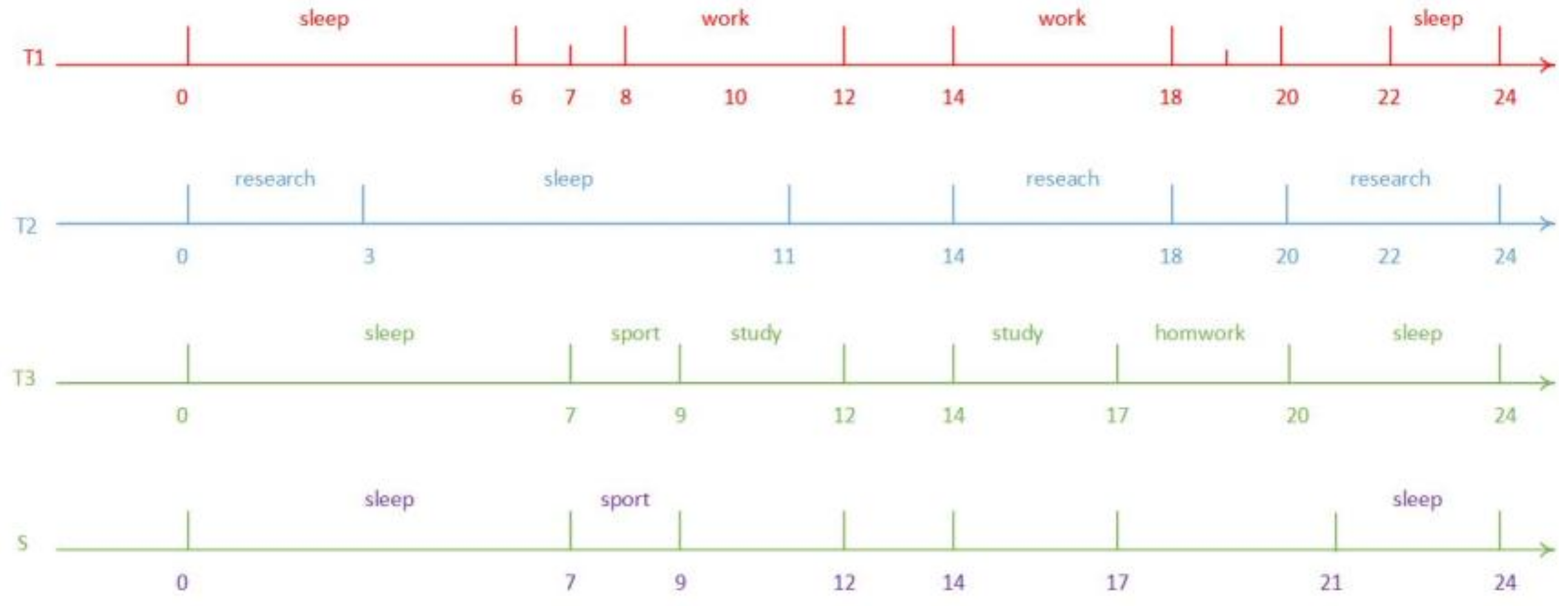
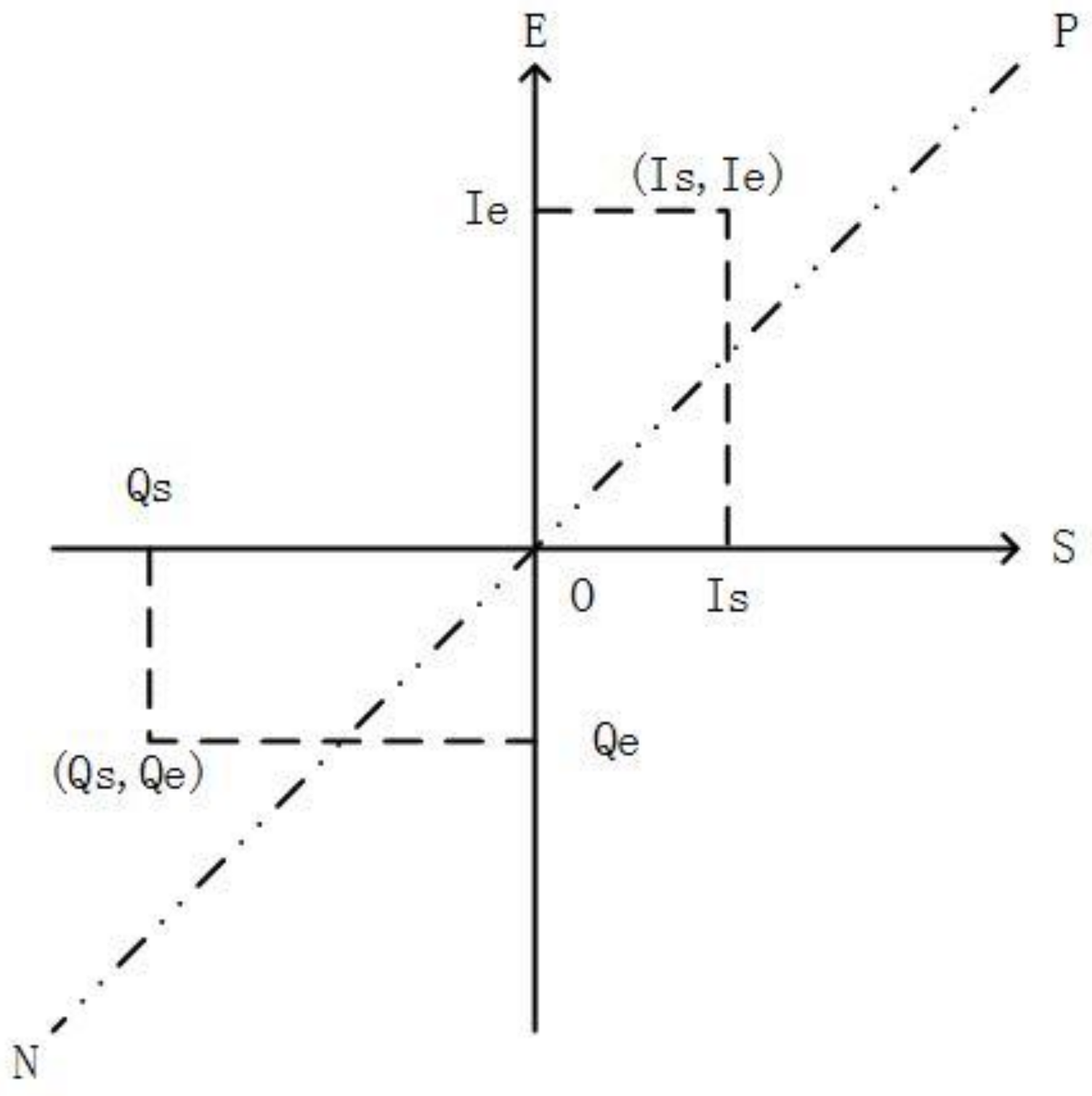
Figure 5.
An example of two timelines similarity computation process.
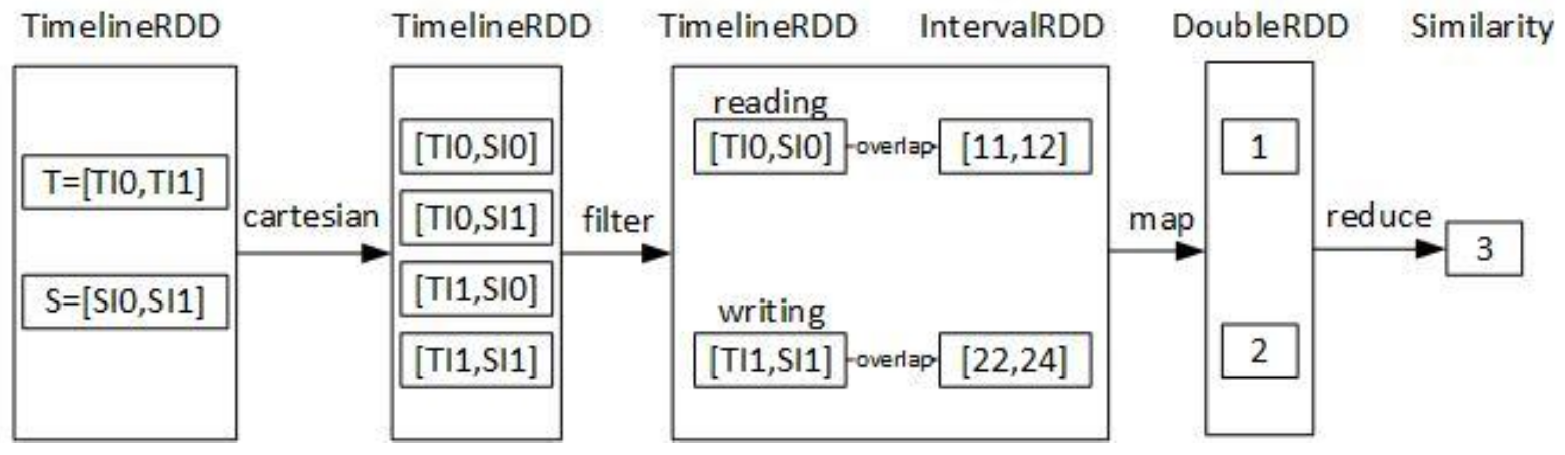
Figure 6.
Distributed Triangle Increment Tree (DTI-Tree) system architecture.

Figure 7.
TD-tree’s partition strategy (TDPS) and triangle binary tree. (a) TD-Tree’s triangle decomposition; (b) Triangle binary tree with codes.
Figure 7.
TD-tree’s partition strategy (TDPS) and triangle binary tree. (a) TD-Tree’s triangle decomposition; (b) Triangle binary tree with codes.

Figure 8.
Extensions of the triangle ABC for TIPS. (a) Left extension; (b) Right extension.
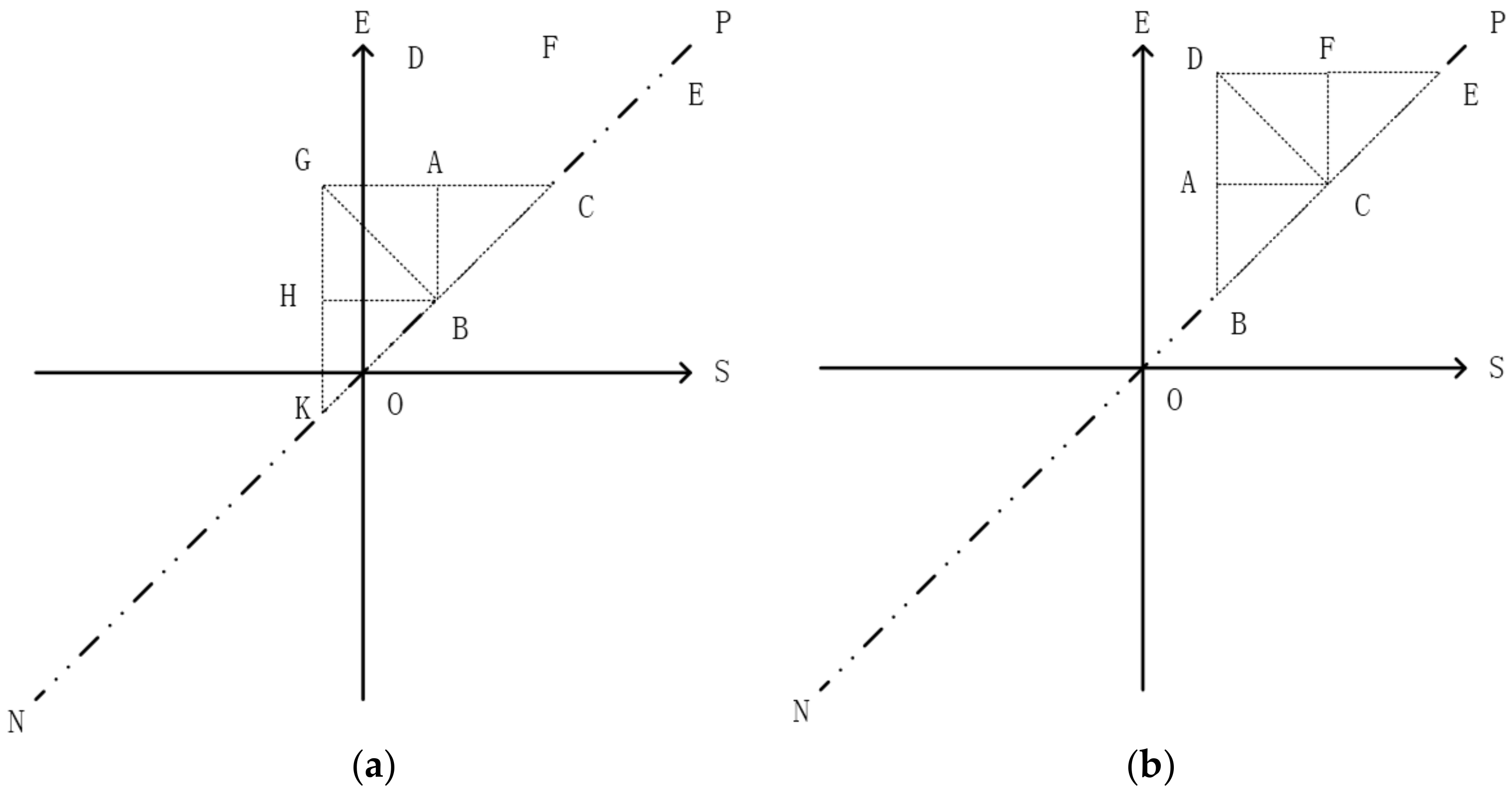
Figure 9.
DTI-Tree index structure (example of Figure 7a).
Figure 9.
DTI-Tree index structure (example of Figure 7a).
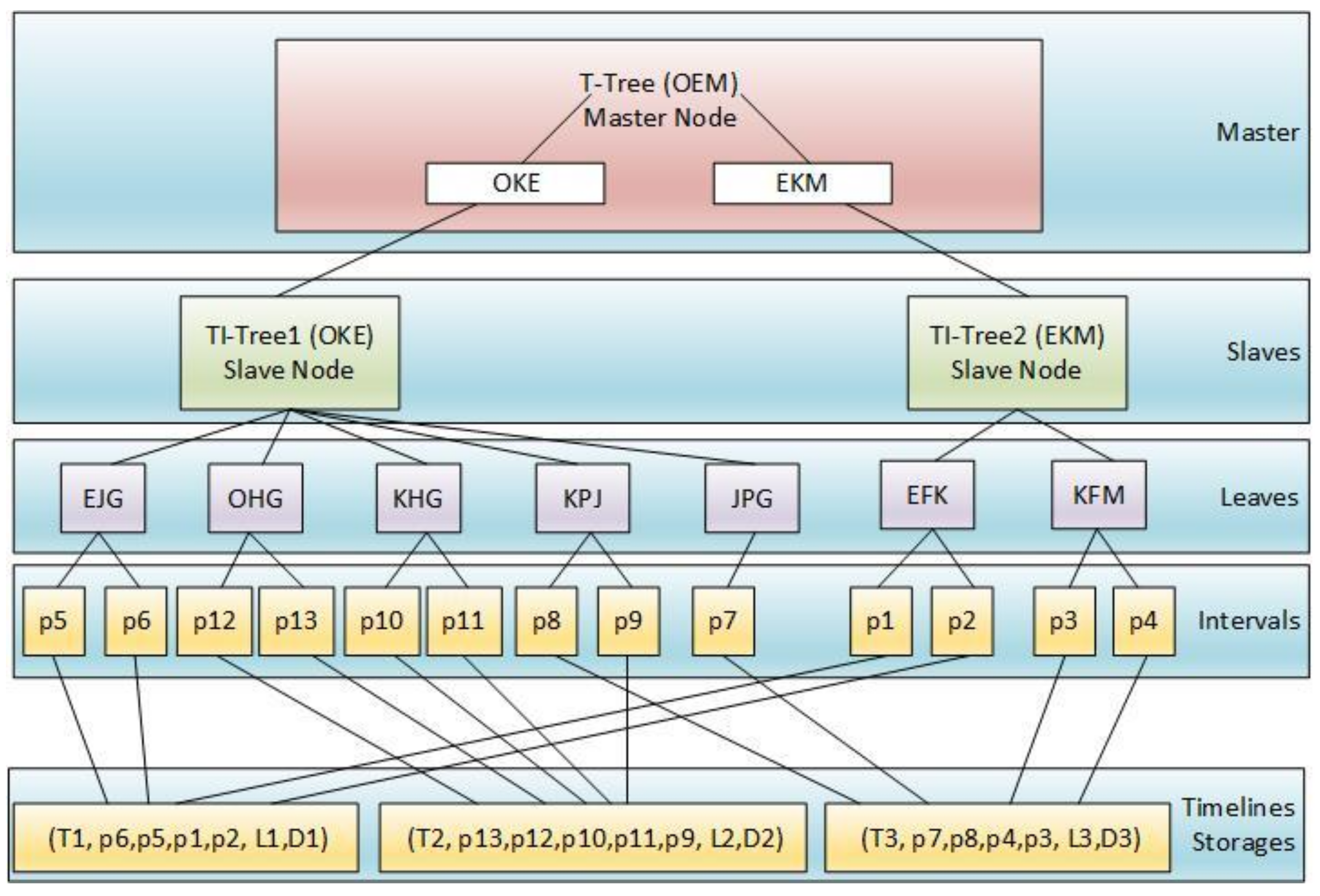
Figure 10.
DTI-Tree construction process.

Figure 11.
Main steps of similarity query.

Figure 12.
Architecture of the experimental system.

Figure 13.
Construction comparison.

Figure 14.
Insertion comparison.

Figure 15.
Similarity query performance.
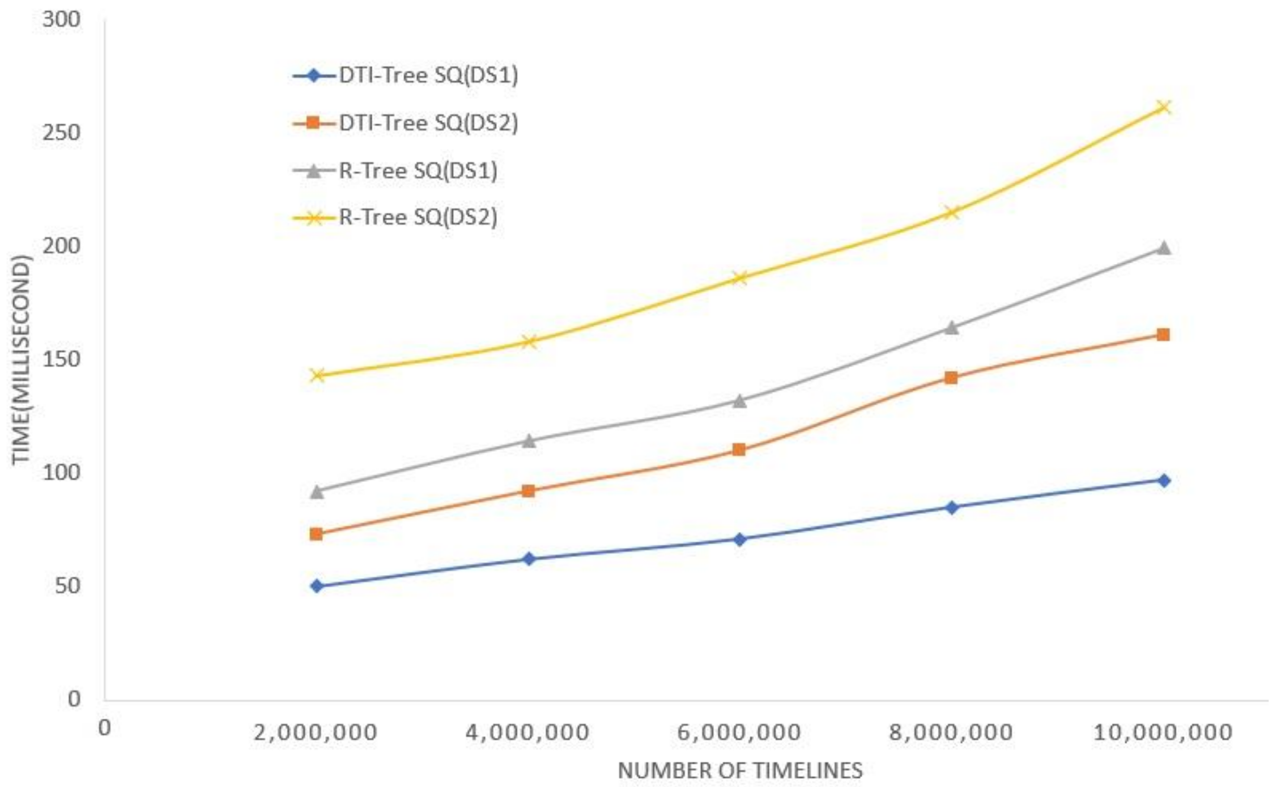
Figure 16.
Similarity query performance (label types).

Figure 17.
Similarity query performance (partitions).


Table 1.
Interval types.
| Interval Type | Expression |
|---|---|
| IT_CLOSED | [Is, Ie] |
| IT_LEFTOPEN | (Is, Ie] |
| IT_RIGHTOPEN | [Is, Ie) |
| IT_OPEN | (Is, Ie) |
Table 2.
Interval algebra relationships [9].
Table 2.
Interval algebra relationships [9].
| Operator | Definition | Result Shape |
|---|---|---|
| equals | Is = Qs and Ie = Qe | point |
| covers | Is = Qs and Ie = Qe | point, if Q is close and I is open |
| coveredBy | Is = Qs and Ie = Qe | point, if Q is open and I is close |
| Starts | Is = Qs and Qs < Ie < Qe | line |
| startedBy | Is = Qs and Ie > Qe | line |
| Meets | Is ≤ Ie = Qs ≤ Qe | line |
| metBy | Qs ≤ Qe = Is ≤ Ie | line |
| finishes | Qs < Is < Qe and Ie = Qe | line |
| finishedBy | Is < Qs and Ie = Qe | line |
| before | Is ≤ Ie < Qs ≤ Qe | region |
| After | Qs ≤ Qe < Is ≤ Ie | region |
| overlaps | Is < Qs and Qs < Ie < Qe | region |
| overlappedBy | Qs < Is < Qe and Ie>Qe | region |
| during | Qs < Is ≤ Ie < Qe | region |
| contains | Is < Qs ≤ Qe < Ie | region |
Table 3.
Common functions.
| Function | Description |
|---|---|
| cartesian | returns the cartesian product of this timeline and another one, that is, the result of all pairs of elements (a, b) where a is in this and b is in other. |
| count | returns the number of elements in the set. |
| filter | returns a new set containing only the elements that satisfy a predicate. |
| flatMap | returns a new set by first applying a function to all elements of this set, and then flattening the results. |
| foreach | applies a function f to all elements of this set. |
| groupBy | returns a set of grouped elements. |
| intervalize | convert a timeline into a set of intervals |
| min | returns the minimum element from this set as defined by the specified comparator. |
| map | returns a new set by applying a function to all elements of this set. |
| max | returns the maximum element from this set as defined by the specified comparator. |
| reduce | reduces the elements of this set using the specified commutative and associative binary operator. |
| similarity | calculate the similarity of two timelines. |
Table 4.
Parameters of TimelineGenerator.
| Parameters | Description |
|---|---|
| maxTimeValue | the maximum time value of all the timelines generated by generator, the default value is 0. |
| minTimeValue | the minimum time value of all the timelines generated by generator, the default value is 10,000. |
| timelineMinLength | the shortest length of a timeline generated by generator, the default is 10. |
| timelineMaxLength | the longest length of a timeline generated by generator, the default is 50. |
| intervalMinLength | the shortest length of an interval generated by generator, the default is 2. |
| intervalMaxLength | the longest length of an interval generated by generator, the default is 10. |
| intervalAttachment | the range of the attachment data size, the default is [1K, 2K] |
| labelTypes | the maximum types involved in the dataset generated by generator, the default value is 5. |
| numberTimelines | the total number of the timelines generated by generator, the default value is 10,000,000. |
| outputFileName | the generated timeline data file. |
© 2018 by the authors. Licensee MDPI, Basel, Switzerland. This article is an open access article distributed under the terms and conditions of the Creative Commons Attribution (CC BY) license (http://creativecommons.org/licenses/by/4.0/).
Share and Cite
MDPI and ACS Style
He, Z.; Ma, X. A Distributed Indexing Method for Timeline Similarity Query. Algorithms 2018, 11, 41. https://doi.org/10.3390/a11040041
AMA Style
He Z, Ma X. A Distributed Indexing Method for Timeline Similarity Query. Algorithms. 2018; 11(4):41. https://doi.org/10.3390/a11040041
Chicago/Turabian StyleHe, Zhenwen, and Xiaogang Ma. 2018. "A Distributed Indexing Method for Timeline Similarity Query" Algorithms 11, no. 4: 41. https://doi.org/10.3390/a11040041
Note that from the first issue of 2016, this journal uses article numbers instead of page numbers. See further details here.