Vertex Cover Reconfiguration and Beyond †

1
Department of Informatics, University of Bergen, PB 7803, N-5020 Bergen, Norway
2
School of Computer Science, University of Waterloo, Waterloo, ON N2L 3G1, Canada
3
Institute of Mathematical Sciences, Chennai 600113, India
4
Institute of Informatics, University of Warsaw, 02-097 Warsaw, Poland
*
Author to whom correspondence should be addressed.
†
This paper is an extended version of our paper published in the 25th International Symposium on Algorithms and Computation (ISAAC 2014).
‡
The work of Sebastian Siebertz is supported by the National Science Centre of Poland via POLONEZ Grant Agreement UMO-2015/19/P/ST6/03998, which has received funding from the European Union’s Horizon 2020 research and innovation programme (Marie Skłodowska-Curie Grant Agreement No. 665778).
Algorithms 2018, 11(2), 20; https://doi.org/10.3390/a11020020
Submission received: 11 October 2017
/
Revised: 2 February 2018
/
Accepted: 7 February 2018
/
Published: 9 February 2018
(This article belongs to the Special Issue Reconfiguration Problems)
Abstract
:In the Vertex Cover Reconfiguration (VCR) problem, given a graph G, positive integers k and ℓ and two vertex covers S and T of G of size at most k, we determine whether S can be transformed into T by a sequence of at most ℓ vertex additions or removals such that every operation results in a vertex cover of size at most k. Motivated by results establishing the -hardness of VCR when parameterized by ℓ, we delineate the complexity of the problem restricted to various graph classes. In particular, we show that VCR remains -hard on bipartite graphs, is -hard, but fixed-parameter tractable on (regular) graphs of bounded degree and more generally on nowhere dense graphs and is solvable in polynomial time on trees and (with some additional restrictions) on cactus graphs.
1. Introduction
Under the reconfiguration framework, we consider structural and algorithmic questions related to the solution space of a search problem . Given an instance , an optional range bounding a numerically-quantifiable property of feasible solutions for and a symmetric adjacency relation (usually polynomially-testable) on the set of feasible solutions, we can construct a reconfiguration graph for each instance of . The nodes of correspond to the feasible solutions of having , and there is an edge between two nodes whenever the corresponding solutions are adjacent under . An edge can be seen as a reconfiguration step transforming one solution into the other. Given two feasible solutions for , S and T, one can ask if there exists a walk (reconfiguration sequence) in from S to T, or for the shortest such walk. On the structural side, one can ask about the diameter of reconfiguration graph or whether it is connected with respect to some or any , fixed and fixed .
These types of reconfiguration questions have received considerable attention in recent years [1,2,3,4,5] and are interesting for a variety of reasons. From an algorithmic standpoint, reconfiguration problems model dynamic situations in which we seek to transform a solution into a more desirable one, maintaining feasibility during the process. Reconfiguration also models questions of evolution; it can represent the evolution of a genotype where only individual mutations are allowed and all genotypes must satisfy a certain fitness threshold, i.e., be feasible. Moreover, the study of reconfiguration yields insights into the structure of the solution space of the underlying problem, crucial for the design of efficient algorithms. In fact, one of the initial motivations behind such questions was to study the performance of heuristics [2] and random sampling methods [6], where connectivity and other properties of the solution space play a crucial role.
Reconfiguration problems have been studied mainly under classical complexity assumptions, with most work devoted to determining the existence of a reconfiguration sequence between two given solutions. For most -complete problems, this question has been shown to be -complete [3,7,8], while for some problems in , the reconfiguration question could be either in [3] or -complete [9]. As -completeness implies that the number of vertices in reconfiguration graphs, and therefore the length of reconfiguration sequences, can be superpolynomial in the number of vertices in the input graph, it is natural to ask whether we can achieve tractability if we restrict the length of the sequence or other properties of the problem to a fixed constant. These results motivated Mouawad et al. [10] to study reconfiguration under the parameterized complexity framework [11,12].
The Vertex Cover Reconfiguration (VCR) problem was shown to be fixed-parameter tractable when parameterized by k and -hard when parameterized by ℓ [10]; in , each feasible solution for instance G is a vertex cover of size at most k (a subset such that each edge of the graph has at least one endpoint in S) and two solutions are adjacent if one can be obtained from the other by the addition or removal of a single vertex of G. Motivated by these results, we embark on a systematic investigation of the parameterized complexity of the problem restricted to various graph classes.
In Section 4, we start by showing that the VCR problem parameterized by ℓ remains -hard when restricted to bipartite graphs. To obtain this result, we introduce the -bipartite constrained crown problem and show that it plays a central role for determining the complexity of the reconfiguration problem. As the vertex cover is solvable in polynomial time on bipartite graphs, this result provides an example of a search problem in whose reconfiguration version is -hard parameterized by ℓ, answering a question left open by Mouawad et al. [10]. In Section 5, we characterize instances of the VCR problem solvable in time polynomial in and apply this characterization to trees, graphs with no even cycles and (with some additional restrictions) to cactus graphs (we incorrectly claimed to have proved the result for cactus graphs in its full generality in an earlier version of this paper [13]). We note that a polynomial-time algorithm for even-hole-free graphs was also independently obtained by Kamiński et al. [8] for solving several variants of the closely-related independent set reconfiguration problem. Moreover, VCR is known to be -complete on graphs of bounded treewidth [14] (for some constant value of treewidth), but it remains open whether the problem is -complete already for graphs of treewidth at most two, or even outerplanar graphs. Our result on cactus graphs is a first step towards settling these questions. In Section 6, we present the first fixed-parameter tractable algorithm for VCR parameterized by ℓ on graphs of bounded degree after establishing the -hardness of the problem on four-regular graphs. Finally, we show using completely different techniques, and at the cost of a much worse running time, that VCR, as well as a host of other reconfiguration problems are fixed-parameter tractable on nowhere dense classes of graphs.
2. Preliminaries
For general graph theoretic definitions, we refer the reader to the book of Diestel [15]. Unless otherwise stated, we assume that each graph G is a simple undirected graph with vertex set and edge set , where and . The open neighbourhood of a vertex v is denoted by and the closed neighbourhood by . For a set of vertices , we define and . The subgraph of G induced by A is denoted by , where has vertex set A and edge set .
A walk of length q from to in G is a vertex sequence such that, for all , . It is a path if all vertices are distinct and a cycle if , , and is a path. A matching on a graph G is a set of edges of G such that no two edges share a vertex; we use to denote the set of vertices incident to edges in . A set of vertices is said to be saturated by if .
To avoid confusion, we refer to nodes in reconfiguration graphs, as distinguished from vertices in the input graph. We denote an instance of the vertex cover reconfiguration problem by , where G is the input graph, S and T are the source and target vertex covers, respectively, k is the maximum allowed capacity and ℓ is an upper bound on the length of the reconfiguration sequence we seek. By a slight abuse of notation, we use upper case letters to refer to both a node in the reconfiguration graph, as well as the corresponding vertex cover. For any node , the quantity corresponds to the available capacity at S. We partition into the sets (vertices common to S and T), (vertices to be removed from S in the course of reconfiguration), (vertices to be added to form T) and (all other vertices). To simplify notation, we sometimes use to denote the graph induced by the vertices in the symmetric difference of S and T, i.e., . We say a vertex is touched in the course of a reconfiguration sequence from S to T if v is either added or removed at least once. We say a vertex v, in a vertex cover S, is removable if and only if and .
Proposition 1.
For any graph G and any two vertex covers S and T of G, is bipartite. Moreover, there are no edges between vertices in and vertices in .
Proof.
None of the vertices in are included in T. Since T is a vertex cover of G, each edge of G must have an endpoint in T, and hence, must be an independent set. Similar arguments apply to and to show that there are no edges between vertices in and vertices in . ☐
Proposition 2.
For a graph G and any two vertex covers S and T of G, any vertex in must be touched an odd number of times and any vertex not in must be touched an even number of times in any reconfiguration sequence of length at most ℓ from S to T. Moreover, any vertex can be touched at most times.
3. Representing Reconfiguration Sequences
There are multiple ways of representing a reconfiguration sequence between two vertex covers of a graph G. In Section 4 and Section 5, we focus on a representation that consists of an ordered sequence of vertex covers or nodes in the reconfiguration graph. Given a graph G and two vertex covers of G, and , we denote a reconfiguration sequence from to by , where is a vertex cover of G and is obtained from by either the removal or the addition of a single vertex from for all . For any pair of consecutive vertex covers (, ) in , we say () is the successor (predecessor) of (). A reconfiguration sequence is a prefix of if .
In Section 6, we use the notion of edit sequences. We assume all vertices of G are labelled from one to n, i.e., . We let and denote the sets of addition markers and removal markers, respectively. An edit sequence is an ordered sequence of elements obtained from the full set of markers , where stands for the addition of vertex , stands for the removal of vertex and . The length of , , is equal to the total number of markers in . We let , , denote the marker at position p in . We say is a segment of whenever consists of a subsequence of with no gaps. The length of a segment is defined as the total number of markers it contains. We use the notation , , to denote the segment starting at position and ending at position . Two segments and are consecutive whenever occurs later than in and there are no gaps between and . For any pair of consecutive segments and in , we say () is the successor (predecessor) of (). Given an edit sequence , a segment of is a maximal addition segment if is a maximal subsequence of consisting of only addition markers and no gaps. Similarly, is a maximal removal segment if is a maximal subsequence of consisting of only removal markers and no gaps.
We now discuss how edit sequences relate to reconfiguration sequences. Given a graph G and an edit sequence , we use to denote the set of vertices touched in , i.e., . We let denote the set of vertices obtained after executing all reconfiguration steps in on G starting from some vertex cover S of G. We say is valid whenever every set , , is a vertex cover of G, and we say is invalid otherwise. Note that even if , is not necessarily a walk in the reconfiguration graph , as might violate the maximum allowed capacity constraint k. Hence, we let , and we say is tight whenever it is valid and .
Proposition 3.
Given a graph G and two vertex covers S and T of G, an edit sequence α is a reconfiguration sequence from S to T if and only if α is a tight edit sequence from S to T.
4. Hardness Results
In earlier work establishing the -hardness of the VCR problem parameterized by ℓ on general graphs, it was also shown that the problem becomes fixed-parameter tractable whenever [10] (as we know exactly which vertices have to be touched, it is only a question of finding the right order of additions and removals). When , we know from Proposition 2 that , since every vertex in must be touched at least once. Moreover, Proposition 1 implies that whenever , the input graph must be bipartite. It is thus natural to ask about the complexity of the problem when and the input graph is restricted to be bipartite. Since the vertex cover problem is known to be solvable in time polynomial in n on bipartite graphs, our result is, to the best of our knowledge, the first example of a problem solvable in polynomial time whose reconfiguration version is -hard.
For a graph G, a crown is a pair satisfying the following properties: (i) is an independent set of G; (ii) ; and (iii) there exists a matching in that saturates H [16,17]. H is called the head of the crown, and the width of the crown is . Crown structures have played a central role in the development of efficient kernelization algorithms for the vertex cover problem [16,17]. We define the closely-related notion of -constrained crowns and show in the remainder of this section that the complexity of finding such structures in a bipartite graph is central for determining the complexity of the reconfiguration problem.
We define a -constrained crown as a pair satisfying all properties of a regular crown with the additional constraints that and . We are now ready to introduce the -Bipartite Constrained Crown problem, or -BCC, which is formally defined as follows:
| -bipartite constrained crown | |
| Input: | A bipartite graph and two positive integers t and d |
| Parameters: | t and d |
| Question: | Does G have a -constrained crown such that and ? |
Lemma 1.
The -bipartite constrained crown is -hard even when the input graph, , is -free and all vertices in A have degree at most two.
Proof.
We give a reduction from the k-clique, known to be -hard, to the -bipartite constrained crown. For an instance of k-clique, we let and .
We first form a bipartite graph , where vertex sets X and Y contain one vertex for each vertex in and Z contains one vertex for each edge in . More formally, we set , , and . The edges in join each pair of vertices and for and the edges in join each vertex z in Z to the two vertices and corresponding to the endpoints of the edge in to which z corresponds. Since each edge either joins vertices in X and Y or vertices in Y and Z, it is not difficult to see that the vertex sets and Y form a bipartition.
By our construction, is -free; vertices in X have degree one, and since there are no double edges in G, i.e., two edges between the same pair of vertices, no pair of vertices in Y can have more than one common neighbour in Z. For an instance of -BCC, and , we claim that G has a clique of size k if and only if has a -constrained crown such that and .
If G has a clique K of size k, we set , namely the vertices in Y corresponding to the vertices in the clique. To form W, we choose , that is the vertices in X corresponding to the vertices in the clique and the vertices in Z corresponding to the edges in the clique. Clearly, H is a subset of size k of B, and W is a subset of size of A; this implies that , as required. To see why , it suffices to note that every vertex is connected to exactly one vertex , and every degree-two vertex corresponds to an edge in K whose endpoints must have corresponding vertices in H. Moreover, due to , there is a matching between the vertices of H and the vertices of W in X and, hence, a matching in that saturates H.
We now assume that has a -constrained crown such that and . It suffices to show that must be equal to k, must be equal to and, hence, must be equal to k; from this, we can conclude that the vertices in form a clique of size k in G as , requiring that edges exist between each pair of vertices in the set . Moreover, since and , a matching that saturates H can be easily found by simply picking all edges for .
To prove the sizes of H and W, we first observe that since , , and each vertex in Y has exactly one neighbour in X, we know that . Moreover, since and , we know that . If , our proof is complete, since by our construction of , H is a set of at most k vertices in the original graph G, and the subgraph induced by those vertices in G has edges. Hence, must be equal to k. Suppose instead that . In this case, since each vertex of Z has degree two, the number of neighbours of in Y is greater than k, violating the assumptions that and . ☐
We can now show the main result of this section:
Theorem 1.
VCR parameterized by ℓ and restricted to bipartite graphs is -hard.
Proof.
We give a reduction from the -bipartite constrained crown to vertex cover reconfiguration in bipartite graphs. For , an instance of the -bipartite constrained crown, and , we form such that X and Y correspond to the vertex sets A and B, connects vertices in X and Y corresponding to vertices in A and B joined by edges in G and U, V and form a complete bipartite graph . More formally, , , , , and .
We let be an instance of VCR, where and . Clearly, . We claim that G has a -constrained crown such that and if and only if there is a path of length at most from S to T.
If G has such a pair , we form a reconfiguration sequence of length at most as follows:
- (1)
- Add each vertex such that . The resulting vertex cover size is .
- (2)
- Remove vertices such that . The resulting vertex cover size is .
- (3)
- Add each vertex from V. The resulting vertex cover size is .
- (4)
- Remove each vertex from U. The resulting vertex cover size is .
- (5)
- Add each vertex removed in Phase 2. The resulting vertex cover size is .
- (6)
- Remove each vertex added in Phase 1. The resulting vertex cover size is .
The length of the sequence follows from the fact that : Phases 1 and 6 consist of at most t steps each and Phases 2, 3, 4 and 5 of at most steps each. The fact that each set forms a vertex cover is a consequence of the fact that .
For the converse, we observe that before removing any vertex , , from U, we first need to add all vertices from V. Therefore, if there is a path of length at most from S to T, then we can assume without loss of generality that there exists a node Q (i.e., a vertex cover) along this path such that:
all vertices that were touched in order to reach node Q belong to .
In other words, at node Q, the available capacity is greater than or equal to , and all edges in are still covered by U. We let and . Since , and . Moreover, since , we know that must be greater than or equal to d. Given that and we need exactly steps to add all vertices in V and remove all vertices in U, we have remaining steps to allocate elsewhere. Therefore, as , , and every vertex in must be touched at least twice (i.e., added and then removed). Combining those observations, we get:
We have just shown that G has a pair such that , , , , and , as otherwise some edge is not covered. The remaining condition for to satisfy is for to have a matching that saturates . Hall’s marriage theorem [18] states that such a saturating matching exists if and only if for every subset P of , . By a simple application of Hall’s theorem, if no such matching exists, then there exists a subgraph Z of such that . By deleting this subgraph from , we can get a new pair , which must still satisfy , , , and , since we delete more vertices from than we do from and . Finally, if does not have a matching that saturates , we can repeatedly apply the same rule until we reach a pair that satisfies all the required properties. Since , such a pair is guaranteed to exist, as otherwise every subset P of would satisfy and hence , a contradiction. ☐
5. Polynomial-Time Algorithms
In this section, we present a characterization of instances of the VCR problem solvable in time polynomial in n, and apply this characterization to trees, graphs with no even cycles (as subgraphs) and to cactus graphs (with some additional restrictions). We show how to find reconfiguration sequences of the shortest possible length and therefore ignore the parameter ℓ. Unless stated otherwise, reconfiguration sequences are represented as ordered sequences of vertex covers or nodes in the reconfiguration graph.
Definition 1.
Given two vertex covers of G, A and B, a reconfiguration sequence β from A to some vertex cover is a c-bounded prefix of a reconfiguration sequence α from A to B, if and only if all of the following conditions hold:
- (1)
- ;
- (2)
- For every node in β, ;
- (3)
- For every node in β, is obtained from its predecessor by either the removal or the addition of a single vertex in the symmetric difference of the predecessor and B;
- (4)
- No vertex is touched more than once in the course of β.
We write when such a c-bounded prefix exists.
Proposition 4.
Given two vertex covers S and T of G, if G has a vertex cover such that , then for all .
Lemma 2.
Given two vertex covers S and T of G and two positive integers k and c such that , a reconfiguration sequence α of length from S to T exists if:
- (1)
- ;
- (2)
- ; and
- (3)
- For any two vertex covers A and B of G such that and , either or , where and are vertex covers of G.
Moreover, if c-bounded prefixes can be found in time polynomial in n, then α can be found in time polynomial in n.
Proof.
We prove the lemma by induction on . When , S is equal to T, and the claim holds trivially since .
When , we know that either or . Without loss of generality, we assume and let denote the c-bounded prefix from S to . From Definition 1, we know that the size of every node in is no greater than . Therefore, the maximum allowed capacity constraint is never violated.
Since (Definition 1), by the induction hypothesis, there exists a reconfiguration sequence from to T whose length is . By appending the reconfiguration sequence from to T to the reconfiguration sequence from S to , we obtain a reconfiguration sequence from S to T.
To show that , it suffices to show that . We know that no vertex is touched more than once in , and every touched vertex belongs to (Definition 1). We let denote the set of touched vertices in , and we subdivide H into two sets and . It follows that and . Therefore, as needed.
When c-bounded prefixes can be found in time polynomial in n, the proof gives an algorithm for constructing the full reconfiguration sequence from S to T in time polynomial in n. ☐
5.1. Trees
Theorem 2.
Vertex cover reconfiguration restricted to trees can be solved in time polynomial in n.
Proof.
We let be an instance of vertex cover reconfiguration. The proof proceeds in two stages. We start by showing that when G is a tree and S and T are of size at most , we can always find one-bounded prefixes or in time polynomial in n. Therefore, we can apply Lemma 2 with to find a reconfiguration sequence of length from S to T in time polynomial in n. In the second part of the proof, we show how to handle the remaining cases where S, T or both S and T are of a size greater than .
First, we note that every forest either has a degree-zero or a degree-one vertex. Hence, trees and forests are one-degenerate graphs. Since G is a tree, is a forest and is therefore one-degenerate. To find one-bounded prefixes in , it is enough to find a vertex of degree at most one, which can clearly be done in time polynomial in n: For any two vertex covers S and T of a tree G such that , we can always find a vertex having degree at most one in . The existence of v guarantees the existence of a one-bounded prefix from either S to some vertex cover or from T to some vertex cover . When and , we have , since is obtained from S by simply removing v. When and , we have , since is obtained from S by first adding the unique neighbour of v and then removing v. Similar arguments hold when .
Therefore, combining Lemma 2 and the fact that is one-degenerate, we know that if and , a reconfiguration sequence of length from S to T can be found in time polynomial in n. Furthermore, since the length of a reconfiguration sequence can never be less than , the reconfiguration sequence given by Lemma 2 is the shortest path from S to T in the reconfiguration graph.
When S (or T) has size k and is minimal, then we have a no-instance, since neither removing, nor adding a vertex results in a k-vertex cover, and hence, S (or T) will be an isolated node in the reconfiguration graph, with no path to T (or S).
When S, T or both S and T are of size k and are non-minimal, there always exists a reconfiguration sequence from S to T, since S and T can be reconfigured to solutions and , respectively, of size less than k, to which Lemma 2 can be applied. The only reconfiguration steps from S (or T) of size k are to subsets of S of size (or to subsets of T of size ); the reconfiguration sequence obtained from Lemma 2 is thus a shortest path. Therefore, we can obtain a shortest path from S to T through a careful selection of and . There are two cases to consider:
Case (1): , , S is non-minimal and T is non-minimal. When both S and T are of size k and are non-minimal, then each must contain at least one removable vertex. Hence, by removing such vertices, we can transform S and T into vertex covers and , respectively, of size . We let u and v be removable vertices in S and T, respectively, and we set and .
- If and , then the length of a shortest reconfiguration sequence from to will be . Therefore, accounting for the two additional removals, the length of a shortest path from S to T will be equal to .
- If and , then the length of a shortest reconfiguration sequence from to will be . Since v is in , it must be removed and added back. Therefore, the length of a shortest path from S to T will be equal to . The same is true when and or when and .
- Otherwise, when , and , the length of a shortest path from S to T will be , since we have to touch two vertices in (i.e., two extra additions and two extra removals).
Case (2): , and S is non-minimal (similar arguments hold for the symmetric case where , , and T is non-minimal). Since , we only need to reduce the size of S to in order to apply Lemma 2. Since S is non-minimal, it must contain at least one removable vertex. We let u be a removable vertex in S, and we set .
- If , then the length of a shortest reconfiguration sequence from to T will be . Therefore, accounting for the additional removal, the length of a shortest path from S to T will be equal to .
- If , then the length of a shortest reconfiguration sequence from to T will be . Since v is in , it must be removed and added back. Therefore, the length of a shortest path from S to T will be equal to .
As there are at most pairs of removable vertices in S and T to check for Case (1), we can exhaustively try all pairs and choose one that minimizes the length of a reconfiguration sequence. Similarly, there are at most k removable vertices to check in Case (2). Consequently, vertex cover reconfiguration on trees can be solved in time polynomial in n. ☐
5.2. Cactus Graphs
A cactus graph G [19] is a connected graph in which every edge belongs to at most one cycle. We let denote the set of all cycles in G. We say vertex is a join vertex if v belongs to a cycle and .
The following proposition is a consequence of the fact that a maximal matching of a cactus graph G can contain an edge from each cycle in .
Proposition 5.
For a cactus graph G, the number of cycles in G is bounded above by the size of a maximum matching , i.e., .
The next proposition is a consequence of the fact that for any cactus graph G, we can obtain a spanning tree of G by removing a single edge from every cycle in G.
Proposition 6.
For a cactus graph G and a spanning tree of G, the total number of edges in G is equal to the number of edges in plus the total number of cycles in G, i.e., .
Any graph with no even cycles (as subgraphs) is a cactus graph [20]. For a graph G with no even cycles and any two vertex covers, S and T, of G, we know that must be a forest, i.e., a bipartite graph with no even cycles (Proposition 1). Proposition 7 follows from the fact that in the proof of Theorem 2, the fact that G is a tree is used only to determine that must be a forest. Therefore, using the same proof as in Theorem 2, we can show:
Proposition 7.
Vertex cover reconfiguration on graphs with no even cycles can be solved in time polynomial in n.
In the remainder of this section, we generalize Proposition 7 to all cactus graphs assuming that the given vertex covers S and T are of size at most . To do so, we first show, in Lemmas 3 and 4, that the third condition of Lemma 2 is satisfied for cactus graphs with . In Lemma 5, we show how two-bounded prefixes can be found in time polynomial in n, which leads to Theorem 3. We note that a similar result was proven independently by Ito et al. [21] via completely different methods.
Lemma 3.
Given two vertex covers S and T of G, there exists a vertex cover (or ) of G such that (or ) if one of the following conditions holds:
- (1)
- has a vertex () such that ; or
- (2)
- there exists a cycle Y in such that all vertices in () have degree exactly two in .
Moreover, both conditions can be checked in time polynomial in n, and when one of them is true, the corresponding two-bounded prefix can be found in time polynomial in n.
Proof.
First, we note that checking for Condition (1) can be accomplished in time polynomial in n by simply inspecting the degree of every vertex in . The total number of cycles satisfying condition (2) is linear in the number of degree-two vertices in . Therefore, we can check for Condition (2) in time polynomial in n by a simple breadth-first search starting from every degree-two vertex in .
If has a vertex of degree zero, we let denote the vertex cover obtained by simply removing v from S. It is easy to see that the reconfiguration sequence from S to is a zero-bounded prefix and can be found in time polynomial in n.
Similarly, if has a vertex of degree one, we let denote the node obtained by the addition of the single vertex in followed by the removal of v. The reconfiguration sequence from S to is a one-bounded prefix and can be found in time polynomial in n.
For the second case, we let Y be a cycle in , and we partition the vertices of the cycle into two sets; and . Since is bipartite, we know that . Since all vertices in have degree exactly two in , it follows that . Therefore, a reconfiguration sequence from S to some vertex cover that adds all vertices in (one by one) and then removes all vertices in (one by one) will satisfy Conditions (1), (3) and (4) from Definition 1 for any value of c. For , such a sequence will not satisfy Condition (2) if the cycle has at least six vertices (i.e., ). However, using the fact that every vertex in has degree exactly two in , we can find a reconfiguration sequence from S to in which no vertex cover has a size greater than . To do so, we restrict our attention to . Since Y is an even cycle, we can label all the vertices of Y in clockwise order from zero to such that all vertices in receive even labels. The reconfiguration sequence from S to starts by adding the two vertices labelled 1 and . After doing so, the vertex labelled 0 is removed. Next, to remove the vertex labelled 2, we only need to add the vertex labelled 3. The same process is repeated for all vertices with even labels up to . Finally, when we reach the vertex labelled , both of its neighbours will have already been added, and we can simply remove it. Hence, we have a two-bounded prefix from S to , and it is not hard to see that finding this reconfiguration sequence can be accomplished in time polynomial in n.
When the appropriate assumptions hold, we can show the symmetric case using similar arguments. ☐
Lemma 4.
If G is a cactus graph and S and T are two vertex covers of G, then there exists a vertex cover (or ) of G such that (or ).
Proof.
We assume that , as we can swap the roles of S and T whenever . We observe that every connected component of is a cactus graph since every induced subgraph of a cactus graph is also a cactus graph. Since we assume , at least one connected component X of must satisfy .
To prove the lemma, we show that if neither condition of Lemma 3 applies to X, it must be the case that , contradicting our assumption. To simplify the notation, we assume without loss of generality that is connected, as we can otherwise set . The proof proceeds in two steps. First, we show that if Condition (1) of Lemma 3 is not satisfied, then must have at least one vertex of degree at most two in . In the second step, we show that if both Conditions (1) and (2) of Lemma 3 are not satisfied, then , which completes the proof by contradiction.
Since is a cactus graph, we can apply Propositions 5 and 6 to get:
Moreover, since is bipartite (Proposition 1), the size of a maximum matching in is less than or equal to . Therefore:
If the minimum degree in of any vertex in is three or more, then and thus , contradicting our assumption that . Hence, must have at least one vertex of degree two in .
Next, we show that if has no vertex such that and no cycle Y such that all vertices in have degree exactly two in , then . We let denote the set of vertices in having degree x in . Since has no vertex such that , we know that cannot be empty. In addition, since there is no cycle Y in such that all vertices in have degree exactly two in , any cycle involving a vertex in must also include a vertex from . It follows that is a feedback vertex set (a set whose removal destroys all cycles) of , and is a forest.
We let denote the maximum degree in of any vertex in . Since each edge in has one endpoint in ,
and since each vertex in is in some and using (1), we can rewrite (4) as:
To bound , we note that since no edge can belong to more than one cycle in a cactus graph, any vertex can be involved in at most cycles. Combining this observation with the fact that any cycle involving a vertex in must also include a vertex from , we have:
Finally, by rewriting as and given that for , we obtain the desired bound:
This completes the proof. ☐
Lemma 5.
If G is a cactus graph and S and T are vertex covers of G, then finding a two-bounded prefix from S to some vertex cover (or from T to some vertex cover ) of G can be accomplished in time polynomial in n.
Proof.
To find a two-bounded prefix from S to some vertex cover (or from T to some vertex cover ), we simply need to satisfy one of the conditions of Lemma 3, which can both be checked in time polynomial in n. Since is a cactus graph, we know from Lemma 4 that one of them must be true. ☐
Theorem 3.
If S and T are of size at most , then vertex cover reconfiguration on cactus graphs can be solved in time polynomial in n.
Proof.
From Lemma 4, we know that for any cactus graph G and two vertex covers S and T of G, then either or , where and are some vertex covers of G. In addition, Lemma 5 shows that such two-bounded prefixes can be found in time polynomial in n. By combining these facts, we can now apply Lemma 2. That is, if and , a reconfiguration sequence of length from S to T can be found in time polynomial in n. ☐
It remains open whether we can solve the VCR problem in polynomial time on cactus graphs without any restrictions on the size of S and T. For instance, it is unclear if we can always determine (in polynomial time) whether a vertex cover of size can be transformed into a vertex cover of size and, if so, whether we can find the shortest reconfiguration sequence.
6. Algorithms
In this section, we first focus on vertex cover reconfiguration on graphs of bounded degree. We start by showing that vertex cover reconfiguration is -hard on graphs of degree at most d, for any , by proving -hardness on 4-regular graphs. The proof is based on the observation that the reconfiguration version of the problem is at least as hard as the compression version:
| Vertex cover compression | |
| Input: | A graph and a vertex cover C of G such that |
| Parameters: | k |
| Question: | Does G have a vertex cover of size ? |
The -hardness result relies on the representation of reconfiguration sequences as edit sequences. Next, we give an algorithm for vertex cover reconfiguration on graphs of bounded degree. Finally, we show that a host of graph reconfiguration problems definable in first-order logic is fixed-parameter tractable on nowhere dense classes of graphs.
6.1. Compression via Reconfiguration
Theorem 4.
Vertex cover reconfiguration is at least as hard as vertex cover compression.
Proof.
We give a reduction from the latter to the former. For , an instance of vertex cover compression, we let and form , where consists of the disjoint union of a copy of G and a biclique . Formally, we have:
We let be an instance of vertex cover reconfiguration, where and . Clearly, and both S and T are vertex covers of . We claim that G has a vertex cover of size if and only if there is a reconfiguration sequence of length or less from S to T.
Before we can remove any vertex from , we need to add all k vertices from . However, , which violates the maximum allowed capacity. Therefore, if there is a reconfiguration sequence from S to T, then one of the vertex covers in the sequence must contain at most vertices. Of those vertices, k vertices correspond to the vertices in and cover only the edges in . Thus, the remaining vertices must be in and should cover all the edges in . By our construction of , these vertices correspond to a vertex cover of G.
Similarly, if G has a vertex cover such that , then the following reconfiguration sequence transforms S to T: add all vertices of , remove all vertices of C, add all vertices of , remove all vertices from and finally add back all vertices of C and remove those of . The length of this sequence is equal to whenever and is shorter otherwise. ☐
6.2. -Hardness on Four-Regular Graphs
We are now ready to show that vertex cover reconfiguration remains -hard even if the input graph is restricted to be four-regular. We use the same ideas as we did in the previous section. Since vertex cover remains -hard on four-regular graphs [22] and any algorithm that solves the vertex cover compression problem can be used to solve the vertex cover problem, we get the desired result. The main difference here is that we need to construct a gadget, , that is also four-regular. We describe in terms of several component subgraphs, each playing a role in forcing the reconfiguration of vertex covers.
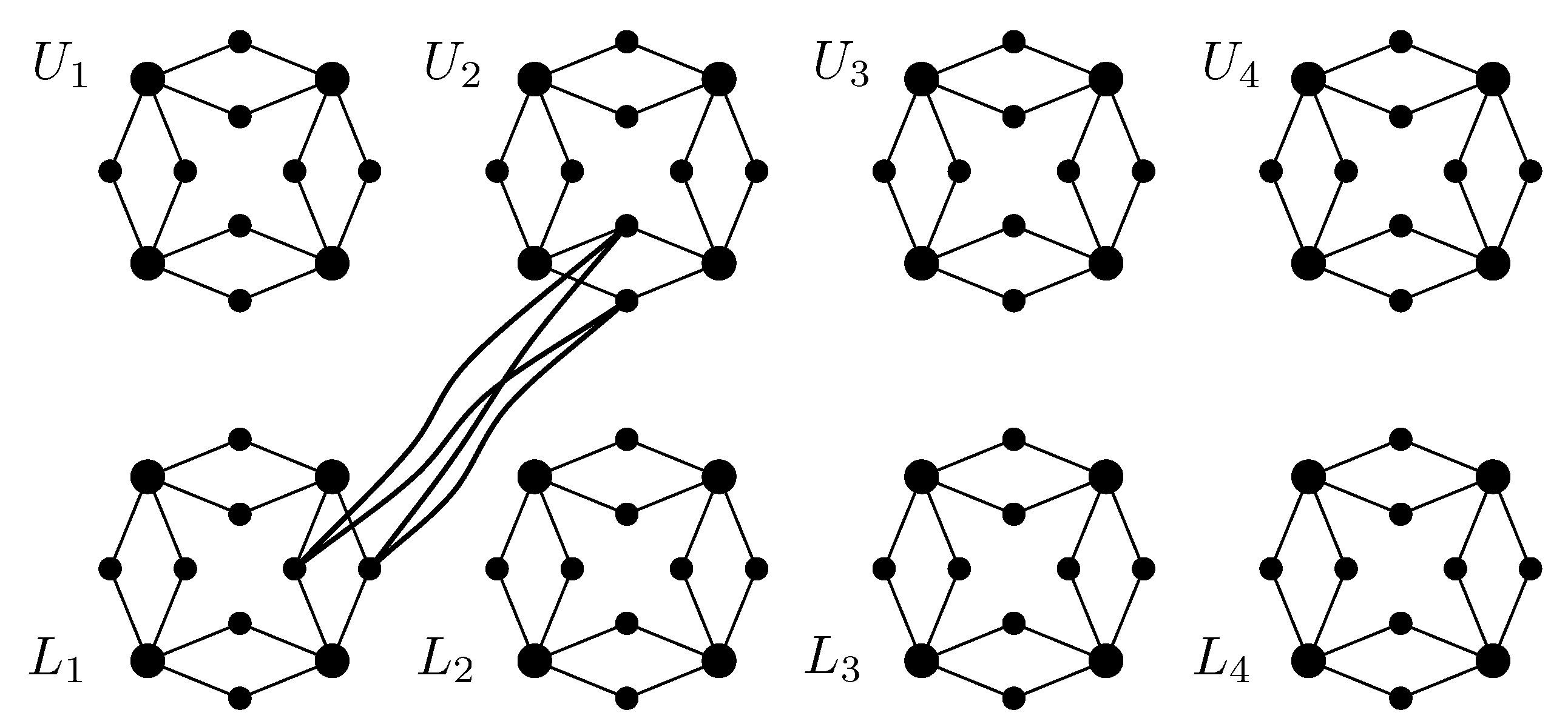
A k-necklace, , is a graph obtained by replacing every edge in a cycle on k vertices by two vertices and four edges. For convenience, we refer to every vertex on the original cycle as a bead and every new vertex in the resulting graph as a sequin. The resulting graph has k beads each of degree four and sequins each of degree two. Every two sequins that share the same neighbourhood in a k-necklace are called a sequin pair. We say two beads are adjacent whenever they share exactly two common neighbours. Similarly, we say two sequin pairs are adjacent whenever they share exactly one common neighbour. Every two adjacent beads (sequin pairs) are linked by a sequin pair (bead).
The graph consists of copies of a k-necklace. We let and denote the first and second k copies, respectively; for convenience, we use the terms “upper” and “lower” to mean “in U” and “in L”, respectively. We let and denote the j-th beads of necklace and , respectively, where and . Beads on each necklace in are numbered consecutively in “clockwise order” from one to k. For every two adjacent beads and , where , we let denote the sequin pair that links both beads.
For each sequin pair , we add four edges to form a (a joining biclique) with the pair , for all (Figure 1); we say that sequin pairs and are joined. All joining bicliques in are vertex disjoint. The total number of vertices in is . Every vertex has degree exactly four; every bead is connected to four sequins from the same necklace, and every sequin is connected to two beads from the same necklace and two other sequins from a different necklace. We let S be the set containing all upper beads and lower sequins, whereas T contains all lower beads and upper sequins. Formally, and . Each set contains vertices, that is half the vertices in .
Proposition 8.
S and T are minimum vertex covers of .
Proof.
We need at least vertices to cover the edges in the vertex disjoint joining bicliques contained in . Moreover, any minimal vertex cover C of that includes a vertex v from a sequin pair , where , must also include w. Otherwise, the two beads linking to its adjacent sequin pairs must be in C to cover the edges incident on w, making v removable. Hence, any minimal vertex cover C of must include either one or both sequin pairs in a joining biclique. We let x denote the number of joining bicliques from which two sequin pairs are included in C. Similarly, we let y denote the number of joining bicliques from which only one sequin pair is included in C. Hence, and . When , and C cannot be a minimum vertex cover, as S and T are both vertex covers of of size . When , we are left with at least y uncovered edges incident to the sequin pairs not in C. Those edges must be covered using at least y beads and, hence, . If we assume , we get a contradiction since and . Therefore, S and T must be minimum vertex covers of . ☐
To prove the next two results, we consider the representation of reconfiguration sequences as edit sequences. Since S is a minimal vertex cover of , cannot start with a vertex removal. Since is a vertex cover of , and S and T are minimum vertex covers of , cannot end with a vertex addition. Moreover, if , then must touch every vertex in exactly once.
Proposition 9.
Any (valid) edit sequence of length from S to T can be converted into a (valid) edit sequence α from S to T such that , , for all , and any two vertices u and v from the same sequin pair in are either added in the same maximal addition segment or removed in the same maximal removal segment of α. Consequently, .
Proof.
Both vertices in a sequin pair share the same neighbourhood. Hence, when u is removed, all of its neighbours must have been added, making v also removable. Moreover, since every vertex is touched exactly once in , none of the neighbours of u and v will be touched in after the removal of u. Therefore, if v is not removed in the same maximal removal segment as u, then we obtain by shifting the removal of v, so that it happens immediately after the removal of u. It is not hard to see that and , for all .
For the case of additions, if only u is added in some maximal addition segment , then none of its neighbours can yet be removed. Let be the maximal addition segment in which v is added (which occurs after in ). We obtain by shifting the addition of u from to . ☐
Lemma 6.
There exists a function of k, , such that is a yes-instance and is a no-instance of vertex cover reconfiguration for . Moreover, .
Proof.
To show that such an exists, we first prove the lower bound by showing that any valid edit sequence of length from S to T must have some prefix where the number of vertex additions minus the number of vertex removals is at least , i.e., . In fact, we will show that the aforementioned property holds for any valid edit sequence of length in which two vertices from the same sequin pair are always added or removed in the same maximal addition or removal segment, respectively. Considering only such sequences is sufficient because, from Proposition 9, we know that any sequence of length can be transformed into such a sequence so that , for all . In other words, if has no prefix with (but does), then , a contradiction.
We let position x, , be the smallest position such that contains exactly vertex removals. Those vertices correspond to a set , as touches every vertex exactly once. The claim is that must contain at least vertex additions. We let denote the set of added vertices in . Since , we complete the proof of the lower bound by showing that . To do so, we show that for any of size , contains at least vertices.
In what follows, we restrict our attention to the bipartite graph , and we let and denote the two partitions of Z. We subdivide into two sets: contains upper beads, and contains lower sequins. Since every vertex in has four neighbours in and adjacent beads share exactly two neighbours, we have , and equality occurs whenever contains beads from the same two upper necklaces. Whenever contains fewer than beads and consists of connected components, at least one bead from each component (except possibly the first) will be adjacent to at most one other bead in the same component. Therefore, .
Proposition 9 implies that will always contain both vertices of any sequin pair. Since we are only considering vertices in , some sequins in might be missing the other sequin in the corresponding pair. However, all the neighbours of the sequin pair have to be in , so we assume without loss of generality that vertices in can be grouped into sequin pairs. Every sequin pair in has four neighbours in . Adjacent sequin pairs share exactly one neighbour. Hence, , and equality occurs whenever contains k sequin pairs of a single lower necklace. Whenever contains fewer than k sequin pairs and consists of connected components, at least one sequin pair from each component will be adjacent to at most one other sequin pair in the same component. Therefore, .
Combining the previous observations, we know that when either or is empty, , as needed. When both are not empty, we let . Hence, , and we rewrite it as:
We now bound the size of I. Note that I can only contain upper sequin pairs joined with sequin pairs in . As every sequin pair in has either zero or two neighbours in I, . Moreover, for every two sequin pairs in having two neighbours in I, there must exist at least one vertex in , which implies . Finally, whenever a sequin pair has two neighbours in I, then , as at least one bead neighbouring the sequin pair joined with p must be in . Every other sequin pair , , with two neighbours in I will force at least one additional connected component in either or since contains a single joining biclique between any two necklaces. Therefore, the total number of connected components is . Putting it all together, we get:
Therefore, is a vertex cover of of size at least , as needed.
To show the upper bound, we show that is a yes-instance by providing an actual reconfiguration sequence:
- (1)
- Add all k beads in . Since S is a vertex cover of , we know that the additional k beads will result in a vertex cover of size .
- (2)
- Add both vertices in , and remove both vertices in . The removal of both vertices in is possible since we added all their neighbours in (Step (1)) and . The size of a vertex cover reaches after the additions and then drops back to .
- (3)
- Repeat Step (2) for all sequin pairs and for . The size of a vertex cover is again once Step (3) is completed. Step (2) is repeated a total of k times. After every repetition, we have a vertex cover of since all beads in were added in Step (1), and the remaining neighbours of each sequin pair in are added prior to the removals.
- (4)
- Add both vertices in , and remove vertex .
- (5)
- Add and . At this point, the size of a vertex cover is .
- (6)
- Remove both vertices in .
- (7)
- Repeat Steps (4), (5) and (6) until all beads in have been added and the sequin pairs removed. When we reach the last sequin pair in , was already added, and hence, we gain a surplus of one, which brings the vertex cover size back to .
- (8)
- Repeat Steps (4) to (7) for every remaining necklace in L.
Since every vertex in is touched exactly once, we know that . In the course of the described reconfiguration sequence, the maximum size of any vertex cover is . Hence, . This completes the proof. ☐
It would be interesting to close the gap on , but the existence of such a value is enough to prove the main theorem of this section.
Theorem 5.
Vertex cover reconfiguration is -hard on four-regular graphs.
Proof.
We prove the result by a reduction from vertex cover compression to vertex cover reconfiguration where the input graph is restricted to be four-regular in both cases. For , an instance of vertex cover compression, we form . We let be an instance of vertex cover reconfiguration, where and , and is the value whose existence was shown in Lemma 6.
Clearly, and both S and T are vertex covers of . We claim that G has a vertex cover of size if and only if there is a reconfiguration sequence of length or less from S to T.
We know from Lemma 6 that the reconfiguration of requires at least available capacity. However, , which violates the maximum allowed capacity. Therefore, if there is a reconfiguration sequence from S to T, then one of the vertex covers in the sequence must contain at most vertices. By Proposition 8, we know that of those vertices are needed to cover the edges in . Thus, the remaining vertices must be in and should cover all edges in . By construction of , these vertices correspond to a vertex cover of G.
Similarly, if G has a vertex cover such that , then the following reconfiguration sequence transforms S to T: add all vertices of , remove all vertices of C, apply the reconfiguration sequence whose existence was shown in Lemma 6 to and finally add back all vertices of C and remove those of . The length of this sequence is equal to whenever and is shorter otherwise. ☐
6.3. Algorithm for Graphs of Bounded Degree
In this section, we prove that vertex cover reconfiguration parameterized by ℓ is fixed-parameter tractable for graphs of degree at most d. Our algorithm is randomized and based on a variant of the colour-coding technique [23] that is particularly useful in designing parameterized algorithms on graphs of bounded degree. The technique, known in the literature as random separation [24], boils down to a simple, but fruitful observation that in some cases, if we randomly colour the vertex set of a graph using two colours, the solution or vertices we are looking for are appropriately coloured with high probability. In our case, we want to make sure that the set of touched vertices gets highlighted. We note that our algorithm can easily be derandomized using standard techniques [25].
We start with an instance of VCR, with G having degree at most d. Recall that we partition into the sets , , , and the independent set . We colour independently every vertex of G using one of two colours, say red and blue (denoted by and ), with probability . We let denote the resulting random colouring. Suppose that is a yes-instance, and let denote a reconfiguration sequence from S to T of length at most ℓ. We say that the colouring is successful if both of the following conditions hold:
- Every vertex in is coloured red; and
- Every vertex in is coloured blue.
Observe that and are disjoint. Therefore, the two aforementioned conditions are independent. Moreover, since the maximum degree of G is d, we have . Consequently, the probability that is successful is at least:
Let denote the set of vertices coloured red and denote the set of vertices coloured blue. Moreover, we let , …, denote the set of connected components of . The main observation now is the following:
Proposition 10.
If χ is successful, then , has a non-empty intersection with at most ℓ connected components of , and each one of those components consists of at most ℓ vertices.
Proof.
The fact that follows from the observation that every vertex in must be added or removed at least once and no vertex in is ever added or removed. In other words, if is removed, then all of its untouched neighbours must be in . Similarly, if is added, then prior to being added, all of its untouched neighbours must be in .
Since , we know that consists of at most ℓ connected components (each of size at most ) and consists of at most ℓ components (each of size at most ℓ). Let C be a connected component of such that . We claim that we can safely ignore (and hence delete) this component when is successful. Suppose to the contrary that . Since is successful, it must be the case that every vertex in is coloured blue. However, we know that there exists at least one vertex in that is coloured red (since C is a connected component of and all vertices in C are coloured red). As we have obtained a contradiction, we can conclude that when is successful, can intersect at most ℓ connected components of , and none of those components can be of a size greater than ℓ, as claimed. ☐
Given Proposition 10, we can safely assume that every connected component of consists of at most ℓ vertices (as the remaining components can be ignored when is successful). For simplicity, let us first assume that is connected. Thus, if is successful, then there exists a single component in , say , such that , and . Therefore, we can simply enumerate all possible sequences of length at most ℓ and make sure that at least one of them is the required reconfiguration sequence from S to T. This brute-force testing can be accomplished in time .
Let us now consider the general case when is not necessarily connected. We say a component C of is important if . There are at most ℓ important components. Hence, we only need to bound the number of unimportant components. To that end, we partition the unimportant components of into equivalence classes with respect to the following relation ≃:
Proposition 11.
The total number of graphs with at most ℓ vertices is at most , and therefore, the equivalence relation ≃ has at most equivalence classes.
Assume that some equivalence class contains more than ℓ unimportant components. We claim that retaining only ℓ of them is enough. To see why, it is enough to note that intersects with at most ℓ of those components; they are all isomorphic; and the neighbours of any such component are contained in . Putting it all together, we know that we have at most equivalence classes, each with at most ℓ components, and each component is of size at most ℓ. Hence, we can guess the sequence from S to T in time (testing whether two graphs with ℓ vertices are isomorphic can be accomplished naively in time ).
We have proven that the probability that is successful is at least . Hence, to obtain a Monte Carlo algorithm with false negatives, we repeat the above procedure times and obtain the following result:
Theorem 6.
There exists a one-sided error Monte Carlo algorithm with false negatives that solves the vertex cover reconfiguration problem on graphs of degree at most d in time .
6.4. Algorithm for Nowhere Dense Graphs
In this section, we present a more general result, showing that the reconfiguration variant of every first-order definable optimization problem parameterized by ℓ is fixed-parameter tractable on every fixed nowhere dense class of graphs.
Let us quickly recall the necessary definitions from logic. For our purpose, it suffices to consider first-order logic over the vocabulary of coloured graphs. We refer to the textbook [26] for extensive background on logic.
Let be two unary relation symbols and E a binary relation symbol. We call the vocabulary of graphs with two colours A and B. First-order formulas over the vocabulary of coloured graphs are formed from atomic formulas , , and , where are variables (we assume that we have an infinite supply of variables), by the usual Boolean connectives ¬ (negation), ∧ (conjunction) and ∨ (disjunction) and existential and universal quantification , respectively. The free variables of a formula are those not in the scope of a quantifier, and we write to indicate that the free variables of the formula are among . To define the semantics, we inductively define a satisfaction relation ⊨. Let G be a graph and . For simplicity, we do not distinguish between A as a symbol and A as a set. For a formula , and , means that G satisfies if the free variables are interpreted by . If is atomic, then if . Similarly, if , then if . The meanings of the equality symbol, the Boolean connectives and the quantifiers are the usual ones.
Let be a first-order formula that has a free set variable X. For example, the vertex cover problem is defined by the formula:
As another example, we can define dominating sets by the formula:
and independent sets by the formula:
Naturally, we can define a reconfiguration variant for each such formula . Given two sets , we ask for a sequence , and such that for all intermediate configurations . We call the corresponding decision problem -reconfiguration, and we refer to a solution of a problem instance as a -reconfiguration sequence.
Nowhere dense graph classes were introduced by Nešetřil and Ossona de Mendez [27] as a very general model of uniform sparseness in graphs. We refer to the textbook [28] for the formal definition of the notion of nowhere denseness and for more background on its theory. For our purpose, it is sufficient to note that most familiar classes of sparse graphs are nowhere dense, e.g., every proper minor closed class and every class of bounded degree is nowhere dense. We will prove the following theorem.
Theorem 7.
Let be a first-order formula over the vocabulary of graphs with a free set variable; let be a nowhere dense class of graphs; let be a real; and let be an integer. Then, there exists a constant and an algorithm that, given an n-vertex graph and two sets with , , decides whether there exists a φ-reconfiguration sequence of length at most ℓ in time .
Proof.
Our proof is based on a result of Grohe, Kreutzer and Siebertz [29], which states that for every first-order formula (without free variables), every nowhere dense class of graphs and every real , there exists a constant , such that given an n-vertex graph , one can decide in time whether holds in G.
In order to approach the -reconfiguration problem, we want to write a formula over the vocabulary of graphs with two colours S and T without free variables, which expresses the existence of a -reconfiguration sequence of length at most ℓ. We will guarantee that the length of is bounded by a function depending only on ℓ (and on , though only as a fixed constant). Then, by fixing any and using the result of [29], we conclude that -Reconfiguration is fixed-parameter tractable parameterized by ℓ on every nowhere dense class .
The formula simply states the existence of a sequence of ℓ elements that will be added or removed in the course of the reconfiguration. For each initial sequence of length of these ℓ guesses, we state in that the formula is satisfied for the set S modified according to the first i operations. Finally, we state that the reconfiguration leads to the set T. The precise formula is cumbersome to write; however, we expect that the reader is convinced that we can express the desired statement in first-order logic once we have stated how to handle a single addition and removal of a vertex. To state that a vertex is added to the set S, we write the formula:
where is obtained from by replacing every atom for a variable x by the formula . If we now want to remove a vertex, we extend the formula to the formula:
where is the formula obtained from by replacing every atom by the formula , and is obtained from by replacing by . Similarly, we can handle any sequence of additions and removals of vertices of length at most ℓ and form a big disjunction over all such sequences to obtain the final formula . ☐
7. Conclusions
To the best of our knowledge, our results constitute the first in-depth study of the VCR problem parameterized by the length of a reconfiguration sequence. We showed that even though the vertex cover problem is solvable in polynomial time on bipartite graphs, VCR remains -hard. On the tractable side, we showed that VCR is solvable in polynomial time for trees, as well as graphs with no even cycles and is fixed-parameter tractable for graphs of bounded degree. It remains open whether we can solve VCR in polynomial time on cactus graphs without any restrictions on the size of S and T. Finally, we believe that the techniques used in both our hardness proofs and positive results can be extended to cover a host of graph deletion problems defined in terms of hereditary graph properties [10]. It also remains to be seen whether our results can be extended to a larger class of sparse graphs, e.g., biclique-free graphs.
Acknowledgments
The authors would like to thank Daniel Lokshtanov for fruitful discussions that greatly helped improve the presentation of some of the results.
Author Contributions
All the authors contributed equally to this work.
Conflicts of Interest
The authors declare no conflict of interest.
References
- Fricke, G.; Hedetniemi, S.M.; Hedetniemi, S.T.; Hutson, K.R. γ-Graphs of Graphs. Discuss. Math. Graph Theory 2011, 31, 517–531. [Google Scholar] [CrossRef]
- Gopalan, P.; Kolaitis, P.G.; Maneva, E.N.; Papadimitriou, C.H. The connectivity of boolean satisfiability: Computational and structural dichotomies. SIAM J. Comput. 2009, 38, 2330–2355. [Google Scholar] [CrossRef]
- Ito, T.; Demaine, E.D.; Harvey, N.J.A.; Papadimitriou, C.H.; Sideri, M.; Uehara, R.; Uno, Y. On the complexity of reconfiguration problems. Theor. Comput. Sci. 2011, 412, 1054–1065. [Google Scholar] [CrossRef]
- Ito, T.; Kawamura, K.; Ono, H.; Zhou, X. Reconfiguration of list L(2, 1)-labelings in a graph. In Proceedings of the 23rd Annual International Symposium on Algorithms and Computation, Taipei, Taiwan, 19–21 December 2012; pp. 34–43. [Google Scholar]
- Kamiński, M.; Medvedev, P.; Milanič, M. Shortest paths between shortest paths. Theor. Comput. Sci. 2011, 412, 5205–5210. [Google Scholar] [CrossRef]
- Cereceda, L.; van den Heuvel, J.; Johnson, M. Connectedness of the graph of vertex-colourings. Discret. Math. 2008, 308, 913–919. [Google Scholar] [CrossRef] [Green Version]
- Ito, T.; Kamiński, M.; Demaine, E.D. Reconfiguration of list edge-colourings in a graph. Discrete Appl. Math. 2012, 160, 2199–2207. [Google Scholar] [CrossRef]
- Kamiński, M.; Medvedev, P.; Milanič, M. Complexity of independent set reconfigurability problems. Theor. Comput. Sci. 2012, 439, 9–15. [Google Scholar] [CrossRef]
- Bonsma, P. The complexity of rerouting shortest paths. In Proceedings of the International Symposium on Mathematical Foundations of Computer Science, Bratislava, Slovakia, 27–31 August 2012; pp. 222–233. [Google Scholar]
- Mouawad, A.E.; Nishimura, N.; Raman, V.; Simjour, N.; Suzuki, A. On the Parameterized Complexity of Reconfiguration Problems. Algorithmica 2017, 78, 274–297. [Google Scholar] [CrossRef]
- Downey, R.G.; Fellows, M.R. Parameterized Complexity; Springer-Verlag: New York, NY, USA, 1997. [Google Scholar]
- Downey, R.G.; Fellows, M.R. Texts in Computer Science. In Fundamentals of Parameterized Complexity; Springer: Berlin, Germany, 2013. [Google Scholar]
- Mouawad, A.E.; Nishimura, N.; Raman, V. Vertex Cover Reconfiguration and Beyond. In Proceedings of the Algorithms and Computation—25th International Symposium, ISAAC 2014, Jeonju, Korea, 15–17 December 2014; pp. 452–463. [Google Scholar]
- Wrochna, M. Reconfiguration in bounded bandwidth and tree-depth. J. Comput. Syst. Sci. 2018, 93, 1–10. [Google Scholar] [CrossRef]
- Diestel, R. Graph Theory; Electronic Ed.; Springer-Verlag: Berlin, Germany, 2005. [Google Scholar]
- Abu-Khzam, F.N.; Collins, R.L.; Fellows, M.R.; Langston, M.A.; Suters, W.H.; Symons, C.T. Kernelization Algorithms for the Vertex Cover Problem: Theory and Experiments. In Proceedings of the Sixth Workshop on Algorithm Engineering and Experiments, New Orleans, LA, USA, 10 January 2004; pp. 62–69. [Google Scholar]
- Chor, B.; Fellows, M.R.; Juedes, D. Linear Kernels in Linear Time, or How to Save k Colors in O(n2) Steps. In Proceedings of the 30th International Conference on Graph-Theoretic Concepts in Computer Science, Bad Honnef, Germany, 21–23 June 2004; pp. 257–269. [Google Scholar]
- Hall, P. On Representatives of Subsets. In Classic Papers in Combinatorics; Birkhäuser Boston: Cambridge, MA, USA, 1987; pp. 58–62. [Google Scholar]
- Brandstädt, A.; Le, V.B.; Spinrad, J.P. Graph Classes: A Survey; Society for Industrial and Applied Mathematics: Philadelphia, PA, USA, 1999. [Google Scholar]
- Conlon, J.G. Even cycles in graphs. J. Graph Theory 2004, 45, 163–223. [Google Scholar] [CrossRef]
- Ito, T.; Nooka, H.; Zhou, X. Reconfiguration of Vertex Covers in a Graph. IEICE Trans. 2016, 99-D, 598–606. [Google Scholar] [CrossRef]
- Garey, M.R.; Johnson, D.S.; Stockmeyer, L.J. Some Simplified NP-Complete Graph Problems. Theor. Comput. Sci. 1976, 1, 237–267. [Google Scholar] [CrossRef]
- Alon, N.; Yuster, R.; Zwick, U. Color-coding. J. ACM 1995, 42, 844–856. [Google Scholar] [CrossRef]
- Cai, L.; Chan, S.M.; Chan, S.O. Random Separation: A New Method for Solving Fixed-Cardinality Optimization Problems. In Proceedings of the Parameterized and Exact Computation, Second International Workshop, IWPEC 2006, Zürich, Switzerland, 13–15 September 2006; pp. 239–250. [Google Scholar]
- Cygan, M.; Fomin, F.V.; Kowalik, L.; Lokshtanov, D.; Marx, D.; Pilipczuk, M.; Pilipczuk, M.; Saurabh, S. Parameterized Algorithms; Springer: Berlin, Germany, 2015. [Google Scholar]
- Hodges, W. Model Theory; Cambridge University Press: Cambridge, UK, 1993; Volume 42. [Google Scholar]
- Nešetřil, J.; de Mendez, P.O. On nowhere dense graphs. Euro. J. Comb. 2011, 32, 600–617. [Google Scholar] [CrossRef]
- Nešetřil, J.; De Mendez, P.O. Sparsity. In Algorithms and Combinatorics; Springer: Berlin, Germany, 2012; Volume 28. [Google Scholar]
- Grohe, M.; Kreutzer, S.; Siebertz, S. Deciding first-order properties of nowhere dense graphs. J. ACM 2017, 64, 17. [Google Scholar] [CrossRef]
Figure 1.
The graph (the edges of only one of the joining bicliques is shown).

© 2018 by the authors. Licensee MDPI, Basel, Switzerland. This article is an open access article distributed under the terms and conditions of the Creative Commons Attribution (CC BY) license (http://creativecommons.org/licenses/by/4.0/).
Share and Cite
MDPI and ACS Style
Mouawad, A.E.; Nishimura, N.; Raman, V.; Siebertz, S. Vertex Cover Reconfiguration and Beyond. Algorithms 2018, 11, 20. https://doi.org/10.3390/a11020020
AMA Style
Mouawad AE, Nishimura N, Raman V, Siebertz S. Vertex Cover Reconfiguration and Beyond. Algorithms. 2018; 11(2):20. https://doi.org/10.3390/a11020020
Chicago/Turabian StyleMouawad, Amer E., Naomi Nishimura, Venkatesh Raman, and Sebastian Siebertz. 2018. "Vertex Cover Reconfiguration and Beyond" Algorithms 11, no. 2: 20. https://doi.org/10.3390/a11020020
Note that from the first issue of 2016, this journal uses article numbers instead of page numbers. See further details here.