An Algorithm for Mapping the Asymmetric Multiple Traveling Salesman Problem onto Colored Petri Nets

Abstract

The Multiple Traveling Salesman Problem is an extension of the famous Traveling Salesman Problem. Finding an optimal solution to the Multiple Traveling Salesman Problem (mTSP) is a difficult task as it belongs to the class of NP-hard problems. The problem becomes more complicated when the cost matrix is not symmetric. In such cases, finding even a feasible solution to the problem becomes a challenging task. In this paper, an algorithm is presented that uses Colored Petri Nets (CPN)—a mathematical modeling language—to represent the Multiple Traveling Salesman Problem. The proposed algorithm maps any given mTSP onto a CPN. The transformed model in CPN guarantees a feasible solution to the mTSP with asymmetric cost matrix. The model is simulated in CPNTools to measure two optimization objectives: the maximum time a salesman takes in a feasible solution and the collective time taken by all salesmen. The transformed model is also formally verified through reachability analysis to ensure that it is correct and is terminating.

1. Introduction

The Multiple Traveling Salesman Problem (mTSP) [1] is a natural extension of the well-known Traveling Salesman Problem (TSP) [2]. TSP requires a salesman to find the shortest route through the given cities under the constraint that each city could be visited only once. In a classical TSP there is only one salesman, that is, m = 1, whereas in mTSP we have m > 1, which means more than one salesman is involved.

The Multiple-Traveling Salesman Problem belongs to the class of NP-hard problems, which suggests that no polynomial time algorithm exists for finding its optimal solution. However, in many applications, because of the problem complexity and added constraints, finding even a feasible solution becomes a challenging task. Moreover, in some other cases, because of the inherent nature of the problem, finding a feasible solution alone is sufficient.

One of the fundamental and practical constraints that is observed in solving a mTSP is the difference in cost (time, distance, fuel consumption, and so forth) between any two cities. In real life, it is very often the case that the cost of going from city A to city B is not necessarily the same as going from city B to city A. Such a problem is referred to as an Asymmetric Multiple Traveling Salesman Problem. Depending on the application, a Multiple Traveling Salesman Problem may require achieving a single optimization objective or multiple optimization objectives. These optimization objectives may require a quantity to be minimized (such as time, distance, cost, penalty, number of salesmen) or to be maximized (profit, load, and so forth).

There are many practical applications of mTSP, including bus scheduling, mission planning, crew scheduling, and print press scheduling. mTSP is also closely related to some other known optimization problems like the Vehicle Routing Problem (VRP) and Job Scheduling; as such, a solution to mTSP can be used to answer these problems as well.

In this paper, Colored Petri Nets (CPN)—a formal mathematical modeling language—is used to model the asymmetric Multiple Traveling Salesman Problem. The presented transformation of mTSP to CPN always guarantees a feasible solution and is flexible enough to solve the mTSP problem with either an asymmetric or a symmetric cost matrix. In addition, it can also be used to solve Traveling Salesman Problem (TSP), which is a special instance of mTSP with m = 1.

The paper first presents a mechanism to map the concepts of city, depo, salesman, and time from Multiple Traveling Salesman Problem onto the constructs of place and transition in a Colored Petri Net. Employing these mappings, an algorithm is then presented which transforms any given asymmetric Multiple Traveling Salesman Problem into a Colored Petri Net model. The transformed model in CPN is simulated in CPNTools [3] to calculate different optimization objectives and is formally verified through reachability analysis to ensure that various properties hold true for the complete state space of the model.

The rest of the paper is organized as follows. Section 2 discusses the technical background and the existing literature. The proposed mapping is described in Section 3 while a case study based on the proposed mapping is presented in Section 4 along with the formal technique of verification. A qualitative comparison of the proposed algorithm with other approaches is presented in Section 5 and finally, Section 6 concludes the paper and provides the future research directions.

2. Technical Background and Related Work

2.1. Colored Petri Nets

Colored Petri Net (CPN) is a mathematical modeling language developed by Kurt Jensen [4] for the design and analysis of complex systems. CPN is an extension of Petri Nets [5] which was invented by Carl Adam Petri with the concepts of color, time and hierarchy.

In a CPN, the state of a system, being modeled, is represented with an ellipse and called a place. An activity, on the other hand, is represented by a rectangle and is called a transition. A directed arc connects a place and a transition such that a set of places, transitions, and arcs form mutually disjoint sets. Unlike Petri Nets, a place in CPN holds tokens that have different types of values, which allows modeling of complex systems. CPN incorporates a mathematical formalism that allows one to verify and validate the structural and behavioral properties of the modeled system.

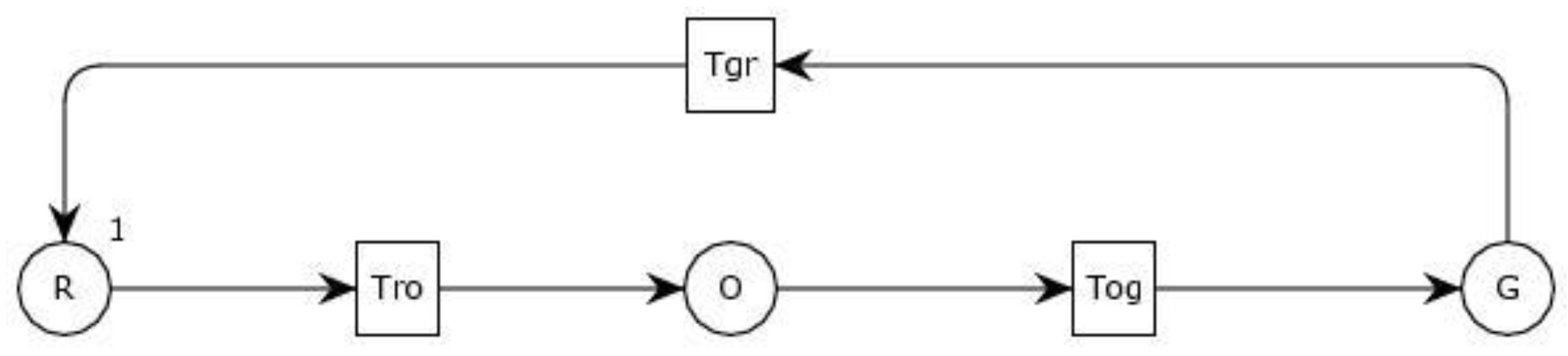
To understand a CPN, consider a simple traffic light signal. At any given instance, the traffic light can be in one of the three states: red, orange, or green. The signal changes its state after a fixed specified time. A Colored Petri Net model of this traffic light system is shown in Figure 1. The three states of the system, red, orange, and green are represented by places R, O, and G, respectively. The actions of going from state red to orange, from state orange to state green, and from state green to state red are represented by transitions Tro, Tog, and Tgr, respectively.

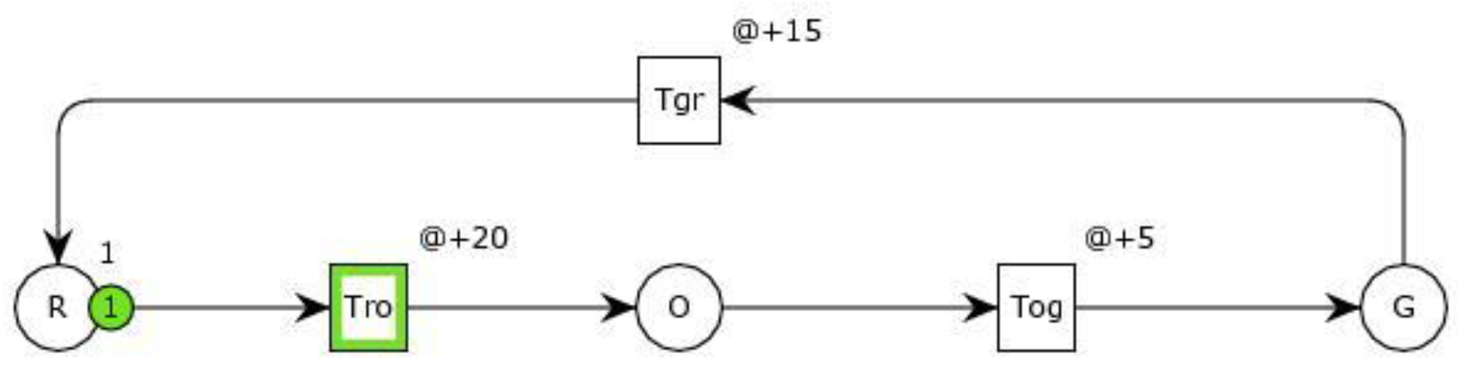
The temporal characteristics of the system are modeled with delays on the transitions. The value of 20 on transition Tro in Figure 2 suggests that after 20 time units the traffic light will be in the orange state. Similarly, the values of 5 and 15 on transitions Tog and Tgr reflect the time delays which the traffic light will experience to be in the green and the red state, respectively.

The presence of a single token at place R in Figure 2 shows that the traffic light is currently in the state red. In the absence of expressions on the input arcs of a transition and guard expression, a transition is said to be enabled and ready to fire when all the input places have at least a single token available in them. The firing of a transition signifies that the event represented by that transition has taken place. A transition, when fired, takes token(s) from its input place(s) and produces token(s) for the output place(s).

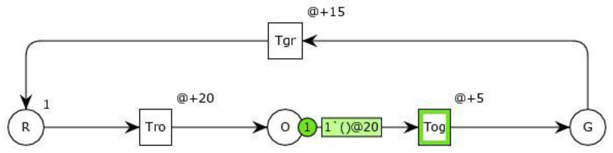
As seen in Figure 2, transition Tro is enabled and is ready to fire. Once it fires, it consumes the token from place R and produces a token for place O as shown in Figure 3. This suggests that the traffic light has changed its state from red to orange. The token at place O shows that the traffic light is now in the state orange and it has changed its state after 20 time units.

To verify if a particular property holds true in the complete state space of a model, the reachability graph of a CPN is analyzed. The nodes in the graph correspond to the reachable markings of the CPN model and its edges correspond to the transitions of the CPN model from one marking to another.

Table 1. Colored Petri Net Properties.

Property	Description
Boundedness	It ensures that a place does not contain more tokens then its defined capacity.
Terminating	It ensures that the model is terminating
Dead Transition	It ensures that all the functionality of the system being modeled is used in principle
Liveness	It ensures that a functionality of the modeled system can always be used again. It is mutually exclusive with the Terminating property

presents the fundamental properties of a CPN model that can be verified through reachability analysis along with a brief description [6].

The reachability analysis report of the traffic light signal CPN (Figure 2) is summarized in

Table 2. Reachability Analysis Report for the Traffic Light Signal.

Property	Result
Boundedness
Upper Bound	1
Lower Bound	0
Terminating
Dead Marking	None
Dead Transition	None
Liveness
Live Transitions	All

. The report was generated in CPNTools [3] which automatically analyzes the reachability graph of a CPN model. The values of 1 and 0 for the upper and lower bounds signify the maximum and the minimum number of tokens that each place will have. The absence of dead marking reflects that the traffic light system is a continuous and ongoing system. The lack of a dead transition ensures that all the features of a traffic light system are used and since all transitions are live it also ensures that all the functionalities can be used again.

2.2. Literature Review

Several algorithms have been proposed for solving the Multiple Traveling Salesman Problem. These solutions have been proposed from three different approaches, namely (1) exact solutions, (2) using heuristics, and (3) transformation to TSP.

An earlier work on presenting an exact solution to mTSP is that of Laporte and Nobert [7] whose solution is based on the relaxation of a few constraints of the original problem. Kara and Bektas [8] proposed an integer linear programming-based solution addressing sub-tour elimination constraints (SEC), whereas Kulkarni and Bhave [9] proposed different SECs to provide a solution to the Vehicle Routing Problem (VRP)—a special case of mTSP. A branch and bound algorithm is proposed by Ali and Kennington [10] that provides a solution to the asymmetric case of mTSP.

In large-scale problems where it is difficult to find an optimal solution, heuristic-based algorithms are used to provide a sub-optimal solution. The heuristic-based algorithms to solve the Multiple Traveling Salesman Problem include the Evolutionary Algorithm [11], Genetic Algorithm [12], Tabu Search [13], Simulated Annealing [14], and Neural Networks [15]. A hybrid approach that uses the Genetic Algorithm (GA) and the Gravitational Emulation Local Search (GELS) algorithm is proposed by Hosseinabadi et al. [16] that addresses the complex situations of mTSP.

Another approach to solving the Multiple Traveling Salesman Problem is to transform it into a simple Traveling Salesman Problem, solving the transformed problem with the available algorithms, thus addressing the original problem. The work presented by Hong and Padberg [17], Rao [18], and Jonker and Volgenant [19] proposes the transformation of symmetric mTSP to symmetric TSP whereas the transformation suggested by Bellmore and Hong [20] converts the asymmetric mTSP to an asymmetric TSP.

Colored Petri Nets have been used extensively in the modeling and analysis of systems from various domains. Wu [21] modeled manufacturing systems with CPN and analyze them to find the conditions required to avoid deadlock during its operation. Piera et al. [22] modeled a logistic and manufacturing system through CPN and performed simulation analysis to improve the system’s performance. Zaitsev [23] used CPN to model a switched Local Area Network and estimated its buffer size and response time through simulation. Aalst [24] suggested a transformation of scheduling problems to Timed Petri Nets and used analysis techniques to find conflicting and redundant scheduling precedence, and to put a lower and upper bound on the time required to finish tasks. A class of Petri Nets known as the Stochastic Petri Nets (SPNs) has been used to propose efficient scheduling mechanism for grid-based systems [25] and for optimizing the execution time for tasks in such systems [26].

3. Proposed Mapping

To transform a Multiple Traveling Salesman Problem (mTSP) onto the Colored Petri Net (CPN), the following mechanism is suggested to map the concepts of a city, a depo, a salesman and time from mTSP to the notations of place and transition from CPN.

By defining the Multiple Traveling Salesman Problem (mTSP) as a tuple {m, C, X, W}, where

• m = number of salesmen, and m > 1
• C = list of cities with C1, C2, C3, …, Cn
• X = starting point or depo
• W = cost matrix with Wij representing the time required to travel from city Ci to city Cj, for i,j = 1,2,3, …, n

and with the following assumptions

• All salesmen start their tour from depot X
• The salesmen are not required to return to the depo after visiting the cities

the concepts of city, depo, salesman, and time are mapped onto the places and transitions as follows

3.1. Mapping City

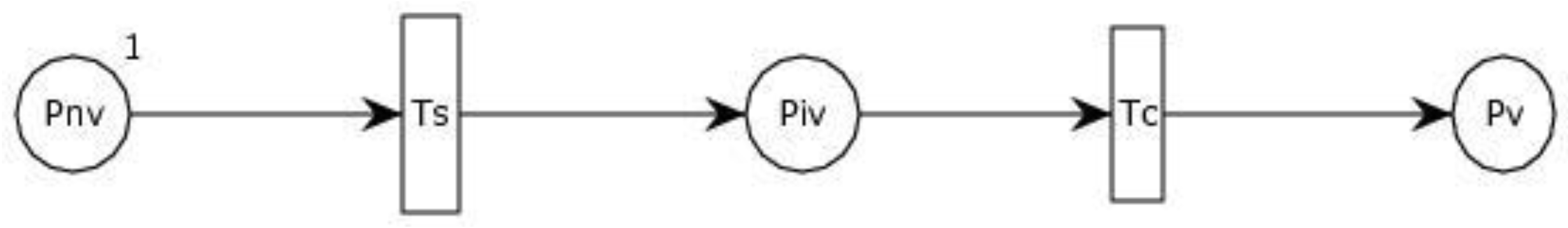
A city C can have three possible states: (1) not yet visited, (2) being visited, and (3) visited. For these three states, two events are identified: (1) when a salesman arrives at the city C and (2) when the salesman departs from the city. These three states and two events are mapped onto the places and the transitions as shown in Figure 4. The places Pnv, Piv, and Pv corresponds to the states of a city whereas the transitions Ts and Tc correspond to the arrival and the departure of the salesman, respectively. Initially, the place Pnv contains a single token which means that the city has not yet been visited.

3.2. Mapping Depo and Number of Salesman

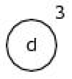
The place, X, from which a salesman starts its tour—also knowns as the depo—is modeled with a single place d as shown in Figure 5. The place d is connected to the place Pnv through the transition Ts for each city that has a route defined from the depo to that city. The number of salesman, m, is modeled through the initial marking on the place d. In Figure 5, the number of tokens at place d is 3, which means that the number of salesmen is three.

3.3. Mapping Time and Routes between Cities

The route from one city to the other city is mapped by connecting the place Pv of the first city with the place Piv of the second city through a transition T. The time to reach any city from depo X is mapped by the inscription on the arc connecting the transition Ts and the Piv of that city, whereas, the time required to go from one city to the other is mapped by writing an inscription on the arc connecting the transition T with the place Piv of the destination city.

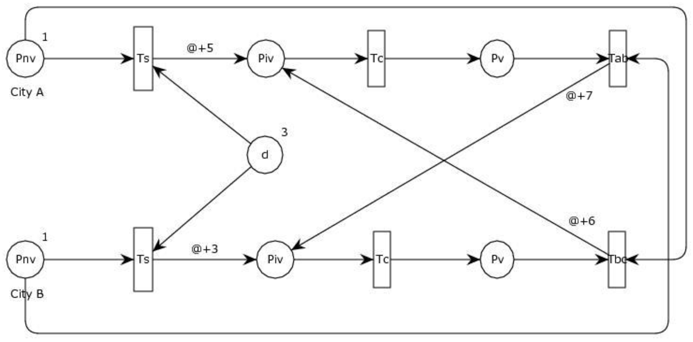
As shown in Figure 6, the place Pv of City A is connected to the place Piv of City B through the transition Tab. This suggests that a route for the salesman is available from City A to City B. The inscription 5 on the arc, connecting the transition Ts with the place Piv of City A, illustrates the time a salesman would take to reach City A from the depo X. Similarly, the inscription of 7 on the arc connecting the transition Tab with the place Piv of City B illustrate the time a salesman would take to reach City B from City A.

A flowchart of the proposed algorithm is shown in Figure 7 while the complete mapping of various mTSP concepts to CPN constructs is formally presented in

Table 3. Algorithm to map mTSP onto CPN.

Steps	Description
Step 1	Create place d with an initial marking m.
Step 2 a	For each city create three places: Pnv, Piv and Pv.
Step 2 b	Set initial marking for each Pnv as 1.
Step 2 c	For each city C, connect places Pnv and Piv through transition Ts and places Piv and Pv through transition Tc.
Step 3 a	For each route defined from depo X to a city C, connect place d and place Piv of the city C through transition Ts.
Step 3 b	Place an inscription on the arc connecting the transition Ts and the place Piv equals to the time taken to go from the depo to the city.
Step 4 a	For each route defined from City(i) to City(j), connect the place Pv(i) and Piv(j) through transition Tij.
Step 4 b	Place an inscription on the arc connecting Transition Tij and the place Piv(j) equal to the time required to go from City(i) to City(j).
Step 4 c	Connect place Pnv(j) and transition Tij with an arc

. The algorithm presented in Table 3 can transform any given mTSP into a CPN.

4. Case Study

To explain the working of the algorithm, presented in Table 3, three different cases are presented in this section. The first two cases address the Multiple Traveling Salesman Problem (mTSP), whereas the third and the last case address the Traveling Salesman Problem (TSP)—a special case of the Multiple Traveling Salesman Problem. The mTSP involves five cities and three salesmen, whereas the TSP involves three cities and a single salesman. The transformed CPN model from each case is simulated in CPNTools [26], an open-source tool to create, simulate and analyze Colored Petri Nets. Two optimization objectives are evaluated for the case studies: (a) minimizing the sum of traveling time over all salesmen (miniSUM) and (b) minimizing the maximum time of a single salesman over all salesmen (miniMAX) [27].

4.1. Case One: mTSP with Symmetric Cost Matrix

In the first case all cities are connected to each other and the time to move from city A to city B is same as the time to move from city B to city A. The cost matrix used in this case is shown in

Table 4. Symmetric Cost Matrix for mTSP with five cities.

	X	A	B	C	D	E
X	0	1	2	3	4	5
A	1	0	6	7	8	9
B	2	6	0	2	3	4
C	3	7	2	0	7	8
D	4	8	3	7	0	3
E	5	9	4	8	3	0

.

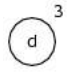
In the first step, the depo and the number of salesmen are transformed as shown in Figure 8.

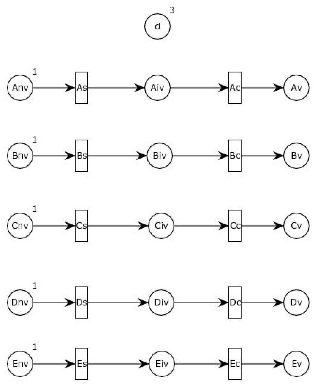
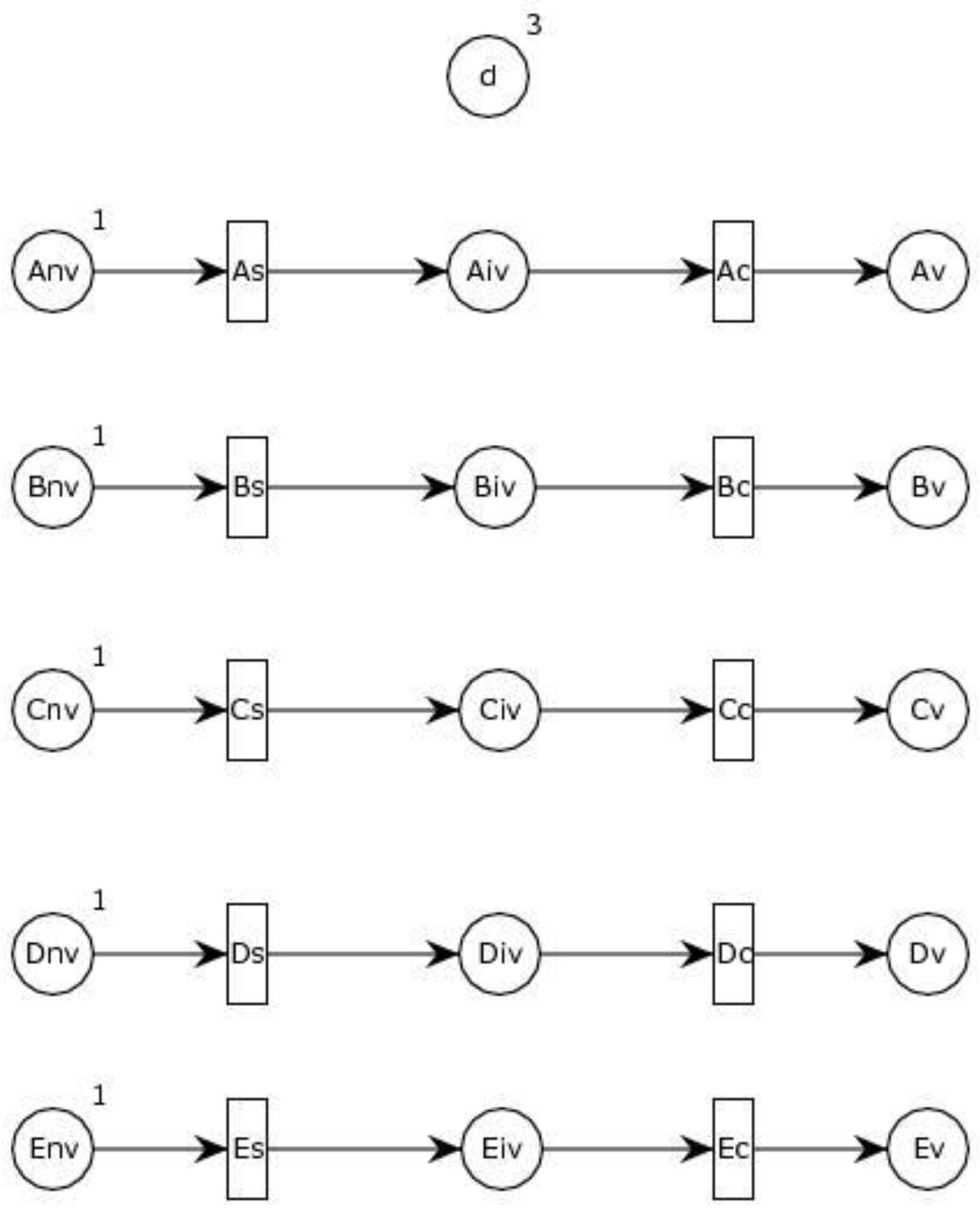
In the second step, five cities are transformed as shown in Figure 9.

In the third step, the routes between the depo and the cities along with the time are transformed as shown in Figure 10.

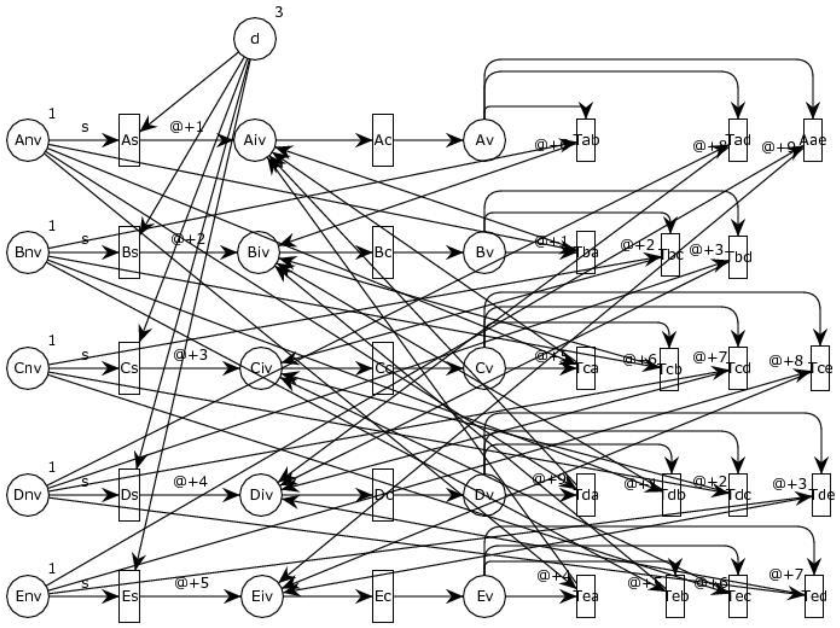
Finally, in the last step, the routes between the cities, along with the time, are transformed as shown in Figure 11.

4.2. Case B: mTSP with Asymmetric Cost Matrix

The second case is similar to the previous case regarding the complete connectivity between the cities but this case assumes that the cost of going from the first city to the second is not necessarily same as the cost of going from the second city to the first. It can be seen from the cost matrix shown in

Table 5. Asymmetric cost matrix for mTSP with five cities.

	X	A	B	C	D	E
X	0	1	2	3	4	5
A	1	0	6	7	8	9
B	2	1	0	2	3	4
C	3	5	6	0	7	8
D	4	9	1	2	0	3
E	5	4	5	6	7	0

that the cost of going from city A to city D is 8 units but the cost of going from city D to the city A is 9 units.

As was the case in the previous scenario, the first step is to create the depo and the number of salesmen as shown in Figure 12.

In the second step, the five cities are transformed as shown in Figure 13.

In the third step, the routes between the depo and the cities along with the time are transformed as shown in Figure 14.

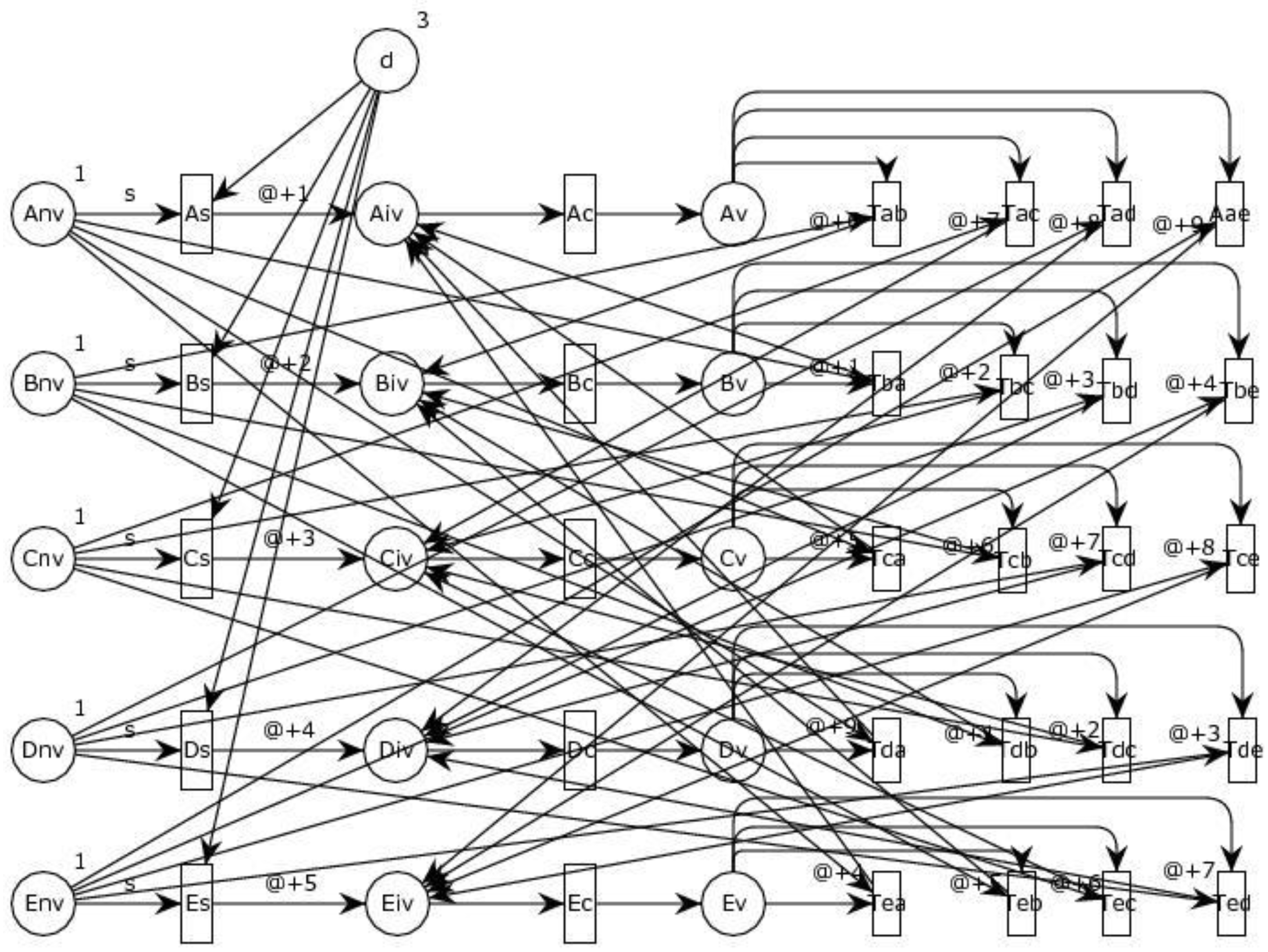
In the final step, only the routes that exist between the cities along with the time are transformed as shown in Figure 15. Since there is no direct route from city A to city C, or from city B to city E, the respective transitions Tac and Tbe are not created.

4.3. Case C: TSP with Symmetric Cost Matrix

In the third and final case, it is assumed that the cost matrix is symmetric and only one salesman is involved. This is a special case of mTSP in which m = 1 and is also known as a Traveling Salesman Problem. The cost matrix for this case is presented in

Table 6. Symmetric cost matrix for three cities.

	X	A	B	C
X	0	7	13	5
A	7	0	4	6
B	13	4	0	9
C	5	6	9	0

and the transformed model based on the algorithm from Table 1 is shown in Figure 16.

4.4. Simulation Results

The transformed CPN models of all three cases are simulated in CPNTools and the results are summarized in

Table 7. Simulation Results.

Optimization Objective	Case A (Time Units)	Case B (Time Units)	Case C (Time Units)
miniSUM	18	18	NA
miniMAX	8	7	15

. The table presents the simulation results for the two optimization objectives, namely, the miniSUM and the miniMAX.

The simulation was run ten times for each of the three cases. The minimum sum of time over the three salesmen (miniSUM) achieved both with symmetric cost matrix in case A and with asymmetric cost matrix in case B is 18 time units. The minimum of the maximum time of a single salesman over the three salesmen (miniMAX) achieved with symmetric cost matrix (case A) is 8 time units and it is 7 time units when the cost matrix is asymmetric (case B).

In case C, where there is only a single salesman, the objective function of the minimum sum of time over all the salesmen (miniSUM) is not applicable. For the objective function of the minimum of a maximum time of a single salesman over the three salesmen (miniMAX), the value achieved is 15 time units.

It must be noted that during a simulation in CPNTools, when there are more than one enabled transitions, each enabled transition is assigned an equal probability of being fired. Hence, the solution, which is generated after each simulation run, is a random solution from all the possible solutions. CPNTools do provide the tools to collect data from the simulation which can be used for statistical studies and calculating different performance related measures.

4.5. Reachability Analysis

The reachability graphs, which represent the state space of CPN models, are analyzed in this section to verify various properties. For the transformed mTSP model into CPN, the property of interest is the liveness property. Under the liveness property, the absence of dead transitions signifies that all the functionality that is being modeled is used while the presence of dead markings signifies that the model is not stuck in an infinite sequence of steps and terminates after a finite sequence of steps.

CPNTools provide support to automatically generate and analyze the reachability graph of the CPN model.

Table 8. Part of State Space Report.

	Liveness Properties
	Dead Transition Instances	Dead Markings
Case One	None	Present
Case Two	None	Present
Case Three	None	Present

presents a part of the state space report generated by CPNTools for all the three transformed models of mTSP. It can be seen that, in all the three cases, there are no dead transitions and there are dead markings under the liveness property. This verfies that all the cities are visited by the salesmen and the tour lengths are finite.

5. Comparison with Other Approaches

A qualitative comparison of the proposed algorithm with other approaches discussed earlier is summarized in

Table 9. Qualitative Comparison of the Proposed Algorithm with Other Approaches.

1 B = Both Symmetric and Asymmetric Cost Matrix, S = Symmetric Cost Matrix Only
2 Y = Yes, N = No
Approaches		Criterion A 1	Criterion B 2
Proposed Algorithm		B	Y
Exact Solutions	Laporte et al. [7]	B	Y
	Kara et al. [8]	B	Y
	Iqbal Ali et al. [10]	B	Y
Heuristics	Carter et al. [12]	S	N
	Song et al. [14]	B	N
	Wacholder et al. [15]	B	Y
	Hosseinabadi [16]	S	N
Transformation	Hong et al. [17]	S	Y
	Rao [18]	S	Y
	Jonker et al. [19]	S	Y

. The parameters used for evaluation are (a) type of cost matrix, and (b) ability to address the TSP—the special case of mTSP.

It can be seen from Table 9, for the evaluation parameter A—the type of cost matrix, the existing approaches do address both the symmetric and the asymmetric nature of the cost matrix. It can be concluded that if a solution could solve an asymmetric mTSP, then it can also be used to solve the symmetric mTSP.

For the evaluation parameter B—the ability to address TSP, both the exact based solutions and the transformations could also solve the TSP as it is a specific case of mTSP. However, the heuristics-based solutions, in general, and GA-based solutions, in particular, would require a different representation of chromosome for solving the TSP.

The proposed algorithm provides a feasible solution to the mTSP with either asymmetric or symmetric cost matrix. The proposed algorithm can also be used to transform and solve the Traveling Salesman Problem, which is a specific instance of mTSP. It must be noted that the real utility of the proposed mapping schemes comes into play as constraints are added to mTSP and finding even a feasible solution becomes a complicated task.

6. Conclusion and Future Direction

This paper presented an algorithm to transform a given asymmetric Multiple Traveling Salesman Problem onto Colored Petri Nets. The transformed model in CPN guarantees a feasible solution to the original mTSP problem. This paper also discusses the mechanism for mapping different concepts of depo, city, salesman, and time from mTSP onto the constructs of place and transition in CPN.

The mapped CPN models were simulated in CPNTools which is an open-source tool for creating, analyzing and simulating CPN models. The simulation results obtained were used to measure the minimum sum of traveling time over all the salesmen and the minimum time taken by a single salesman over all the salesmen. The proposed mapping has a limitation that as the number of cities increase, the corresponding transformation and modeling in CPN will get laborious and time consuming. To verify that the transformed model is correct and terminating, the reachability analysis of the model was performed in CPNTools which verified that the desired properties hold true.

In the future, the presented work will be extended to address other types of cost matrix incorporating distance, effort, and fuel. Efforts will also be made to solve variations of the mTSP with additional constraints. In addition, the simulation results will be used to measure other optimization objective functions, like minimizing the number of salesmen or maximizing the number of cities being visited. A comparison with other optimization techniques will also form part of our future research.

References

- Bektas, T. The multiple traveling salesman problem: An overview of formulations and solution procedures. Omega 2006, 34, 209–219. [Google Scholar] [CrossRef]
- Hoffman, K.L.; Padberg, M.; Rinaldi, G. Traveling Salesman Problem. In Encyclopedia of Operations Research and Management Science; Gass, S.I., Fu, M.C., Eds.; Springer: Boston, MA, USA, 2013; pp. 1573–1578. [Google Scholar] [Green Version]
- Ratzer, A.V.; Wells, L.; Lassen, H.M.; Laursen, M.; Qvortrup, J.F.; Stissing, M.S.; Westergaard, M.; Christensen, S.; Jensen, K. CPN Tools for Editing, Simulating, and Analysing Coloured Petri Nets. In Applications and Theory of Petri Nets 2003; van der Aalst, W.M.P., Best, E., Eds.; Springer: Berlin, Germany, 2003; pp. 450–462. [Google Scholar]
- Jensen, K. Coloured petri nets: A high level language for system design and analysis. In Advances in Petri Nets 1990; Springer: Berlin, Heidelberg, 1989; pp. 342–416. [Google Scholar]
- Petri, C.A. Kommunikation mit Automation. Diss. Univ. Bonn 1962, 2, 128. [Google Scholar]
- Jensen, K.; Kristensen, L.M. Coloured Petri Nets: Modelling and Validation of Concurrent Systems, 1st ed.; Springer: Berlin, Germany, 2009. [Google Scholar]
- Laporte, G.; Nobert, Y. A Cutting Planes Algorithm for the m-Salesmen Problem. J. Oper. Res. Soc. 1980, 31, 1017–1023. [Google Scholar] [CrossRef]
- Kara, I.; Bektas, T. Integer linear programming formulations of multiple salesman problems and its variations. Eur. J. Oper. Res. 2006, 174, 1449–1458. [Google Scholar] [CrossRef]
- Kulkarni, R.V.; Bhave, P.R. Integer programming formulations of vehicle routing problems. Eur. J. Oper. Res. 1985, 20, 58–67. [Google Scholar] [CrossRef]
- Iqbal Ali, A.; Kennington, J.L. The asymmetric M-travelling salesmen problem: A duality based branch-and-bound algorithm. Discrete Appl. Math. 1986, 13, 259–276. [Google Scholar] [CrossRef]
- Fogel, D.B. A parallel processing approach to a multiple traveling salesman problem using evolutionary programming. In Proceedings of the fourth annual symposium on parallel processing, Fullerton, CA, USA, April 1990; pp. 318–326. [Google Scholar]
- Carter, A.E.; Ragsdale, C.T. A new approach to solving the multiple traveling salesperson problem using genetic algorithms. Eur. J. Oper. Res. 2006, 175, 246–257. [Google Scholar] [CrossRef]
- Cordeau, J.-F.; Gendreau, M.; Laporte, G. A tabu search heuristic for periodic and multi-depot vehicle routing problems. Networks 1997, 30, 105–119. [Google Scholar] [CrossRef]
- Song, C.-H.; Lee, K.; Lee, W.D. Extended simulated annealing for augmented TSP and multi-salesmen TSP. In Proceedings of the 2003 International Joint Conference on Neural Networks, Portland, OR, USA, 20–24 July 2003; pp. 2340–2343. [Google Scholar]
- Wacholder, E.; Han, J.; Mann, R.C. A neural network algorithm for the multiple traveling salesmen problem. Biol. Cybern. 1989, 61, 11–19. [Google Scholar] [CrossRef]
- Hosseinabadi, A.A.R.; Kardgar, M.; Shojafar, M.; Shamshirband, S.; Abraham, A. GELS-GA: Hybrid metaheuristic algorithm for solving Multiple Travelling Salesman Problem. In Proceedings of the 14th International Conference on Intelligent Systems Design and Applications, Okinawa, Japan, 27–29 November 2014; pp. 76–81. [Google Scholar]
- Hong, S.; Padberg, M.W. Technical Note—A Note on the Symmetric Multiple Traveling Salesman Problem with Fixed Charges. Oper. Res. 1977, 25, 871–874. [Google Scholar] [CrossRef] [Green Version]
- Rao, M.R. Technical Note—A Note on the Multiple Traveling Salesmen Problem. Oper. Res. 1980, 28, 628–632. [Google Scholar] [CrossRef] [Green Version]
- Jonker, R.; Volgenant, T. Technical Note—An Improved Transformation of the Symmetric Multiple Traveling Salesman Problem. Oper. Res. 1988, 36, 163–167. [Google Scholar] [CrossRef] [Green Version]
- Bellmore, M.; Hong, S. Transformation of Multisalesman Problem to the Standard Traveling Salesman Problem. J. ACM 1974, 21, 500–504. [Google Scholar] [CrossRef]
- Wu, N. Necessary and sufficient conditions for deadlock-free operation in flexible manufacturing systems using a colored Petri net model. IEEE Trans. Syst. Man Cybern. Part C Appl. Rev. 1999, 29, 192–204. [Google Scholar]
- Piera, M.À.; Narciso, M.; Guasch, A.; Riera, D. Optimization of Logistic and Manufacturing Systems through Simulation: A Colored Petri Net-Based Methodology. Simulation 2004, 80, 121–129. [Google Scholar] [CrossRef]
- Zaitsev, D.A. Switched LAN simulation by colored Petri nets. Math. Comput. Simul. 2004, 65, 245–249. [Google Scholar] [CrossRef]
- van der Aalst, W.M.P. Petri net based scheduling. Oper. Res. Spektrum 1996, 18, 219–229. [Google Scholar] [CrossRef] [Green Version]
- Shojafar, M.; Pooranian, Z.; Abawajy, J.H.; Meybodi, M.R. An efficient scheduling method for grid systems based on a hierarchical stochastic petri net. J. Comput. Sci. Eng. 2013, 7, 44–52. [Google Scholar] [CrossRef]
- Shojafar, M.; Pooranian, Z.; Meybodi, M.R.; Singhal, M. ALATO: An efficient intelligent algorithm for time optimization in an economic grid based on adaptive stochastic Petri net. J. Intell. Manuf. 2015, 26, 641–658. [Google Scholar] [CrossRef]
- Gini, M. Multi-robot allocation of tasks with temporal and ordering constraints. In Proceedings of the 31st AAAI Conference on Artificial Intelligence, AAAI 2017, San Francisco, CA, USA, 4–10 February 2017; pp. 4863–4869. [Google Scholar]
Figure 1.
CPN Model of a Traffic Light System.
Figure 2.
CPN Model of a Traffic Light System with Temporal Behavior.
Figure 3.
CPN Model of Traffic Light after Firing of Transition Tro.
Figure 4.
CPN Model of a City.
Figure 5.
CPN model of a depo, two cities and three salesmen.
Figure 6.
CPN model of a Multiple Traveling Salesman Problem.
Figure 7.
Flowchart of the Proposed Algorithm.
Figure 8.
Depo with three salesmen.
Figure 9.
Depo with three salesmen and five cities.
Figure 10.
Five cities connected through depo.
Figure 11.
mTSP involving five connected cities, a depo and three salesmen with symmetric cost matrix.
Figure 12.
Figure 13.
Figure 14.
Figure 15.
mTSP involving five connected cities, a depo and three salesmen with asymmetric cost matrix.
Figure 16.
TSP involving three cities with symmetric cost matrix.