A Simplified Matrix Formulation for Sensitivity Analysis of Hidden Markov Models

1
Department of Electrical and Computer Engineering, North Carolina A&T State University, Greensboro, NC 27411, USA
2
Department of Computer Science, North Carolina A&T State University, Greensboro, NC 27411, USA
*
Author to whom correspondence should be addressed.
Algorithms 2017, 10(3), 97; https://doi.org/10.3390/a10030097
Submission received: 9 June 2017
/
Revised: 6 August 2017
/
Accepted: 14 August 2017
/
Published: 22 August 2017
Abstract
:In this paper, a new algorithm for sensitivity analysis of discrete hidden Markov models (HMMs) is proposed. Sensitivity analysis is a general technique for investigating the robustness of the output of a system model. Sensitivity analysis of probabilistic networks has recently been studied extensively. This has resulted in the development of mathematical relations between a parameter and an output probability of interest and also methods for establishing the effects of parameter variations on decisions. Sensitivity analysis in HMMs has usually been performed by taking small perturbations in parameter values and re-computing the output probability of interest. As recent studies show, the sensitivity analysis of an HMM can be performed using a functional relationship that describes how an output probability varies as the network’s parameters of interest change. To derive this sensitivity function, existing Bayesian network algorithms have been employed for HMMs. These algorithms are computationally inefficient as the length of the observation sequence and the number of parameters increases. In this study, a simplified efficient matrix-based algorithm for computing the coefficients of the sensitivity function for all hidden states and all time steps is proposed and an example is presented.
1. Introduction
A Hidden Markov Model (HMM) is a stochastic model of the dynamic process of two related random processes that evolve over time. A set of stochastic processes that produces the sequence of observed symbols is used to infer an underlying stochastic process that is not observable (hidden states). HMMs have been widely utilized in many application areas including speech recognition [1], bioinformatics [2], finance [3], computer vision [4], and driver behavior modeling [5,6]. A comprehensive survey on the applications of HMMs is presented in [7]. A simple dynamic Bayesian network can be used to represent a stationary HMM with discrete variables [8,9]. Consequently, algorithms and theoretical results developed for dynamic Bayesian networks can be applied to HMMs as well.
Sensitivity analysis in HMMs has been done by perturbation analysis in which a brute-force computation of the effect of small changes on the output probability of interest is done [10,11]. Sensitivity analysis research has shown that a functional relationship can be established between a parameter variation and the output probability of interest. This function can represent the effect of any change in the parameter under consideration as compared to the perturbation analysis. Consequently, the goal of sensitivity analysis becomes developing techniques to create this function. This general function will also enable us to compute bounds on the output probabilities without sensitivity analysis [12,13,14,15].
The objective of this work is to develop an algorithm for sensitivity analysis in HMMs directly from the model’s representation. Our focus is on parameter sensitivity analysis where the variation of the output is studied as the model parameters vary. In this case, the parameters are the (conditional) probabilities of the HMM model (initial, transition, and observation parameters) and the output is some posterior probability of interest (filtering, smoothing, predicted future observations, and most probable path).
Parametric sensitivity analysis can be used for multiple purposes. The sensitivity analysis can be used to identify those parameters which have significant impact on the output probability of interest. Consequently, the result can be used as a basis for parameter tuning and studying the robustness of the model output to changes in the parameters [16,17,18].
Many researchers study the problem of sensitivity analysis in Bayesian Networks and HMMs. There are two approaches used to compute the constants of the sensitivity function in the standard Bayesian network inference algorithms. The first method is solving systems of linear equations [19] by evaluating the sensitivity function for different values of the varying parameter . The second is based on a differential approach [20] by which the coefficients of a multivariate sensitivity function can be computed from partial derivatives. The tailored version of the junction tree algorithm has been used to establish the sensitivity functions in Bayesian networks more efficiently [21,22]. In [23], sensitivity analysis of Bayesian networks for multiple parameter changes is presented. In [24], credal sets that are known to represent the probabilities of interest are used for sensitivity analysis of Markov chains. In [10,11], sensitivity analysis of HMMs based on small perturbations in the parameter values is presented. A tight perturbation bound is derived and it is shown that the distribution of the HMM tends to be more sensitive to perturbations in the emission probabilities than to the transition and initial distributions. A tailored approach for HMM sensitivity analysis, the Coefficient-Matrix-Fill procedure, is presented in [25,26]. It directly utilizes the recursive probability expressions in an HMM. Consequently, it improves the computational complexity of applying the existing approaches for sensitivity analysis in Bayesian networks to HMMs. In [27], imprecise HMMs are presented as a tool for performing sensitivity analysis of HMMs.
In this paper, we propose a sensitivity analysis algorithm for HMMs using a simplified matrix formulation directly from the model representation based on a recently proposed technique called the Coefficient-Matrix-Fill procedure [26]. Until recently, sensitivity analysis in HMMs has been performed using Bayesian network sensitivity analysis techniques. The HMM is represented as a dynamic Bayesian network unrolled for a fixed number of time slices, and the Bayesian sensitivity algorithms are used. However, these algorithms do not utilize the HMMs’ recursive probability formulations. In this work, a simple algorithm based on a simplified matrix formulation is proposed. In this algorithm, to calculate the coefficients of the sensitivity functions, a series of Forward matrices are used, where k represents the time slice in the observation sequence. The matrices (Initial, Transition, and Observation) where the corresponding model parameter varies are decomposed into the parts independent of and dependent on for mathematical convenience. This enables us to compute the coefficients of the sensitivity function at each iteration in the recursive probability expression and implement the algorithm in a computer program. These matrices are computed based on a proportional co-variation assumption. The Observation Matrix O is represented as diagonal matrices whose vth diagonal entry is for each state v and whose other entries are 0 at the time t of the observation sequence. The proposed algorithm is computationally efficient as the length of the observation sequence increases. It computes the coefficients of a polynomial sensitivity function by filling coefficient matrices for all hidden states and all time steps.
The paper is organized as follows. In Section 2, the background on HMM and Sensitivity Analysis in HMM is presented. The details of the proposed algorithm for the filtering probability sensitivity function are explained in Section 3. In Section 4, the sensitivity analysis of the smoothing probability using the proposed algorithm is discussed. Finally, the paper is concluded with a summary of the results achieved and recommendations for future research works.
2. Background
In this section, we present the background on HMMs and Sensitivity Analysis in HMMs. First, we will discuss HMMs, HMM inference tasks and their corresponding recursive probability expressions. Then sensitivity analysis in HMMs is explained based on the assumption of proportional co-variation, and a univariate polynomial sensitivity function whose coefficients the proposed algorithm computes is defined. Here, the variables are denoted by capital letters and their values by lower case letters.
2.1. Hidden Markov Models
An HMM is a stochastic statistical model of a discrete Markov chain of a finite number of hidden variables X that can be observed by a sequence of a set of output variables Y from a sensor or other sources. The probability of transitioning from one state to another in this Markov chain is time-invariant, which makes the model stationary. The observed variables Y are stochastic with the observation (emission) probabilities, which are also time invariant. The overall HMM consists of n distinct hidden states of the Markov chain and m corresponding observable symbols. In general, the observations can be discrete or continuous, however, in this work, we focus on the discrete observations. The variable X has hidden states, denoted by , and the variable Y has observable symbols, denoted by . Formally, an HMM is specified by a set of parameters that are defined as follows:
- The prior probability distribution (initial vector) has entries , which are the probabilities of state being the first state in the Markov chain.
- The transition matrix A has entries , which are the probabilities of transit from state to state in the Markov chain.
- The observation matrix O has entries , which are the probabilities to observe if the current state is .
An example of an HMM where X has two states and Y three symbols is shown in Figure 1a. The two states are and and based on them three symbols , or are observed. The parameters of the HMM (including initial vector, transition matrix and observation matrix) are also shown in Figure 1a.
The dynamic Bayesian network representation of the HMM in Figure 1a is shown in Figure 1b, unrolled for T time slices [8,9]. The initial vector, transition matrix and observation matrix of the HMM are represented by the labels , A and O respectively, attached to the nodes in the Bayesian network graph. The superscript for the variables X and Y and their values indicate the time slice under consideration.
In this paper, denotes the actual evidence for the variable Y in time slice t and represents a sequence of observations where is a sequence of observations from the set . The representation denotes the actual state , for the variable X in time slice t.
2.1.1. Inference in HMMs
In temporal models, inference means computing the conditional probability distribution of X at time t, given the evidence up to and including time T, that is . The main inference tasks include filtering for , prediction of a future state for and smoothing, that, is inferring the past for . In an HMM, the Forward-Backward algorithms are used for the inference tasks and training of the model using an iterative procedure called the Baum-Welch method (Expectation Maximization) [28,29,30]. The Forward-Backward algorithms computes the following probabilities for all hidden states i at time :
- forward probability , and
- backward probability
resulting in
For , the algorithm can be applied by taking and adopting the convention that the configuration of an empty set of observations is TRUE, i.e., , giving
As shown in Equation (1), any conditional probability can be calculated from the joint probabilities for all hidden states i using Bayes’ theorem. Since our objective is sensitivity analysis of the HMM output probability of interest for parameter variations, in the remainder of this paper our focus will be on the joint probabilities for all hidden states i.
The other important inference tasks are the prediction of future observations, i.e., for , finding the most probable explanation, i.e., using the Viterbi Algorithm and learning the HMM parameters as new observations come in using the Baum-Welch algorithm, which can be achieved by the Forward-Backward algorithms. The prediction of future observations can be computed as the fraction of the two probabilities , , and , which are computed using forward probabilities.
Note that if , then can be computed by setting all in-between observations , , to as above.
2.1.2. Recursive Probability Expressions
In order to establish the sensitivity functions for HMMs directly from the model’s representation, the recursive probability expression for the Forward-Backward algorithm should be investigated. The repetitive character of the model parameters in the Forward-Backward algorithm is used to drive the sensitivity functions. Consequently, in this section the recursive expressions of the Forward-Backward algorithm [29,31] are reviewed briefly.
Filtering. The filter probability is for a specific state v of X. This probability is the same as the forward probability in the Forward-Backward algorithm. For time slice , we simply have that
where corresponds to the symbol of Y that is observed at time 1. For time slices , we exploit the fact that is independent of , given , written . Then,
The first factor in the above product corresponds to ; conditioning the second factor on the n states of , we find with that
Taken together, we find for the recursive expression
Prediction. The prediction probability for can be handled by the the Forward-Backward algorithm by computing with an empty set of evidence for . It can be implemented by replacing the term by 1 for in Equation (2). As a result, for , the prediction probability becomes the prior probability . The prediction task can be seen as a special case of the filtering task.
Smoothing. Finally, we consider a smoothing probability with . Using we find that
The second term in this product is a filter probability; the first term is the same as the backward probability in the Forward-Backward algorithm. By conditioning the first term on and exploiting the independences and for , we find that
For , this results in
Taken together, we find for the recursive expression
In this work, we present the sensitivity of the HMM for filtering and smoothing probabilities for transition, initial and observation parameter variation. Therefore, the above discussion on the recursive probability expression for the filtering probability, Equation (2), and smoothing probability Equation (3), will be used to formulate our algorithm.
2.2. Sensitivity Analysis in HMM
As shown in recent studies [13,25,32,33], sensitivity analysis is establishing a functional relationship that describes how output probability varies as the network’s parameters change. A posterior marginal probabilities, , where v is value of a variable V and e is the evidence available, is considered to represent the output probabilities of interest. The network parameter under consideration is represented as for a value of a variable V, and is an arbitrary combination of the values of the set of evidences of V. So represents the posterior marginal probabilities as a function of .
Consequently, when the parameter varies, each of the other conditional probabilities from the same distribution co-vary accordingly by the ratio between the the remaining probabilities. That is, if a parameter for a variable V is varied, then
The co-variation simplifies to for binary-valued V. The sensitivity function is defined based on the stated proportional co-variation assumption. The constants in the general form of the sensitivity function are generated from the network’s parameters that are neither varied nor co-varied, and their values depend on the output probability of interest. A sensitivity function for a posterior probability of interest is a quotient of two polynomial functions, since , and hence a rational function.
We have the following univariate polynomial sensitivity function to define the joint probability of a hidden state and a sequence of observations as a function of a model parameter .
3. Sensitivity Analysis of Filtering Probability
In this section, the simplified matrix formulation for sensitivity of the filtering probability to the variation of the initial, transition and observation parameters is proposed. Let us consider the sensitivity functions for a filtering probability and the variation of one of the model parameters, viz., . From Equation (2), the forward recursive filtering probability expression, it follows that
where
and
The sensitivity function coefficients are computed by the proposed method using a series of Forward matrices . The sensitivity of the filtering probability for transition, initial and observation parameter variations is formulated in the next subsections.
3.1. Transition Parameter Variation
In this subsection, the simplified matrix formulation (SMF) for sensitivity of the filtering probability to variation of the transition parameter is proposed. Let us consider the sensitivity functions for a filtering probability and transition parameter . From Equation (6), the recursive filtering probability sensitivity function, it follows that for we have the constant , and for ,
In the next sub-subsections, the formulation of the proposed method to compute the coefficients of the sensitivity function in Equation (5) is presented in detail. First, the decomposition of the transition matrix into the parts of A independent of and dependent on and the observation matrix representation for the simplified matrix formulation is presented. Then the SMF representation for the sensitivity of the filtering probability to transition parameter variation and its algorithm implementation are discussed.
3.1.1. Transition Matrix Decomposition and Observation Matrix Representation
In the proposed algorithm, to calculate the coefficients in a series of Forward matrices , the Transition Matrix A is divided into and that are independent of and dependent on , respectively, for mathematical convenience. The matrices and are computed based on the proportional co-variation assumption shown in Equation (4). Let us explain the decomposition considering an HMM with an Transition Matrix A with the transition parameter . This makes the transition matrix A a function of , and, with the proportional co-variation assumption shown in Equation (4), it becomes
This matrix is divided into and that are independent of and dependent on , respectively, as follows, and such that = + .
In short, this decomposition can be represented in the algorithm simply as and that are independent of and dependent on , respectively.
In the simplified matrix representation, the Observation Matrix O is represented as an diagonal matrices whose diagonal entry is for each state v and whose other entries are 0 at the time t of the observation sequence [31]. Let us explain this representation by considering the HMM with an Observation Matrix O. Given the following sequence of observations: and , the corresponding diagonal matrices become
3.1.2. SMF for Sensitivity Analysis of the Filtering Probability to the Transition Parameter Variation
In the Simplified Matrix Representation (SMF), the sensitivity function shown in Equation (7) can be written as a simple matrix-vector multiplication. It follows that for we have the constant , which becomes in the SMF. For , we have
which is represented in SMF as
The overall procedure of computing the sensitivity coefficients of using the SMF is described in the following algorithm.
3.1.3. Algorithm Implementation
This algorithm summarizes the proposed technique, where e is the sequence of observations and , and solves the recursive Equation (7). Once the Transition and Observation matrices are represented in SMF as explained above, the sensitivity coefficients are computed by filling the forward matrices for . The details of filling contents of the forward matrices in Algorithm 1 are explained as follows. is initialized by the matrix multiplications of , which is a diagonal matrix whose diagonal entry is , and the initial distribution vector ,
The remaining matrices of size are initialized by filling them with zeros. Two temporary matrices and are used for computing the coefficients as explained previously. is computed as the matrix multiplication of , (which is independent of ) and , and a zero vector of size n (= the number of states) is appended at its end. represents the recursion in the filtering probability. In the same way is computed as the matrix multiplication of , (which is dependent on ) and , and a zero vector of size n is appended to the front. Then is set as the sum of and :
| Algorithm 1 Computes the coefficients of the forward (filtering) probability sensitivity function with in forward matrices for using SMF. |
| Input: |
| Output: |
|
3.2. Initial Parameter Variation
In this subsection, the sensitivity of the filtering probability to the initial parameter variation is derived based on SMF. Let us consider the sensitivity functions for a filtering probability and variation in the initial parameter . From Equation (6), the recursive filtering probability sensitivity expression, for , we have , and for ,
3.2.1. Initial Vector Decomposition
In the proposed algorithm, to calculate the coefficients in a series of forward matrices the Initial Vector is divided into and that are independent of and dependent on , respectively, for mathematical convenience. The matrices and are computed based on the proportional co-variation assumption shown in Equation (4).
Let us explain the Initial Vector decomposition considering the HMM presented in Section 3.1 where the Initial Vector is and the initial parameter variation is . This makes the Initial Vector a function of , and, with the proportional co-variation assumption shown in Equation (4), it becomes
This matrix is divided into and that are independent of and dependent on , respectively, as follows, and such that = + .
In short, this decomposition can be represented simply as and that are independent of and dependent on , respectively.
Once the Initial Vector is decomposed as shown above, to compute the coefficients of the sensitivity function using the recursive Equation (8), the Observation Matrix O is represented as an diagonal matrices .
3.2.2. SMF for Sensitivity Analysis of the Filtering Probability to the Initial Parameter Variation
In the simplified matrix representation, the sensitivity function shown in Equation (8) can be written as a simple matrix-vector multiplication. It follows that for we have the constant , which becomes in the simplified matrix representation. For , we have
which is represented as
To solve the forward (filtering) probability sensitivity function , the following algorithm implementation is presented.
3.2.3. Algorithm Implementation
This procedure summarizes the proposed method, where e is the sequence of observations and , and solves the recursive Equation (8).
As shown in Algorithm 2, once the Initial Vector is decomposed into the parts, independent of and dependent on and the Observation Matrix is represented in the diagonal matrices, the sensitivity coefficients are computed by filling the forward matrices for . The details of filling the forward matrices in Algorithm 2 are discussed as follows. is initialized as a sum of two temporary matrices and which are used to compute the coefficients for the parts independent of and dependent on , respectively. is computed as the matrix multiplication of and , and a zero vector of size n is appended at its end to represent the zero coefficients of degree 1. In the same way, is computed as the matrix multiplication of and , and a zero vector of size n is appended in front of it to represent the zero coefficients of degree 0. Then
| Algorithm 2 This computes the coefficients of the forward (filtering) probability sensitivity function with in forward matrices for using SMF. |
| Input: |
| Output: |
|
The remaining matrices of size are computed using recursion. They are computed as the matrix multiplication of , and .
3.3. Observation Parameter Variation
In this subsection, the sensitivity of the filtering probability to the observation parameter variation is derived based on SMF. Let us consider the sensitivity functions for a filtering probability and variation in the observation parameter . From Equation (6), the recursive filtering probability sensitivity function, it follows that for we have , and for ,
3.3.1. Observation Matrix Decomposition
In the proposed algorithm, to calculate the coefficients in a series of forward matrices the Observation Matrix O is divided into and that are independent of and dependent on , respectively, for mathematical convenience. The matrices and are computed based on the proportional co-variation assumed as shown in Equation (4). Let us explain the Observation Matrix O decomposition by considering the HMM presented in the previous section and let the observation parameter be .
The observation matrix O becomes a function of based on the proportional co-variation assumption shown in Equation (4) as follows.
This matrix is decomposed into and that are independent of and dependent on , respectively, such that , just as we decomposed in Section 3.1.1.
Once the Observation Matrix is decomposed into and , in the SMF, they are represented as diagonal matrices. For example, the sequence of observations and , the corresponding diagonal matrices become
3.3.2. SMF for Sensitivity Analysis of the Filtering Probability to the Observation Parameter Variation
In the simplified matrix representation, the sensitivity function can be written as a simple matrix-vector multiplication. From Equation (9), it follows that for we have the constant , which becomes in the SMF. For , we have
which is represented as
The derivation of the proposed technique for the sensitivity analysis of the forward (filtering) probability with observation parameter variation is formulated in Algorithm 3.
| Algorithm 3 This computes the coefficients of the forward (filtering) probability sensitivity function with in forward matrices for using SMF. |
| Input: |
| Output: |
|
3.3.3. Algorithm Implementation
In this algorithm, e is the sequence of observation and . It solves the recursive sensitivity function Equation (9) in forward matrices for . The observation matrix is decomposed into the independent and dependent observation matrices on . Then, these observation matrices are represented as diagonal matrices in the SMF computation. The detailed steps of filling the contents of the forward matrices are explained as follows. is initialized as a sum of two temporary matrices and , which are used to compute the coefficients for the independent and dependent parts on . is computed as the matrix multiplication of and , and a zero vector of size n states is appended at its end to represent the zero coefficients of degree 1. In the same way, is computed as the matrix multiplication of and , and a zero vector of size n states is appended in front of it to represent the zero coefficients of degree 0.
The remaining matrices of size are computed using recursion. Again, two temporary matrices and are used for computing the coefficients as it is explained above. Here, is computed as the matrix multiplication of the diagonal matrix that is independent of , and , and a zero vector of size n states is appended at its end. represents the recursion in the filtering probability. Likewise, is computed as the matrix multiplication of the diagonal matrix that is dependent on , and , and a zero vector of size n states is appended in front of it. Then, is set as the sum of and :
3.4. Filtering Sensitivity Function Example
The proposed algorithm is illustrated by the following example. The example is also used to illustrate the computations in the Coefficient-Matrix-Fill procedure in [26]. The computed coefficients using the proposed algorithm are the same as those computed using the Coefficient-Matrix-Fill procedure. However, the proposed algorithm is simplified and works for any number of hidden states and evidence (observation) variables. It is also efficient in terms of computational time as the length of the observation sequence increases.
Example 1.
Consider an HMM with binary-valued hidden state X and binary-valued evidence variable Y. Let be the initial vector for . The transition matrix A and observation matrix O be as follows:
Let us compute the sensitivity functions for the filtering probability using Algorithm 1 for the two states of as a function of transition parameter given the following sequence of observations: and .
The simplified matrix formulation procedure divides the Transition Matrix A into and :
For the observation sequence given, and , the diagonal matrices become
The coefficients for the sensitivity functions are computed by the proposed procedure using the forward matrices that are constructed as follows:
Then, , where the temporary matrices and are computed as follows:
and finally, for :
From , we have the sensitivity function
and from ,
The sensitivity functions for probability of evidence by summing column entries of the forward matrices become:
and
The sensitivity functions for the two filtering tasks become:
and
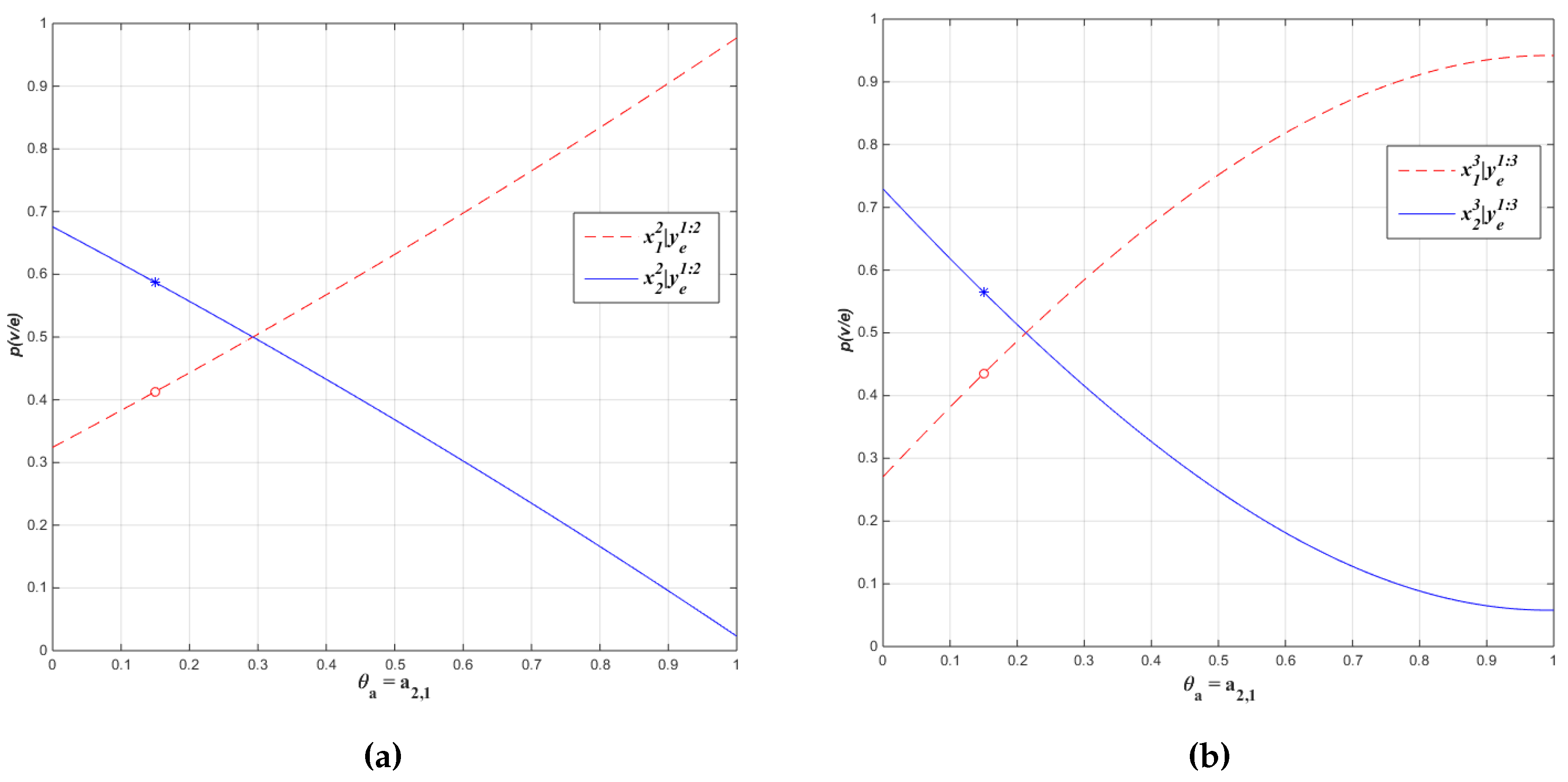
these sensitivity functions are displayed in Figure 2.
The derivative of these sensitivity functions can be used to analyze the sensitive of the filtering tasks for the change in parameter .
and
3.5. Run-time Analysis
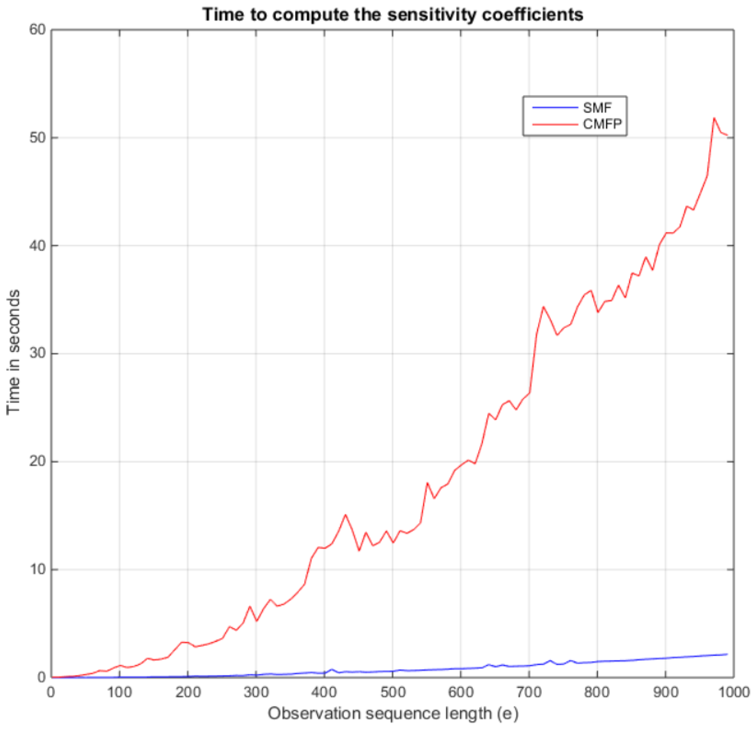
The time for computing the coefficients of the filtering probabilities for transition parameter variation is recorded for the Coefficient-Matrix-Fill procedure and our method (SMF) using the HMM shown in Example (1). It is shown in Figure 3, where the Coefficient-Matrix-Fill procedure is labled as CMFP. In [26], the algorithm for the Coefficient-Matrix-Fill procedure is presented. It is shown for an HMM model with hidden states and observable symbols. The proposed SMF algorithm has shown a significant improvement in computational time compared to the Coefficient-Matrix-Fill procedure as the length of the observation sequence increases. For example, for an observation sequence length of 1000, the proposed technique takes a mean time of 0.048 s. In comparison, it takes the Coefficient-Matrix-Fill procedure 2.183 seconds. This is an improvement of 98%. The algorithms are implemented in MATLAB on a 64-bit Windows 7 Professional Workstation (Dell Precision T7600 with Intel(R) Xeon CPU E5-2680 0 @ 2.70 GHz dual core processors and 64GB RAM).
The computational complexity of our method is linear time, , where l is the length of the observation sequence, whereas the Coefficient-Matrix-Fill procedure is quadratic time, . In our method, the sensitivity function coefficients are computed in one for loop that runs for the length of the observation sequence, as shown in Algorithms 1–6, whereas in the Coefficient-Matrix-Fill procedure two nested for loops are used. It computes the sensitivity coefficients in the forward matrices element-by-element in the inner loop, which runs in increasing time up to the maximum of the length of the observation sequence, and the outer loop runs for the length of the observation sequence.
4. Sensitivity Analysis of Smoothing Probability
In this section, the sensitivity analysis of smoothing probability for variation of the transition, initial and observation parameters are presented using simplified matrix formulation. The sensitivity function where and is one of the model parameters, can be computed using the recursive probability expression shown in Equation (2) and (3).
The first term in this product can be computed using the backward procedure as shown in Equation (3); the second term is the filtering probability that is computed using the forward procedure. Consequently, the sensitivity function for the smoothing probability is the product of the polynomial sensitivity functions computed using the forward and backward procedures. The sensitivity function for the filtering probability is discussed in Section 3. From Equation (3), the backward recursive probability expression, it follows that
where
and
To compute the coefficients of the sensitivity function , a series of Backward matrices based on the simplified matrix formulation as presented in Section 3 are used. In the next subsections, the sensitivity functions for the smoothing probability for transition, initial and observation parameter variations are discussed.
4.1. Transition Parameter Variation
In the simplified matrix formulation, the sensitivity function for transition parameter can be represented as follows:
For , , the recursive probability expression reduces to the following:
The proposed technique for the sensitivity analysis of the backward probability sensitivity function for the transition parameter is formulated in Algorithm 4.
| Algorithm 4 This computes the coefficients of the backward probability sensitivity function in backward matrices for using SMF. |
| Input: |
| Output: |
|
4.1.1. Algorithm Implementation
In this algorithm, e is the sequence of observation and . It solves the recursive backward probability sensitivity function Equation (10) using the backward matrices for . Once the transition matrix is decomposed into the transition matrices independent of and dependent on , the coefficients of the sensitivity function are computed by filling the backward matrices as follows. First, is initialized as a vector of ones for n hidden states.
The remaining matrices of size are computed by filling them as follows: Once the observation matrix is represented as a diagonal matrix, two temporary matrices and are used for computing the coefficients as previously explained. is computed as the matrix multiplication of that is independent of , and and a zero vector of size n is appended at its end. represents the recursion in the backward probability. The same way is computed as the matrix multiplication of that is dependent on , and and a zero vector of size n is appended to the front. Then is set as the sum of and ,
4.2. Initial Parameter Variation
In this subsection, the sensitivity of the backward probability to initial parameter variation is derived based on SMF. The sensitivity function for initial parameter variation , as shown in the recursive backward probability sensitivity function in Equation (10), can be represented in SMF as
For , and the recursive probability expression reduces to
The procedure to compute the coefficients of the function in backward matrices for using SMF is summarized in Algorithm 5.
| Algorithm 5 This computes the coefficients of the backward probability sensitivity function with in backward matrices for using SMF. |
| Input: |
| Output: |
|
4.2.1. Algorithm Implementation
As discussed above, the sensitivity function for the backward probability with is a polynomial of degree zero. The contents of the backward matrices are filled as follows. is initialized as a vector of ones for n hidden states.
The remaining matrices of size are computed by filling them as follows. Once the observation matrix is represented as a diagonal matrix, is set as the matrix multiplication of A, and . represents the recursion in the backward probability.
4.3. Observation Parameter Variation
The sensitivity function for the backward probability for the observation parameter variation can be represented as follows:
For , , the recursive probability expression reduces to the following
The sensitivity analysis of the backward probability sensitivity function for observation parameter variation is summarized in Algorithm 6.
| Algorithm 6 This computes the coefficients of the backward probability sensitivity function with in backward matrices for using SMF. |
| Input: |
| Output: |
|
4.3.1. Algorithm Implementation
In this algorithm, e is the sequence of observation and and it solves the recursive backward probability sensitivity function Equation (10) in the backward matrices for using SMF. Once the observation matrix is decomposed into the independent and dependent observation matrices on , the coefficients of the sensitivity function are computed by filling the backward matrices as follows: is initialized as a vector of ones for n hidden states.
The remaining matrices of size are computed by filling them as follows: Once the independent and dependent observation matrices on is represented as a diagonal matrix, two temporary matrices and are used for computing the coefficients of the sensitivity function as previously explained. is computed as the matrix multiplication of A, and . A zero vector of size n is appended at its end. represents the recursion in the backward probability. In the same way is computed as the matrix multiplication of A, and and a zero vector of size n is appended to the front. Then is set as the sum of and ,
5. Conclusions and Future Research
This research has shown that it is more efficient to compute the coefficients for the HMM sensitivity function directly from the HMM representation. The proposed method exploits the simplified matrix formulation for HMMs. A simple algorithm is presented which computes the coefficients for the sensitivity function of filtering and smoothing probabilities for transition, initial and observation parameter variation for all hidden states, as well as all time steps. This method differs from the other approaches in that it neither depends on a specific computational architecture nor requires a Bayesian network representation of the HMM.
The future extension of this work will include sensitivity analysis of predicted future observations , and the most probable explanation for the corresponding parameter variations. Future research on the sensitivity analysis of HMM, where different types of model parameters are varied simultaneously, as well as the case of continuous observations will be considered.
Acknowledgments
This work is partially supported by the US Department of Transportation (USDOT) under University Transportation Center (UTC) Program (DTRT13-G-UTC47), the Office of the Secretary of Defense (OSD) and the Air Force Research Laboratory under agreement number FA8750-15-2-0116. The U.S. Government is authorized to reproduce and distribute reprints for Governmental purposes, notwithstanding any copyright notation thereon. The views and conclusions contained herein are those of the authors and should not be interpreted as necessarily representing the official policies or endorsements, either expressed or implied, of USDOT, OSD, Air Force Research Laboratory, or the U.S. Government. The first, and the second authors would like to acknowledge the support from the USDOT, and the second author would also like to acknowledge the support from the OSD and the Air Force.
Author Contributions
Seifemichael B. Amsalu and Abdollah Homaifar contributed equally to this work. Albert C. Esterline helped in writing the manuscript; All authors have read and approved the final manuscript.
Conflicts of Interest
The authors declare no conflicts of interest exist in this work.
References
- Patel, I.; Rao, Y.S. Speech recognition using hidden Markov model with MFCC-subband technique. Recent Trends Inf. Telecommun. Comput. 2010, 5, 168–172. [Google Scholar]
- Birney, E. Hidden Markov models in biological sequence analysis. IBM J. Res. Dev. 2001, 45, 449–454. [Google Scholar] [CrossRef]
- Mamon, R.S.; Elliott, R.J. Hidden Markov models in finance. In International Series in Operations Research & Management Science, 2nd ed.; Springer: New York, NY, USA, 2014; Available online: https://link.springer.com/book/10.1007/978-1-4899-7442-6 (accessed on 11 August 2017).
- Bunke, H.; Caelli, T. Hidden Markov Models: Applications in Computer Vision; World Scientific Publishing: Danvers, MA, USA, 2001; pp. 1–223. [Google Scholar]
- Amsalu, S.B.; Homaifar, A.; Afghah, F.; Ramyar, S.; Kurt, A. Driver behavior modeling near intersections using support vector machines based on statistical feature extraction. Intell. Veh. Symp. 2015, 8, 1270–1275. [Google Scholar]
- Amsalu, S.B.; Homaifar, A. Driver behavior modeling near intersections using hidden Markov model based on genetic algorithm. Intell. Transp. Eng. 2016, 10, 193–200. [Google Scholar]
- Dymarski, P. Hidden Markov Models, Theory and Applications; InTech Open Access Publishers: Vienna, Austria, 2011; pp. 1–9. Available online: https://cdn.intechopen.com/pdfs-wm/15359.pdf (accessed on 11 August 2017).
- Murphy, K.P. Bayesian Networks: Representation, Inference and Learning. Ph.D. Thesis, University of California, Berkeley, CA, USA, 2002. [Google Scholar]
- Smyth, P.; Heckerman, D.; Jordan, M.I. Probabilistic independence networks for hidden Markov probability models. Neural Comput. 1997, 9, 227–269. [Google Scholar] [CrossRef] [PubMed]
- Coquelin, P.A.; Deguest, R.; Munos, R. Sensitivity analysis in HMMs with application to likelihood maximization. Adv. Neural Inf. Process. Syst. 2009, 22, 387–395. [Google Scholar]
- Mitrophanov, A.Y.; Lomsadze, A.; Borodovsky, M. Sensitivity of hidden Markov models. J. Appl. Probab. 2005, 42, 632–642. [Google Scholar] [CrossRef]
- Chan, H.; Darwiche, A. A distance measure for bounding probabilistic belief change. Int. J. Approx. Reason. 2005, 38, 149–174. [Google Scholar] [CrossRef]
- Renooij, S.; Van der Gaag, L.C. Evidence-invariant sensitivity bounds. Uncertain. Artif. Intell. 2004, 7, 479–486. [Google Scholar]
- Renooij, S.; Van der Gaag, L.C. Exploiting evidence-dependent sensitivity bounds. Uncertain. Artif. Intell. 2012. Available online: https://arxiv.org/abs/1207.1357 (accessed on 11 August 2017).
- Renooij, S.; Van der Gaag, L.C. Evidence and scenario sensitivities in naive Bayesian classifiers. Int. J. Approx. Reason. 2008, 49, 398–416. [Google Scholar] [CrossRef]
- Chan, H.; Darwiche, A. When do numbers really matter? J. Artif. Intell. Res. 2002, 17, 265–287. [Google Scholar]
- Van der Gaag, L.C.; Renooij, S.; Coupé, V.M.H. Sensitivity analysis of probabilistic networks. In Advances in Probabilistic Graphical Models; Springer: Berlin, Germany, 2007; pp. 103–124. [Google Scholar]
- Laskey, K.B. Sensitivity analysis for probability assessments in Bayesian networks. IEEE Trans. Syst. Man Cybern. 1995, 25, 901–909. [Google Scholar] [CrossRef]
- Jensen, F.V.; Nielsen, T.D. Bayesian Networks and Decision Graphs, 2nd ed.; Springer: Berlin, Germany, 2007; pp. 1–441. [Google Scholar]
- Darwiche, A. A differential approach to inference in Bayesian networks. J. Assoc. Comput. Mach. 2003, 50, 280–305. [Google Scholar] [CrossRef]
- Coupé, V.M.H.; Jensen, F.V.; Kjærulff, U.; Van der Gaag, L.C. A computational architecture for N-way sensitivity analysis of Bayesian networks. Dep. Comput. Sci. 2000. Available online: http://citeseerx.ist.psu.edu/viewdoc/summary?doi=10.1.1.34.1434 (accessed on 11 August 2017).
- Kjærulff, U.; Van der Gaag, L.C. Making sensitivity analysis computationally efficient. In Uncertainty in Artificial Intelligence; Morgan Kaufmann: San Francisco, CA, USA, 2000; pp. 317–325. [Google Scholar]
- Chan, H.; Darwiche, A. Sensitivity analysis in Bayesian networks: Fromsingle to multiple parameters. In Uncertainty in Artificial Intelligence; AUAI Press: Arlington, VA, USA, 2004; pp. 67–75. [Google Scholar]
- de Cooman, G.; Hermans, F.; Quaeghebeur, E. Sensitivity analysis for finite Markov chains in discrete time. Uncertain. Artif. Intell. 2008, 8, 129–136. [Google Scholar]
- Renooij, S. Efficient sensitivity analysis in hidden Markov models. In Proceedings of the Fifth European Workshop on Probabilistic Graphical Models; HIIT Publications: Helsinki, Finland, 2010; pp. 241–248. Available online: http://www.cs.uu.nl/research/techreps/repo/CS-2011/2011-025.pdf (accessed on 19 August 2017).
- Renooij, S. Efficient sensitivity analysis in hidden Markov models. Int. J. Approx. Reason. 2012, 53, 1397–1414. [Google Scholar] [CrossRef]
- Maua, D.; de Campos, C.; Antonucci, A. Algorithms for hidden Markov models with imprecisely specified parameters. Br. Conf. Intell. Syst. 2014, 186–191. [Google Scholar] [CrossRef]
- Baum, L.E.; Petrie, T. Statistical inference for probabilistic functions of finite state Markov chains. Ann. Math. Stat. 1966, 37, 1554–1563. [Google Scholar] [CrossRef]
- Rabiner, L.R. A tutorial on hidden Markov models and selected applications in speech recognition. Proc. IEEE 1989, 77, 257–286. [Google Scholar] [CrossRef]
- Bilmes, J. A gentle tutorial on the EM algorithm and its application to parameter estimation for Gaussian mixture and hidden Markov models. Int. Comput. Sci. Inst. 1998, 4, 126. [Google Scholar]
- Russell, S.; Norvig, P. Artificial Intelligence: A Modern Approach, 3rd ed.; Prentice Hall: New Jersey, NJ, USA, 2010; pp. 1–1154. [Google Scholar]
- Charitos, T.; Van der Gaag, L.C. Sensitivity properties of Markovian models. In Proceedings of Advances in Intelligent Systems—Theory and Applications Conference (AISTA); IEEE Computer Society: Luxembourg, 2004; Available online: https://pdfs.semanticscholar.org/5d53/1a739b047fa6a126dfa32ba5ccccd3f5934c.pdf (accessed on 11 August 2017).
- Van der Gaag, L.C.; Renooij, S. Analysing sensitivity data from probabilistic networks. Uncertain. Artif. Intell. 2001, 530–537. Available online: http://dl.acm.org/citation.cfm?id=2074087 (accessed on 11 August 2017).
Figure 1.
(a) An example of an HMM representation. (b) Its dynamic Bayesian network representation, unrolled for T time slices.
Figure 1.
(a) An example of an HMM representation. (b) Its dynamic Bayesian network representation, unrolled for T time slices.
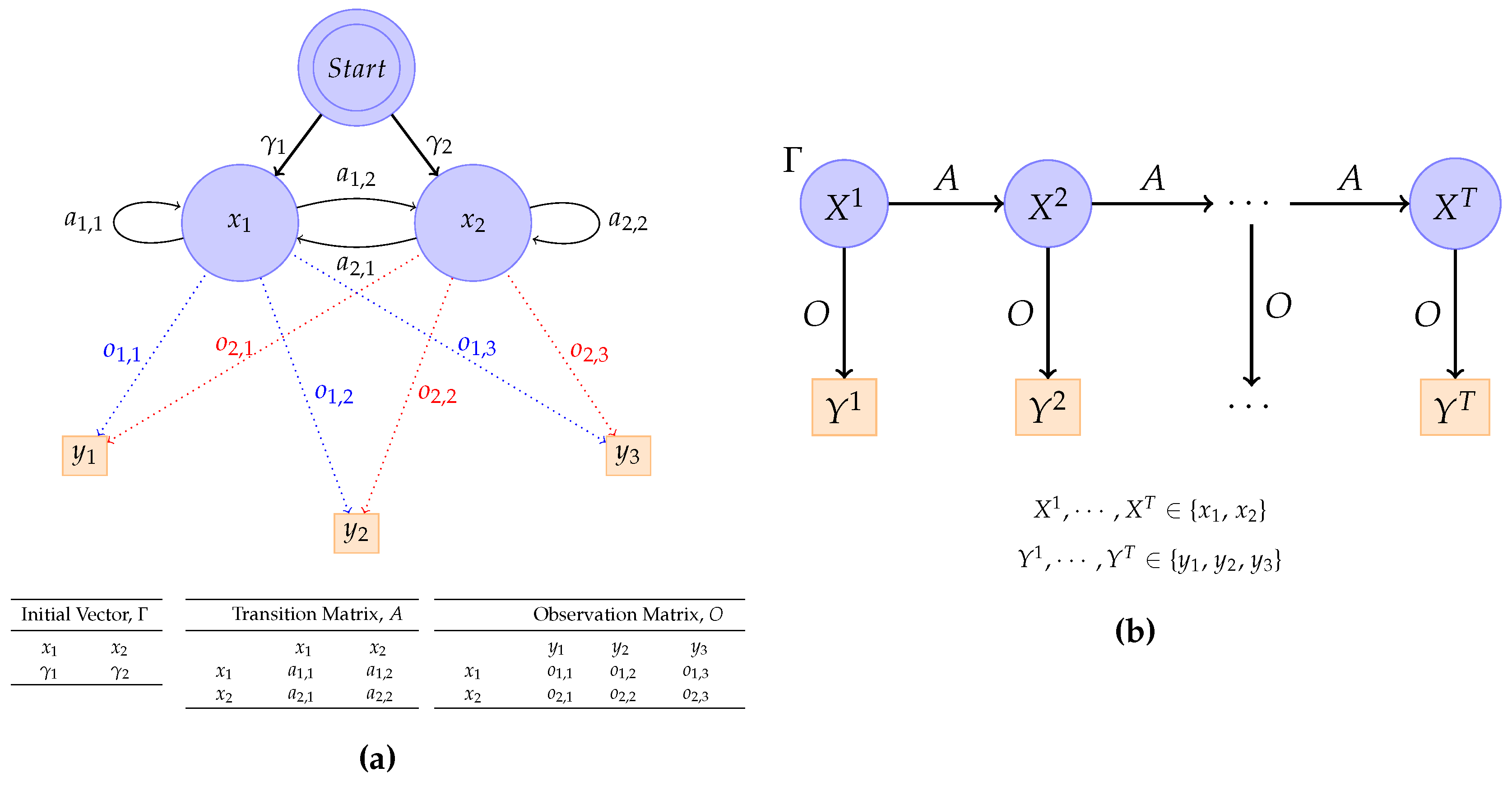
Figure 2.
Sensitivity functions: (a) for both states of . (b) for both states of .

Figure 3.
Time in seconds to compute the sensitivity coefficients for an observation sequence length from 1 to 1000 with a step size of 10.
Figure 3.
Time in seconds to compute the sensitivity coefficients for an observation sequence length from 1 to 1000 with a step size of 10.

© 2017 by the authors. Licensee MDPI, Basel, Switzerland. This article is an open access article distributed under the terms and conditions of the Creative Commons Attribution (CC BY) license (http://creativecommons.org/licenses/by/4.0/).
Share and Cite
MDPI and ACS Style
Amsalu, S.; Homaifar, .; Esterline, A.C. A Simplified Matrix Formulation for Sensitivity Analysis of Hidden Markov Models. Algorithms 2017, 10, 97. https://doi.org/10.3390/a10030097
AMA Style
Amsalu S, Homaifar , Esterline AC. A Simplified Matrix Formulation for Sensitivity Analysis of Hidden Markov Models. Algorithms. 2017; 10(3):97. https://doi.org/10.3390/a10030097
Chicago/Turabian StyleAmsalu, Seifemichael B., Abdollah Homaifar, and Albert C. Esterline. 2017. "A Simplified Matrix Formulation for Sensitivity Analysis of Hidden Markov Models" Algorithms 10, no. 3: 97. https://doi.org/10.3390/a10030097
Note that from the first issue of 2016, this journal uses article numbers instead of page numbers. See further details here.