Development of Filtered Bispectrum for EEG Signal Feature Extraction in Automatic Emotion Recognition Using Artificial Neural Networks

Abstract

The development of automatic emotion detection systems has recently gained significant attention due to the growing possibility of their implementation in several applications, including affective computing and various fields within biomedical engineering. Use of the electroencephalograph (EEG) signal is preferred over facial expression, as people cannot control the EEG signal generated by their brain; the EEG ensures a stronger reliability in the psychological signal. However, because of its uniqueness between individuals and its vulnerability to noise, use of EEG signals can be rather complicated. In this paper, we propose a methodology to conduct EEG-based emotion recognition by using a filtered bispectrum as the feature extraction subsystem and an artificial neural network (ANN) as the classifier. The bispectrum is theoretically superior to the power spectrum because it can identify phase coupling between the nonlinear process components of the EEG signal. In the feature extraction process, to extract the information contained in the bispectrum matrices, a 3D pyramid filter is used for sampling and quantifying the bispectrum value. Experiment results show that the mean percentage of the bispectrum value from 5 × 5 non-overlapped 3D pyramid filters produces the highest recognition rate. We found that reducing the number of EEG channels down to only eight in the frontal area of the brain does not significantly affect the recognition rate, and the number of data samples used in the training process is then increased to improve the recognition rate of the system. We have also utilized a probabilistic neural network (PNN) as another classifier and compared its recognition rate with that of the back-propagation neural network (BPNN), and the results show that the PNN produces a comparable recognition rate and lower computational costs. Our research shows that the extracted bispectrum values of an EEG signal using 3D filtering as a feature extraction method is suitable for use in an EEG-based emotion recognition system.

1. Introduction

It is widely believed that psychological factors can affect a patient’s recovery process; positive emotions, for example, affect the progression of recovery, and a patient’s emotional response to his or her illness could also affect the type and amount of medication prescribed by doctors [1]. Psychological treatment is one of the most important factors in a patient’s recovery and, when administered properly, might even accelerate the healing process. Although psychologists are still debating whether positive emotions could cure patients suffering from life-threatening illnesses, experts believe that experiencing positive emotions (e.g., feeling happy and stress free) would improve patients’ social life, which in turn make patients more productive in their daily activities.

The difficulty in utilizing the psychological approach in the patient recovery process stems from the patient’s ability to hide emotions or the inability to express an emotional condition despite his or her desires, such as cases where patients experience facial nerve paralysis or adhere to certain cultural dynamics. When these situations occur, even social approaches through various communication techniques or observations of body language still pose a challenge, as the nurse or the patient’s family members might not be able to accompany the patient at all times. A solution can therefore be found in an automatic emotion recognition tool or system.

There are several ways to determine human emotions automatically. One popular way is by using a camera and image processing technique to recognize facial expressions; however, this method is ineffective when patients suffer from facial paralysis or when they hide their genuine emotions. Therefore, another approach should be considered, such as automatic emotion recognition that incorporates the use of physiological signals, such as the electrocardiograph (ECG) for monitoring the patient’s heart rate, the multi-resonance imaging (f-MRI) for monitoring blood-oxygen-level dependence (BOLD), the eye-gaze trackers (EGT) for monitoring the width of the pupil movements or the EEG for monitoring brain signals. The EEG-based emotion recognition system is preferred due to the advantage of its temporal resolution [2] and the ability of the patient to move around while the EEG-based emotion recognition system is processing the signals.

The goal of this research is to develop an automatic system for recognizing human emotions through EEG signals. The power spectrum analysis has previously been implemented in the developed automatic emotion recognition system [3], and in this work, the bispectrum analysis, which theoretically is better than the power spectrum analysis, was used as the feature extraction subsystem, while ANNs served as the classifiers. For the purpose of benchmarking the experiment setup and comparing the recognition capability of the developed system, we have used the EEG signals from healthy subjects as provided by the Database for Emotion Analysis Using Physiological Signals (DEAP) [4].

The rest of the paper is organized as follows: Section 2 presents the literature review on methodologies previously proposed by other researchers; Section 3 discusses the methodology used in this research, the materials of the study, the bispectrum processing technique, including the proposed 3D filtering method for extracting the bispectrum value, and the classifiers used (i.e., the BPNN and the PNN); Section 4 describes in detail the experimental method and discusses the results; finally, Section 5 concludes the paper.

2. Literature Review

Researchers have proposed many different methods for recognizing emotions through EEG signals [2,5]. The fundamental challenge of using EEG signals to detect human emotion lies in understanding how a particular emotional state is represented in the brain and applying the correct computational model to accurately identify that emotion, both automatically and in real time. Human emotion is naturally felt after a few seconds, not in a split second; therefore, it is more appropriate if the EEG signals used for the analysis have a set time frame to avoid analyzing the signals’ amplitude as in the event-related potentials (ERP) technique. However, the ERP technique has been used in other emotion recognition research [6,7,8,9] because the emotional stimuli were instantaneous pictures. On the other hand, to analyze EEG signals within a certain time duration for successful and productive use in an emotion recognition system, a signal processing technique is needed: one widely-adopted method is to calculate the power spectrum of the brain signals [4,10,11,12,13], and the results were an approximately 60–70% recognition rate, showing much room for improvement.

Bispectrum analysis has been used as a signal processing technique for analyzing the EEG signal [14] and also used in medical research, such as in cases related to anesthesia [15,16], meditation [17], vigilance tests [18] and recently in emotion recognition [19,20], but the recognition rate result for the latter was somewhat lower than desired. Hosseini [19] used seven features from bispectrum analysis taken from each of five EEG channels to recognize whether the subject was stressed; Hosseini used a support vector machine (SVM) as the classifier and a genetic algorithm as the feature selection algorithm. Kumar [20] used the bispectrum as a feature extraction method to identify four types of emotional states, namely the low and high arousal and the low and high valence from the data provided in the DEAP database [4], using only two channels (Fp1 and Fp2) as the input signals and SVM as the classifier. There were five types of features calculated after the bispectrum analysis: normalized bispectral entropy (NBE), normalized bispectral squared entropy (NBSE), mean-magnitude of bispectrum (MMOB), first order spectral moment (FOSM) and second order spectral moment (SOSM). However, the use of a higher complexity feature calculation leads to an increased computation cost and may result in decreased accuracy. In this work, we propose a simpler method for feature extraction after the bispectrum values are calculated: to calculate the mean of bispectrum values after they are divided, by a filtering method, into several spatial regions, and using the percentage of the mean as the feature.

Regarding the relationship between EEG and emotion, the prefrontal cortex area of the brain exhibits a strong correlation with human emotion. Nevertheless, through the feature selection process, some researchers have found that other EEG channels were better suited for emotion recognition [20,21]. In the frequency domain, particular emotions are believed to affect specific frequency bands, such as alpha [22,23], gamma [24,25] and theta [26], and some researchers have incorporated all frequencies, delta, alpha, beta, theta and gamma [19,27], into their EEG research. In this work, we used all frequencies of brain signals and omitted none.

For the EEG signal classification using DEAP as the dataset, both linear and non-linear methods have been used widely; such as support vector machine (SVM) [28,29,30,31,32], linear discriminant analysis (LDA) [33], quadratic discriminant analysis (QDA) [30], k-nearest neighbor (KNN) [34] for the linear classifier; and back-propagation neural networks (BPNN) [3], probability neural networks (PNN) [35], Bayesian neural networks (BNN) [36], deep learning networks (DLN) [37] and Elman neural networks (ENN) [19] for the non-linear classifier. In this work, we use the BPNN as the benchmark classifier. Although BPNN has a major drawback in terms of time, it is guaranteed to execute the best performance because the algorithm uses a gradient descent of error. We also compared our classification results using BPNN to the results with that of the PNN.

DEAP has been used by many researchers because a complete description of the data acquisition is available, the data samples are large enough, i.e., 1280 samples, and the pre-processed data in the form of MATLAB and Python matrices are also provided; these allow researchers to be focused on the development of feature extraction and the classification methods. However, the results achieved by different researchers are difficult to compare because they use various cross-validation methods, and the recognition rate result varied between 40% and 90%.

3. Bispectrum Analysis of EEG Signals for an Emotion Recognition System

There is a significant amount of research focusing on human emotion recognition. However, only a few publicly open databases of emotion are available for download, and in this research, we chose the DEAP database [4] for two reasons. First, the DEAP database uses carefully-chosen emotional stimuli based on statistical methods from the respondents. To ensure objectivity, the respondents who assessed the emotional stimuli were different from the respondents who recorded the EEG signals. Second, this database provides numerous observations. Using a publicly open database enables us to reproduce and compare our research results with other findings.

To recognize human emotion automatically, the proposed method employs higher order statistics to the EEG signal to produce 3D bispectrum matrices. Then, the bispectrum matrices are filtered using a 3D pyramid filter to reduce the size of the matrices and to form a feature vector. The resulting feature vectors are used as the input for the BPNN classifier.

3.1. EEG Database and Its Acquisition

Currently, the existing EEG databases available for research purposes mostly contain the EEG signals of motor imagination [38,39], sleep stages [40] and epilepsy [41], and only a few EEG databases related to the emotional states are available, such as Mahnob-HCI [42], the SJTU Emotion EEG Dataset (SEED) database [43] and the DEAP database [4]. This work utilized the DEAP database [4] that provided the most EEG data from participants; emotional stimuli came from video music clips, and the emotional states of the participants were defined in 2D emotion models (i.e., the arousal and the valence levels [4]), producing four quadrants of emotion: the high arousal, high valence (HAHV); the low arousal, high valence (LAHV); the low arousal, low valence (LALV); and the high arousal, low valence (HALV) emotion classes.

In this database, the emotional stimuli for each quadrant of the 2D emotion model were portioned equally with 10 music videos, and the excited EEG signals from the brain activity were recorded using 32 channels of an EEG Biosemi ActiveTwo with a sampling rate of 512 Hz. The DEAP database also provided a list of the videos and their YouTube URLs, the basic statistics of participants’ ratings, the physiological signals, the facial expression videos and the preprocessed data. EEG signals were recorded from 32 people (balance between women and men) between the ages of 19 and 37 years. During the recording process, each participant was asked to rate, on a scale of 1–9, his or her emotional response when watching the video in terms of arousal, valence, likes/dislikes, the dominance and the familiarity through the Self-Assessment Manikin (SAM) questionnaire [4].

As EEG signals are vulnerable to noises, several noise filtering methods, such as to remove power line noise, eye and muscle artefact removal [44,45], are usually applied. In DEAP, several pre-processing steps that consist of a band-pass filtering at 50 Hz and 60 Hz, a high-pass filtering at 2 Hz, a down-sampling process to 128 Hz and the removal of artefacts corresponding to electrooculography (EOG) have been conducted [4]. The DEAP database then provides 32 matrices of 40 × 40 × 8064, representing video/trial × physiology channels × duration of the signals, respectively; however, for our research purposes, these original 32 matrices were divided into a 1280 person-video data matrix (32 people × 40 videos). In this work, we only considered the EEG signals; thus, only 32 out of 40 physiology signals are used, and we eliminated the first three-second baseline from the 63-second duration of the signals, so the resulting size of each matrix was 32 × 7680 (EEG channels × duration of the signals). The 1280 matrices were further divided into 320 matrices (32 people × 10 videos) for each class of emotion.

3.2. EEG Channel Selection Related to Human Emotion

The brain is the operations center of the human nervous system and can be divided into three major parts: the brainstem, the cerebellum (hindbrain) and the cerebrum (front brain). The largest part of the brain is the cerebrum, and the outer part of the cerebrum is the cerebral cortex, which generates most of the voltage measured on the surface of the head. The cerebral cortex is divided into four lobes, which are the temporal, the frontal, the parietal and the occipital lobes. Each lobe is associated with various functions, and the frontal lobe is where we can observe brain signals associated with emotions.

An EEG captures the electrical activity of the brain by measuring the voltage fluctuations due to the flow of the electric current between neurons in the brain. The EEG electrodes are named according to their corresponding area of the cerebral cortex: the frontal (F), the central (C), the parietal (P), the occipital (O) and the temporal (T). Some electrodes are placed in pairs on the left side and right side of the head, with odd numbers given to the left electrode positions and even numbers given to the right electrode positions. The electrodes in the middle positions are given zero (z) subscripts.

In this study, we document the effect of channel selection on the recognition rate of the emotion classification system; then, aside from the initial 32 channels, we also assess the effect of channel selection on the brain emotion theory, which involves all eight channels on the frontal, frontal parietal and anterior-frontal regions. In addition to studying the 32 channels and the reduced eight channels, we also compared our results with the 14 channels corresponding to the channels available in the BCI Emotiv device.

3.3. The Developed Methodology for Emotion Classification System

Generally, the automatic emotion recognition process can be carried out using classification algorithms through a mathematical-based machine learning method or through a biological-based ANN method. Using both learning mechanisms of the classification algorithms, the researchers’ main focus is finding the best techniques for the feature extraction subsystem in order to minimize classification error and improve the recognition rate.

The developed methodology for our automatic emotion recognition system is illustrated in Figure 1. At the first stage, human emotions are elicited through a set of emotion stimuli, usually by pictures, sounds or videos. Then, the EEG input signals are captured by an EEG device with several electrodes using the appropriate sampling frequency. In this research, the EEG input signals were provided by the DEAP database, and these signals were stimulated by a set of music videos (clips). The EEG input signals from this database were already preprocessed [3] through certain steps, such as reducing interference noise during the EEG recording, including power line frequency noise filtering and the blink artefact removal.

To retrieve any meaningful information hidden in the EEG signal, the original time domain signals are processed using some signal processing techniques, and the features are then calculated and extracted. Because the higher spectrum analysis is theoretically better than the power spectrum model, we processed our signals using bispectrum analysis, and to reduce the bispectrum matrix size, we also applied a 3D filtering method. The features are extracted by calculating several relevant pieces of information from the filtered bispectrum matrix, such as the entropy, the moment and the mean. The best features are then investigated further to determine the highest recognition rate.

As the feature vectors produced by bispectrum analysis are usually larger than that of the power spectrum analysis, the higher computation cost of using bispectrum analysis could not be avoided. To reduce the size of the feature vectors, and in turn reduce the computation cost, a principal component analysis (PCA) technique that searches the best principal components (i.e., the coefficient matrix according to the number of the Eigen values desired) is utilized. We also sought to determine whether reduction in the number of channels used could contribute to reducing the computation cost without decreasing the recognition rate.

In the classification stage, the BPNN classifier was chosen as the benchmark classifier among other ANN classifiers due to its capacity to guarantee the convergence of the minimum error using a gradient descent training method. We then compared the performance of the BPNN with another ANN classifier, namely the PNN, that uses Bayesian probability in the classification process.

3.4. Feature Extraction Based on Bispectrum Analysis and 3D Pyramid Filter

3.4.1. Bispectrum

The power spectrum analysis, which has been widely used in biomedical signal processing, performs power distribution calculation using a function of frequency and pays no attention to the signal phase information. In the power spectral analysis, the signal is assumed to arise from a linear process, thus ignoring any possible interaction between components (phase coupling). However, the brain signal is part of the central nervous system with many nonlinear sources, so it is highly likely to have a phase coupling between signals [14]. The bispectrum analysis is superior to the power spectrum analysis because in its mathematical formula, there is a correlation calculation between the frequency components [46]; thus, the phase coupling components of the EEG signals could be revealed. Some characteristics of bispectrum analysis are the ability to extract deviations due to Gaussianity, to suppress the additive colored Gaussian noise of an unknown power spectrum and to detect nonlinearity properties [47]. Because of its superiority, bispectrum analysis is used in this research as the signal processing technique in the feature extraction step. We expect that by using bispectrum analysis, the recognition rate of the EEG-based automatic emotion recognition system will improve.

For example, suppose there is a signal S₃ that is a combination of two other signals, S₁ and S₂, where the frequencies are f₁ = 20 Hz, f₁ = 10 Hz and f₃ = f₁ + f₂ = 30 Hz, and the phases are φ₁ = π/6, φ₂ = 5π/8 and φ₃ = φ₁ + φ₂, respectively. The signals S₁, S₂ and S₃ are then defined as follows: S₁ = 3 cos(2πf₁t + φ₁), S₂ = 5 cos(2πf₂t + φ₂) and S₃ = 8 cos(2πf₃t + φ₃). The resulting signal X(t) = S₁ + S₂ + S₃ is then received by a sensor. 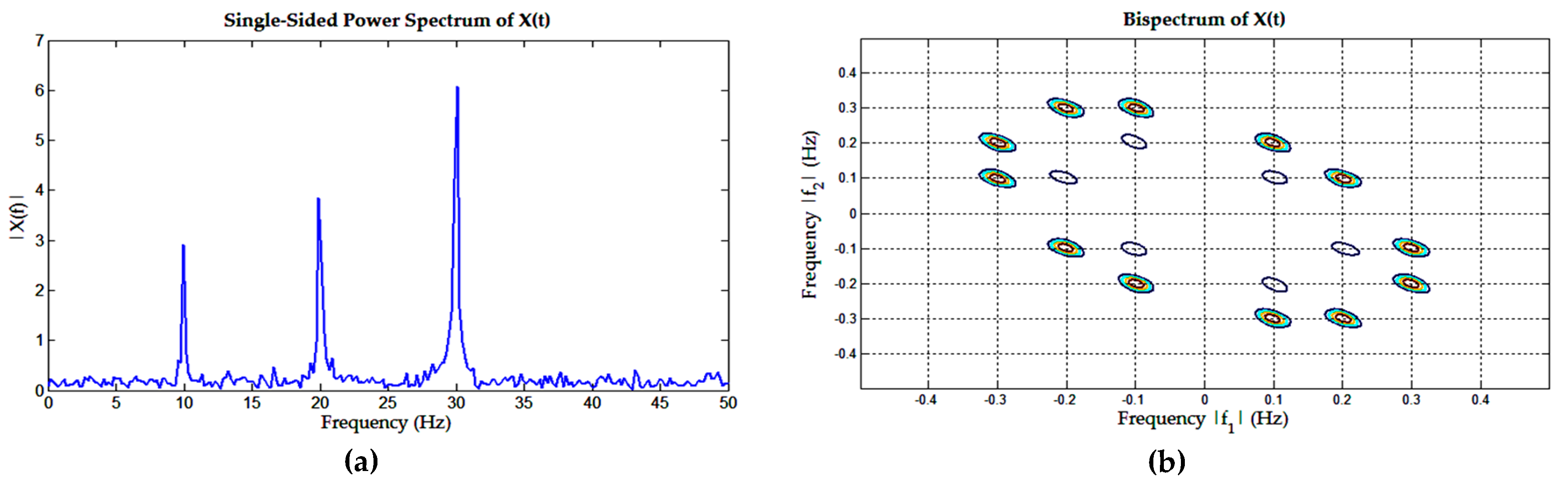With the sampling frequency of 100 Hz, signal X(t) is processed to reveal its power spectrum and its bispectrum values, and the result can be seen in Figure 2. The power spectrum (Figure 2a) produced using FFT showed that the dominant frequencies are 10, 20 and 30 Hz; however, it does not reveal the fact that the frequency 30 Hz is a resulting combination of frequencies 10 and 20 Hz. On the other hand, in bispectrum (Figure 2b), the pair of normalized frequencies 0.1 and 0.2 Hz (equal to the original frequencies 10 and 20 Hz), on coordinate (0.1,0.2) and (0.2,0.1), show a high spectrum, which means that they are strongly correlated because they produce the 30-Hz signal. Supposing that the signal S₃ is noise, by using a bispectrum analysis, the noise signal will not be taken into consideration. Thus, we can conclude that through bispectrum analysis, the main frequency components are revealed while the other frequencies are eliminated. Because bispectrum analysis provides more information than the power spectrum analysis, it is expected that the use of bispectrum analysis in the EEG signals’ feature extraction process will increase the recognition rate.

The autocorrelation of a signal is the correlation between the signal and itself at a different time; for example, at time t and at time t + m. The autocorrelation function of x(n) can be expressed as the expectation of stationary process, defined as:

$$R_{xx}\left(m\right):=E\left\{x^{*}\left(n\right)x\left(n+m\right)\right\}.$$

(1)

The higher order moments are a natural generalization of autocorrelation, and the cumulants are a nonlinear combination of moments. The first order cumulant (C_1x) from stationary process is the mean, C_1x = E {x(t)}, with E{.} an expectation notation. The higher order cumulants have the property invariant to the shift of the mean; therefore, it is practical to describe the cumulants under zero mean assumption, meaning that if the mean of a process is not zero, then as the first step, the mean should be subtracted from each value. The second order polyspectrum, which is the power spectrum, is defined as the Fourier transform of the second order cumulant, while the third order polyspectrum, which is the bispectrum, is defined as the Fourier transform of the third order cumulant.

For the third order cumulant, the autocorrelation of a signal will be calculated until the distance t + τ₁ and t + τ₂, where τ₁ and τ₂ are the lag. The third order cumulant from a zero mean stationary process is defined as [48]:

$$C_{3x}\left({\tau }_1,{\tau }_2\right)=E\left\{x^{*}\left(n\right)x\left(n+{\tau }_1\right)x\left(n+{\tau }_2\right)\right\}.$$

(2)

Thus, the bispectrum, $B\left(f_1,f_2\right)$, defined as the Fourier transform of the third order cumulant, becomes:

$$B\left(f_1,f_2\right)={{\displaystyle \sum }}_{k=-\infty }^{\infty }{{\displaystyle \sum }}_{l=-\infty }^{\infty }{C}_{2x}\left(k\right)e^{-j2\pi f_{1}k}{e}^{-j2\pi f_{2}l}.$$

(3)

The bispectrum has a specific symmetrical property that is derived from the symmetrical property of the third order cumulant [46], which results in similarity of the six regions of the bispectrum, shown as follows:

$$\begin{array}{cc}\hfill C_{3x}\left({\tau }_1,{\tau }_2\right)& =C_{3x}\left({\tau }_2,{\tau }_1\right)=C_{3x}\left(-{\tau }_1-{\tau }_2,{\tau }_2\right)=C_{3x}\left({\tau }_{1,}-{\tau }_1-{\tau }_2\right)\hfill \\ & =C_{3x}\left(-{\tau }_1-{\tau }_2,{\tau }_1\right)=C_{3x}\left(-{\tau }_2,-{\tau }_1-{\tau }_2\right)\hfill \end{array}.$$

(4)

Because the bispectrum matrix has a redundant region as described in (4), it is sufficient to extract features from only one quadrant of the bispectrum matrix, and because the FFT in the calculation of bispectrum value may result in non-imaginary values, then the absolute value of the bispectrum is used. The pseudocode of the bispectrum calculation in the feature extraction process for an EEG signals, derived from (1)−(4), is summarized in Algorithm 1 as follows:

Algorithm 1: Bispectrum calculation in feature extraction algorithm.

Define: lag  For channel = 1 to C   Calculate autocorrelation signal X to the defined lag as (2)   Construct symmetrical matrix C3x for the first quadrant   Construct cumulant matrix C3x at other quadrant as (4)   Calculate bispectrum as (3)   Take only 1 quadrant of bispectrum matrix   Take the absolute value of the bispectrum matrix  End For

3.4.2. The 3D Pyramid Filter

The output of the previous step is one quadrant bispectrum matrix, which is a 64 × 64 matrix for each of the 32 EEG channels, equaling a total of 131,072 elements; therefore, the number of elements is too large to be used for calculating the extracted features. To reduce the size of these feature vectors, we have proposed a filtering mechanism by utilizing 3D pyramid shape filters for the bispectrum elements value so that the bispectrum value at the center of the pyramid becomes the most significant value. From the filtered area, one or more statistical properties are derived and calculated as the features-extracted data, which will be described in the next subsection.

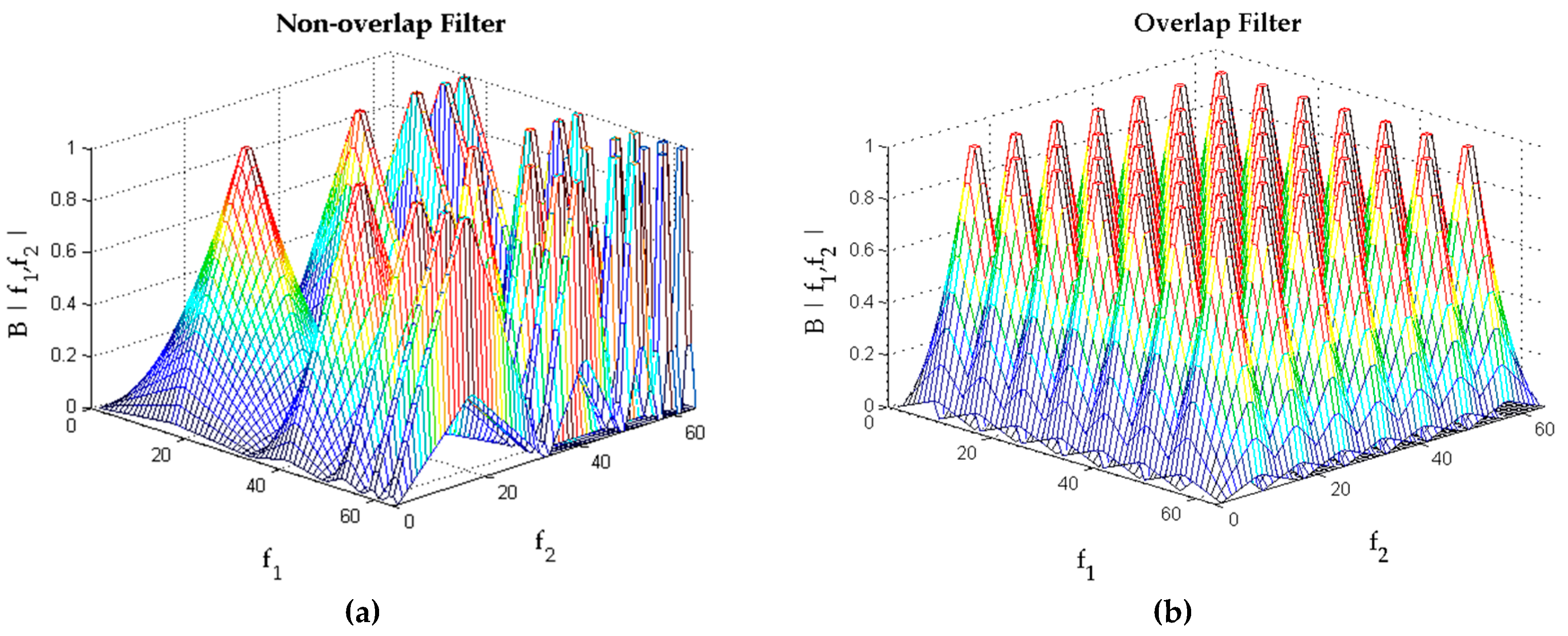
To find the best filtering mechanism, two filter models are proposed, as shown in Figure 3: the non-overlapping filters with various sizes at the base and the overlapping filters with equal sizes at the base. Figure 2b shows that the bispectrum usually gathers near the center; thus, in this area, the filters are dense and the bases are small. At the higher frequencies, the bispectrum usually has a very low value, so in this area, the filters are sparse, and the bases are large. Therefore, in the non-overlapping filters, we use 5 × 5 filters (Figure 3a), with the size of the filter varying (32, 16, 8, 4 and 4) along the x- and y-axis.

By increasing the number of filters and overlapping the filters, the quantization process is expected to provide a better approximation; we therefore increased the number of filters up to 7 × 7 and constructed the filters with overlapping areas at the base (Figure 3b). The size of the bases is 16 × 16 equal elements, and there are 50% overlapping areas with the adjacent filters. However, the complexity and the resulting feature vector’s size of the 7 × 7 filter should be considered as a trade-off.

The height of the overlapping and non-overlapping filters in both pyramid models is equal: in this case, it is one. To filter the bispectrum matrix, each selected area was multiplied by the corresponding filter. The filtering process results in several filtered matrices with their respective bispectrum values, and from these filtered bispectrum matrices, the features are calculated and extracted. The pseudocode of the filtering mechanism for the bispectrum matrices is summarized in Algorithm 2 as follows:

Algorithm 2: Bispectrum 3D filtering for feature extraction algorithm.

Define: M = number of column filter    N = number of row filter  For channel = 1 to C   for m = 1 to M   for n = 1 to N     Calculate length of rectangle base of the filter     Calculate width of rectangle base of the filter     Construct 2D filter for length side of rectangle with triangle type     Construct 2D filter for width side of rectangle with triangle type     Construct 3D pyramid filter based on 2D filter    Take bispectrum value with the length and width of the rectangle     Multiply bispectrum value with the 3D filter    Perform calculation for feature     Take only half of the triangle (non-redundant) of the feature matrix     Transform feature matrix to feature vector    end   end  end

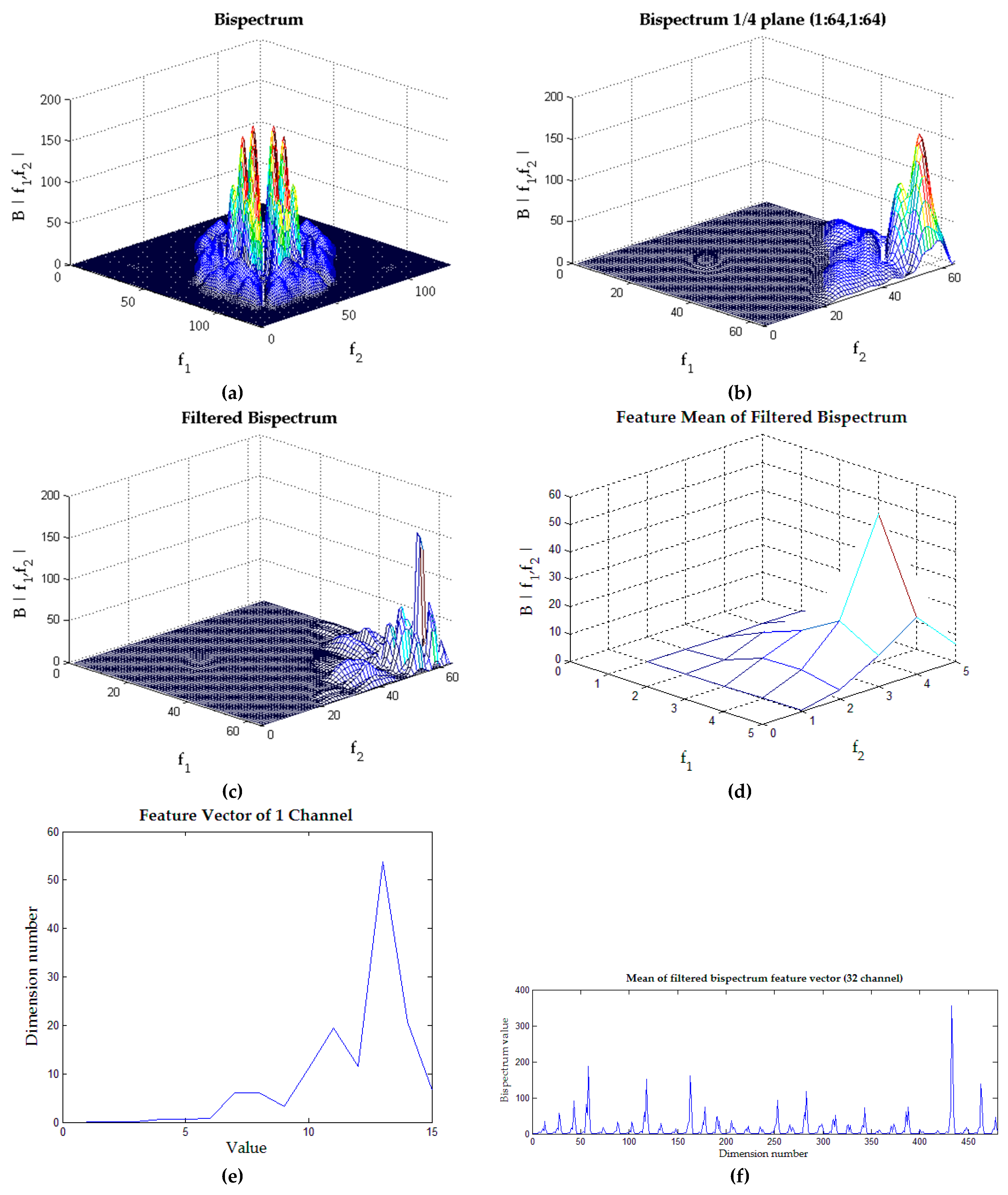
The implementation of the filtering process using the 3D pyramid filters is illustrated in Figure 4. In this example, the effect of 3D pyramid filtering on the bispectrum matrix from the EEG signal of Person 1-Video 1-Channel 1 is shown. The original bispectrum matrix is shown in Figure 4a, and then, one-quarter is extracted, resulting in the 64 × 64 matrix shown in Figure 4b. The filtering process began by multiplying this matrix with the constructed 3D pyramid filters, and for this example, we use the 5 × 5 non-overlapping filters (Figure 3a). The multiplication process was conducted for each area of the matrix according to the size of the pyramid base; for example, the bispectrum matrix region (0:32,0:32) was multiplied by the filter whose base size is 32 × 32 and whose height is one. Therefore, for 5 × 5 non-overlapping filters, there will be 25 times the filtering process through this multiplication step, and the result is shown in Figure 4c. The calculation of features from the filtered bispectrum matrix is then conducted; in this example, the features are the mean (average) of each filtered bispectrum matrix, and the result is shown in Figure 4d.

As the bispectrum matrix shown in Figure 4b is asymmetrical, then the feature-extracted matrix (such as in Figure 4d) is also asymmetrical; therefore, it is sufficient to take just half of the whole matrix. For example, in the 5 × 5 filters, the number of non-redundant elements of the matrix equal to the sum of arithmetic sequence ${{\displaystyle \sum }}_{n=1}^{5}n=15$, resulting in 15 dimensions of feature vectors, as shown in Figure 4e. Thus, for the full 32 EEG channels used, the dimension of feature vectors will be 15 × 32 = 480, as shown in Figure 4f. Obviously, for the 7 × 7 filters, there will be 28 dimensions of feature vector per channel, resulting in 28 × 32 = 896 dimensions of feature vectors for the whole channel.

3.4.3. Feature Types Based on the Bispectrum

Bispectrum analysis has also been used for an EEG-based emotion recognition system by Kumar [20], with several entropies, values and moments taken as the features, which we adapted as one of the feature extraction modes in our experiments (Mode #1 feature extraction); however, this feature produces a high dimension of feature vectors and thus requires a high computation cost. In this work, we propose as simpler feature, which is the mean of the bispectrum value, as Mode #3 feature extraction, producing only one feature value for each area of the filter, thereby reducing the dimension of the feature vectors.

In previous work, we have found that the energy percentage performed well as the feature of an EEG signal [49]; therefore, here, we considered the percentage value as the feature. The percentage value of entropies and moments of Mode #1 becomes the Mode #2 feature extraction, and the percentage of the mean becomes Mode #4 feature extraction. Suppose F_m is a feature and M is the number of features per channel; then, the percentage value of the feature FP_m is defined as:

$$F{P}_m=\frac{F_m}{{{\displaystyle \sum }}_{m=1}^M{F}_m}\times 100.$$

(5)

3.5. Back-Propagation Neural Networks

BPNN is one of the ANN classifiers constructed by the multi-layer perceptron (MLP) architecture. BPNN provides a mechanism to update the weights and biases of each neuron’s connection by propagating and minimizing the error in each iteration (epoch). The BPNN used in this work has three layers of architecture: one input layer, one hidden layer and one output layer. The number of neurons in the input layer was equal to the dimension of the feature vector, while the number of hidden neurons amounted to half of the input neurons. Because the classification for arousal and valence were conducted separately, each emotion was divided into high and low class, resulting in only one neuron in the output layer. The Nguyen–Widrow method [22] was used to initialize the weight and bias of each neuron.

At the feed-forward part of the training phase, for each epoch, the input vectors were presented one at a time to the input layer, and their values were passed to the hidden layer. In the hidden layer, the value received by each neuron was multiplied by its weight and added with the bias. The activation function used was a sigmoid function, f(x) = 1/(1–e^x). On the output layer, the value received by the neuron was multiplied by its weight and added with the bias. The activation function at the output layer was also a sigmoid function, resulting in the output value of the ANN.

At the back-propagation part of the algorithm, the calculated error between the values in the output layer (the predicted emotion) and the target (the actual emotion) was propagated back to adjust the weights and the biases for the neurons in the output and the hidden layer [23]. The learning process was carried on until the preferred minimum error was achieved; in this case, we used root mean sum squared error (RMSSE), or until it reached the maximum number of epochs.

At the testing stage, the testing data part was fed-forward to the input layer and sent to the hidden layer and up to the output layer using the weights and the biases calculated and obtained from the learning stage. The testing stage was similar to the feed-forward part of the learning stage, but the error between the predicted emotion and the stimulated emotion was calculated to produce the recognition rate of the automatic emotion recognition system.

3.6. Probabilistic Neural Networks

PNN is an ANN classifier that is based on Bayes theorem. With a Bayes classifier, the datum X belongs to the class C_j when P(C_j|X) has the biggest probability value.

$$P(C_j|X)=\frac{P(X|C_j)P(C_j)}{P(X)}$$

(6)

To calculate the probability P(C_j|X), it is necessary to estimate the conditional probability P(X|C_j) and the a priori probability of P(C_j) of each class Cj. The calculation of P(X) is not required because P(X) exists in every class. The a priori probability P(C_j) could be calculated by including the entire training data. The conditional probability P(X|C_j) is estimated using the Parzen window p.d.f. estimation. By assuming Gaussian distribution, the Parzen window p.d.f. estimates p_j(x) as:

$$p_j(x)=\frac{1}{\mathrm{N}}{\displaystyle \sum _{\mathrm{k}=1}^{\mathrm{N}}\frac{1}{{(\sigma \sqrt{2\pi })}^d}}{\mathrm{e}}^{(-\frac{1}{2}{(\frac{x-x_{jk}}{\sigma })}^2)}$$

(7)

Here, x is the sample data with the probability being estimated, j is the class number, N is the number of training data in class Cj and d is the dimension of the feature vector. The value of σ (sigma) in the Gaussian distribution is the standard deviation or the smoothing parameter of the Gaussian curve; however, the actual standard distribution was unknown and should be determined.

The PNN consists of four layers: an input layer, a pattern layer, a summation layer and a decision layer. In the input layer, which consists of one neuron, the input vector was received and then forwarded to the pattern layer. Each neuron at the pattern layer represents the training data that belong to each class. We used 50% of the data samples as the training data. Thus, the number of neurons in the pattern layer was equal to 50% of the number of data samples. In the pattern layer, the vector input was compared to the training data in each class. In the summation layer, the Parzen window p.d.f. formula was used to determine the class of the data. The biggest probability value determined where the datum should belong.

4. Experiment and Results

The development of an automatic emotion recognition system using a new methodology for 3D filtered bispectrum feature extraction and the ANN classifier has been presented in Section 3; to verify the performance of the proposed methodology, five experiments were carried out (Exp. #1–Exp. #5). In Exp. #1, to find the best feature extraction type based on bispectrum analysis, four feature extraction types were compared. In Exp. #2, two types of 3D pyramid filters were compared, namely the overlap and the non-overlapping filters. To reduce the computation cost, in Exp. #3, the number of EEG channels used in the system was reduced. In Exp. #4, to increase the recognition rate, the number of samples in the training data was increased to 90%. In the final experiment, Exp. #5, two types of ANN classifiers were compared, the BPNN and the PNN, in order to find the best classifier.

The DEAP database [4] provides EEG signals from 32 people and 40 video stimuli, forming 1280 person-video samples. Originally, the DEAP database used four emotion classes, which are the HAHV (Class 1), the LAHV (Class 2), the LALV (Class 3) and the HALV (Class 4) emotions, by way of H = high, L = low, A = arousal and V = valence, with a balanced sample size (320 samples) resulting from 32 people and 10 video stimuli per class. As indicated in the data acquisition section, this research principally takes two binary classes of emotion in 2D arousal and valence planes: high arousal (Class 1 + Class 4)/low arousal (Class 2 + Class 3) and high valence (Class 1 + Class 2)/low valence (Class 3 + Class 4), with 640 samples for each class, accordingly.

In the following experiments (apart from Exp. #4), 50% of the samples were used as the training data, while the remaining data were used as the testing data, producing 320 samples per class for each of the training and testing parts. All thirty-two people were represented in the training data, but the video stimuli were presented to only a half. For instance, Videos 1–5 (from Class 1) and Videos 31–35 (from Class 4) were chosen as high arousal training data, while Videos 6–10 (from Class 1) and Videos 36–40 (from Class 4) were chosen as testing data. Similarly, Videos 11–15 (from Class 2) and Videos 21–25 (from Class 3) were chosen as low arousal training data, and Videos 16–20 (from Class 2) and Videos 26–30 (from Class 3) were chosen as testing data.

For Exp. #1–Exp. #4, BPNNs were used as the benchmark classifier, with the setting parameters of α (learning rate) = 0.2 and β (momentum) = 0.3. The number of input neurons was equal to the dimension of the feature vectors, the number of hidden neurons is equal to half of the input neurons, and the output of the neurons equals one. In Exp. #5, the PNN was compared with the results of the benchmark classifier.

4.1. Exp. #1: Comparison of Bispectrum-Based Feature Extraction Modes

The following experiments in Exp. #1 were carried out to compare and select the best feature extraction mode from the bispectrum value. There were four types of features to consider: the entropy and moment (NBE, NBSE, MMOB, FOSM and SOSM as in [20]) with additional standard deviation (STD) value as Mode #1, the percentage value of Mode #1 as Mode #2, the mean as Mode #3 and the percentage of the mean as Mode #4. A 5 × 5 3D pyramid filter was used in this experiment, producing 480 dimensions of feature vectors for Mode #3 and Mode #4. The dimensions of feature vectors for Mode #1 and Mode #2 are 2880 because there are six features from each area of the filters (480 × 6 = 2880). To reduce the large dimension, each feature vector was dimensionally reduced using PCA with 99% Eigen values. The comparison result of the feature extraction type Mode #1–Mode #4 is presented in

Table 1. Recognition rate comparison of various feature type. MMOB, mean-magnitude of bispectrum; FOSM, first order spectral moment; SOSM, second order spectral moment; STD, standard deviation.

Feature Type	Features	Maximum Recognition Rate 1		Mean ± SD Recognition Rate
		Arousal (%)	Valence (%)	Arousal (%)	Valence (%)
Mode #1	NBE, NBSE, MMOB, FOSM, SOSM [20], STD	73.36	74.77	64.88 ± 5.32	69.36 ± 5.98
Mode #2	NBE%, NBSE%, MMOB%, FOSM%, SOSM%, STD%	55.24	56.72	54.70 ± 0.41	56.23 ± 0.79
Mode #3	Mean	67.27	71.80	56.11 ± 1.97	54.91 ± 0.96
Mode #4	Mean%	74.22	77.58	72.83 ± 4.04	70.95 ± 9.86

¹ Shown is the maximum recognition rate from 5 repeated experiments.

.

Table 1 shows that the mean percentage feature (Mode #4) provides the highest recognition rate (74.22%) for the arousal and 77.58% for the valence. From the recognition rate in Table 1, it can be seen that for both arousal and valence emotion, Mode #1 and Mode #4 gave the best recognition rate compared to Mode #2 and Mode #3, with Mode #4 providing a slightly better recognition rate than Mode #1. To investigate whether any of the feature types is significantly different, one-way ANOVA was used to compare the recognition rate of four feature type (Mode #1–Mode #4), and the resultant p-values of both separate and combined arousal and valence were all <10⁻⁴. This result suggests Tukey’s HSD test to see which of the feature types is significantly different.

Table 2. Result of statistical significance of Tukey–Kramer HSD test in the arousal and valence recognition rate.

Pairwise Comparison	Arousal			Valence
	Q-Statistic	p-Value	Inference	Q-Statistic	p-Value	Inference
Mode #1 vs. Mode #2	4.611	0.0015	p < 0.05	3.578	0.0121	p < 0.05
Mode #1 vs. Mode #3	3.973	0.0054	p < 0.05	3.940	0.0058	p < 0.05
Mode #1 vs. Mode #4	3.605	0.0114	p < 0.05	0.434	0.9716	p > 0.05
Mode #2 vs. Mode #3	0.6375	0.9183	p > 0.05	0.3620	0.9832	p > 0.05
Mode #2 vs. Mode #4	8.2161	0.0000	p < 0.05	4.0122	0.0050	p < 0.05
Mode #3 vs. Mode #4	7.579	0.0000	p < 0.05	4.374	0.0024	p < 0.05

presents the Tukey HSD test result for pair-wise comparisons. For arousal emotion, Mode #1 is statistically different from Mode #4 with the p-value = 0.0114 (p < 0.05); while for valence emotion, Mode #1 did not have significant difference with Mode #4 with the p-value = 0.9716 (p > 0.05). Moreover, Mode #4 also has shortcomings due to the more complicated feature calculation compared to Mode #1. From this result, we can conclude that for the arousal emotion, the mean percentage of the bispectrum (Mode #4) is a better feature type than entropy and moment (Mode #4), while for the valence emotion, both Mode #1 and Mode #4 are similar. However, it can be noted that both Mode #1 and Mode #4 are significantly different with Mode #2 and Mode #3 (p < 0.05). This experiment also confirmed our hypothesis that the mean percentage of the bispectrum (Mode #4) provides more accurate information than the absolute mean value (Mode #3). This finding implies that for the same emotion, the relative/percentage bispectrum values from the EEG signals may have similarities among people, although different people may have different amplitude in the bispectrum values.

4.2. Exp. #2: Comparison of Overlapped and Non-Overlapped Filters

The newly-developed methodology proposed in this paper is the use of bispectrum analysis and a 3D pyramid filtering for the feature extraction subsystem. The idea of using a 3D pyramid filter as the filtering method is to emphasize the values in the center of the filter and devote less attention to the values at the edges. As Table 1 shows, the mean percentage (Mode #4) with 5 × 5 non-overlapping filters provides a good recognition rate. To improve the recognition rate, the number of filters used for feature extraction was increased to 7 × 7 filters with overlapping filters at the base of the pyramid model. The hypothesis is that by using overlapping filters, the values at the edge of the filters, which have less importance in one filter, will be given higher importance in the adjacent filters; therefore, it is expected that every element of the bispectrum matrix has equal importance. In this experiment we assessed whether the increasing number of the filter will increase the recognition rate. However, we only compare the 5 × 5 filters with the 7 × 7 filters as the first step, and if the higher number of filters results in a higher recognition rate, then the number of filters could be increased more.

In this experiment, we only used the mean percentage feature (Mode #4), following our findings in the previous experiment. Each feature type is dimensionally reduced using PCA with 99% Eigen values. The BPNN was used as the benchmark classifier, and the recognition rate result is presented in

Table 3. Recognition rate results from different filter types.

Filter Type	Maximum Recognition Rate 1		Mean ± SD Recognition Rate
	Arousal (%)	Valence (%)	Arousal (%)	Valence (%)
5 × 5 non-overlapping filters	74.22	77.58	72.83 ± 4.04	70.95 ± 9.86
7 × 7 overlapping filters	64.22	73.13	61.14 ± 3.18	72.81 ± 0.62

¹ Shown is the maximum recognition rate from 5 repeated experiments.

.

Table 3 shows that the 5 × 5 non-overlapping filters gave a higher recognition rate than that of the 7 × 7 overlapping filters, which deviates from our hypothesis. The superiority of the 5 × 5 non-overlapping filters is obvious for the arousal emotion, with a difference up to 10%. One-way ANOVA was used to compare the recognition rate of using the different filter types in the feature extraction process (5 × 5 non-overlapping filters and 7 × 7 overlapping filters). The resultant p-value of the combined arousal and valence emotion recognition rate was p = 0.126 (p > 0.05), which implies that neither of the filter types were significantly different. However, the p-value for arousal emotion recognition rate was p = 0.001 (p < 0.05), and the valence emotion recognition rate was p = 0.685 (p > 0.05). The p-value implies that for the arousal emotion, the use of the 5 × 5 non-overlapping filter was better than the 7 × 7 overlapping filters; however, for the valence emotion, these filters did not differ significantly.

The finding of this Exp. #2 deviated from our hypothesis that increasing the number of filters and by using overlapping strategies in the adjacent filters would increase the recognition rate. The analysis is as follows. The more filters used in the feature extraction process, the higher the dimension of feature vectors produced. However, a higher dimension of feature vectors produces higher cumulative errors, resulting in lower recognition rates. Another reason might be that in the 5 × 5 non-overlapping filters, more attention (by using more numbers and smaller filters) is given to the area where the bispectrum matrix elements show high amplitudes, whereas in the 7 × 7 overlapping filters, all elements of the bispectrum matrix have the same significance. This finding implies that the higher amplitude areas of the bispectrum matrix are more important than the lower ones. Further optimization of the filter type should be investigated as future work, such as by using more numbers of filters, but the size of the filters should be different, which is smaller at the area where the bispectrum amplitudes are high.

4.3. Exp. #3: Channel Selection for Emotion Classification

Research has shown that emotions, and their related brain signals, are associated with the frontal lobe of the cerebral cortex; therefore, the frontal EEG electrodes were often used in the emotion classification research. In this experiment, the effect of channel selection on the recognition rate of the emotion classification system is assessed. The selection of eight and 14 channels is in accordance with our previous work [3]. The reduced eight channels were selected because they are positioned on the frontal and the near frontal area of the cerebral cortex (frontal parietal and anterior-frontal), while the reduced 14 channels were chosen in accordance with the channels available in the BCI Emotiv device. The channel descriptions and the results of this experiment are depicted in

Table 4. Channel selection and description.

∑ Channel	Channel Name	Description	Maximum Recognition Rate 1		Mean ± SD Recognition Rate
			Arousal (%)	Valence (%)	Arousal (%)	Valence (%)
8	F3, F4, F7, F8, Fp1, Fp2, AF3, AF4	Frontal + Frontal Parietal + Anterior-Frontal	74.45	74.06	73.38 ± 1.93	73.52 ± 1.13
14	AF3, F3, F7, FC5, T7, P7, O1, AF4, F4, F8, FC6, T8, P8, O2	BCI channel	75.94	76.02	74.81 ± 0.71	75.00 ± 0.82
32	all channels	DEAP EEG channel	74.22	77.58	72.83 ± 4.04	70.95 ± 9.86

¹ Shown is the maximum recognition rate from 5 repeated experiments.

. BPNN was used for the classifier, and the experiment was repeated five times.

Table 4 shows the recognition rate of the reduced eight and 14 channels compared to the recognition rate of the full 32 channels. One-way ANOVA was used to compare the recognition rate of using the complete and the reduced number of EEG channels. The p-value of the combined arousal and valence recognition rate was p = 0.3 (p > 0.05), while for the arousal emotion recognition rate, p = 0.485 (p > 0.05), and for the valence emotion recognition rate, p = 0.548 (p > 0.05); this finding shows that the reduced eight and 14 channels did not significantly differ from that of the complete 32 channels. This experiment showed that the 14 channels in the BCI equipment are sufficient to conduct emotion classification, with only slight differences compared to that of the 32 EEG channels. However, this experiment ignored the possibility that the signal quality of the BCI equipment might be lower than that of the medical-grade EEG. This experiment also shows that when the research calls for fewer electrodes to reduce the complexity and computation cost, the use of eight electrodes from the frontal, frontal parietal and anterior-frontal regions would be sufficient.

4.4. Exp. #4: Comparison of the Number of Training Samples

To increase the recognition rate, the number of samples in the training data in this experiment was increased to 90%. In the previous experiments (Exp. #1–Exp. #4), the training data composed 50% of the whole dataset, and all samples in the dataset were used for testing. In this experiment, the amount of training data samples was increased to 90% of all data samples, and classification was conducted using a 10-fold cross-validation method. There were 1152 samples used for the training data out of the 1280 samples available in the dataset. The division of the 10-fold cross-validation was designed so that if any of the video stimuli produced a different emotion from the emotion class desired, then it would be depicted in the recognition result. Therefore, for Fold 1 (F1), the sample data from the people with Videos 1, 11, 21 and 31 were used as testing data, while the rest was used for training. Similarly, for Fold 2 (F2), sample data from the people with Videos 2, 12, 22 and 32 were used for testing, and the rest were used for training, and so on, until Fold 10 (F10). This experiment was conducted using a BPNN classifier, and the reduced eight channels were used as the input.

From the data shown in

Table 5. Result of the 10-fold cross-validation recognition rate for mean percentage feature type from 8 EEG channels with 5 × 5 non-overlapped filters.

Emotion Type	F1 (%)	F2 (%)	F3 (%)	F4 (%)	F5 (%)	F6 (%)	F7 (%)	F8 (%)	F9 (%)	F10 (%)	Mean (%)
Arousal	92.66	92.50	92.42	93.13	93.98	93.44	92.50	93.44	92.66	92.11	92.92
Valence	93.44	93.13	93.59	93.52	93.83	93.20	93.59	93.98	93.44	93.28	93.51
Arousal (LSO)	54.69	51.56	50.00	57.03	57.03	53.13	55.47	51.56	54.69	47.66	53.28
Valence (LSO)	55.47	59.38	55.47	57.03	51.56	60.16	60.16	58.59	55.47	58.59	57.19

it can be seen that the recognition rate results from the 10-fold cross-validation are 92.92% for arousal and 93.51% for valence. One-way ANOVA resulted in the p-value = 0.669 (p > 0.05); thus, there is no significant difference between the fold. This experiment implies that by increasing the training data up to 90%, the recognition rate increased by an average of 18.96% (18.47% and 19.42% for arousal and valence), and the comparison of recognition rates between using 50% training data and 90% training data is depicted in Figure 5. From this result, it can be concluded that the amount of training data greatly influences the results obtained, and the higher the ratio of the training data, the higher the recognition rate.

In a leave subject out (LSO) training-testing method, each fold in this experiment represented the video used as the stimulus as the subject, instead of the person. The recognition rate for the arousal emotion was on average 53.28% and for the valence emotion was 57.19%. This finding was comparable to recent other research results using the same database, such as the leave-subject-out scheme of the person (53.42% for arousal and 52.05% for valence) [37], using a random subset 10-fold leave-p-out cross-validation (all between 40% and 50% accuracy) [50].

4.5. Exp. #5: Comparison of BPNN and PNN Classifiers

To find the best classifier for the automatic emotion recognition system, two types of ANN classifiers were compared, the BPNN and the PNN. The drawback of the BPNN was the computing time to conduct the training phase for the classifier; thus, the PNN, which is generally faster than the BPNN, was used in this experiment.

The BPNN setting parameter was similar to that of the previous experiments (Exp. #1–Exp. #4), whereas for the PNN, it is difficult to find a good choice of smoothing parameter (σ), because in the original PNN classifier, there is no mathematical calculation to determine the best smoothing parameter. In this experiment, the PNN smoothing parameter (σ) was chosen randomly, and the trial was repeated 60 times to find the highest recognition rate. In this experiment, we used only eight channels from the EEG signals, as the previous experiment showed that using eight channels would be sufficient. The PNN recognition result for various randomly-generated smoothing parameters (σ) can be seen in Figure 6.

From the randomly-generated smoothing parameter (σ), we could find the optimum PNN recognition rate, which is 76.09% when σ = 0.4505 for arousal and 75.31% when σ = 0.3517 for valence, as depicted in Figure 6. The comparison of the recognition rate and the computing time between the PNN and the BPNN is presented in

Table 6. Comparison of results from BPNN and PNN.

	ANN Type	Time (s)	Recognition Rate (%)	Sensitivity	Specificity	PPV
Arousal	BPNN	448.35	74.45	0.74	0.75	0.75
	PNN	2.09	76.09	0.89	0.63	0.71
Valence	BPNN	448.21	74.06	0.75	0.74	0.74
	PNN	2.09	75.31	0.93	0.58	0.69

.

From Table 6, we can see that the recognition rate from both the BPNN and the PNN for arousal and valence emotion was comparable, with both values hovering around 75%, with the p-value of 0.761 (p > 0.05). However, the specificity of PNN is lower than BPNN, and the sensitivity was higher than BPNN, meaning that PNN detected more positive values (the higher emotion level) compared to BPNN, but PNN has a lower ability to detect the negative values (the lower emotion level) compared to BPNN. As for the positive predictive value (PPV) value, it can be seen that both classifiers are comparable with a slightly higher value of PPV from BPNN. If PPV is used as the “gold standard” as mentioned by Parikh [51], then BPNN is superior to PNN in classifying emotion from EEG signals.

As depicted in the receiver operating characteristics (ROC) graph in Figure 7, the BPNN is more “conservative” than the PNN because for both emotion, i.e., the arousal and the valence, the BPNN position is on the left side of the PNN. From this ROC analysis, it can be stated that BPNN makes positive classifications with strong evidence, so it makes few false positive errors. According to Fawcett [52], in a real-word classification problem, there are more negative instance than the positive ones; thus, the far-left handed side of the ROC graph becomes more interesting; thus, from this point of view, the BPNN performed better than the PNN.

Although the maximum value achieved was not significantly different, the computing time of the PNN for a single run was about 200-times faster than that of the BPNN. However, PNN requires an optimization method for finding the best sigma value, whereas the BPNN does not require prior optimization; thus, the iterative training for BPNN can be conducted only once. Nevertheless, for this experiment, the total time for running 60 time trials of PNN is still faster (60 × 2.09 = 125.4 s) compared to a single run of BPNN (448 s), which is about 3.5-times faster. Using one-way ANOVA, the time difference between BPNN and PNN shows a significant difference with p < 10⁻⁴.

5. Discussion and Conclusions

In our developed automatic emotion recognition system, we propose a new methodology for EEG signal feature extraction using bispectrum analysis, a 3D pyramid filtering method and an ANN-based classifier. The proposed method could recognize two binary types of emotion—high/low arousal and high/low valence—from the EEG input signals provided by the DEAP benchmark database. From the feature extraction mode experiment (Exp. #1), the mean percentage of the bispectrum provided the best recognition rate with lower complexity (74.22% for the arousal and 77.58% for the valence). To reduce and extract the features from the bispectrum values, we propose a new method of filtering by means of 3D pyramid filters and by comparing the 5 × 5 non-overlapping and the 7 × 7 overlapping filters (Exp. #2); we found that the 5 × 5 non-overlapping filters with various pyramid base sizes provide the highest recognition rate.

The reduction of channels (Exp. #3) did not significantly affect the recognition rate. Therefore, we conclude that the channels provided in the BCI equipment are sufficient to conduct emotion classification, and when it is more suitable to use fewer electrodes to reduce complexity and computation cost, the choice of eight electrodes in the frontal, frontal parietal and anterior-frontal regions is also sufficient. By increasing the number of training data samples to 90% of the entire dataset (Exp. #4), the recognition rate was increased by 18.96%; from this result, it can be noted that the amount of training data used greatly influences the results obtained. We also compared the benchmark BPNN classifier with a PNN classifier for the eight EEG channels’ input (Exp. #5), and we achieved a slightly better result: 76.09% for arousal and 75.31% for valence. Although the result is not significantly higher, the computing time of the PNN to achieve the maximum recognition rate result is about 3.5-times faster than the BPNN.

The proposed bispectrum-based feature extraction gave a comparable result with some recent research using different feature extraction methods, such as Discrete Wavelet Transform - Relative Wavelet Energy (DWT-RWE) [3], Short Time Fourier Transform (STFT) [50], Power Spectral Density (PSD) [37] and Empirical Mode Decomposition (EMD) with Sample Entropy (SampEn) [53]. Future studies in the EEG-based emotion recognition system should focus on improving the feature calculation from the bispectrum values. This research utilized two non-linear classifiers, namely the BPNN and the PNN. The result of using these classifier was also comparable to other recent research using other linear and non-linear classifier, such as SVM [50,53] and DLN [37]. However, newer classifiers, such as group sparse canonical correlation analysis (GCCA) [54] and sparse deep belief networks (SDBN) [55], have never been used, giving room to further future works.

References

1. Mumford, E.; Schlesinger, H.J.; Glass, G.V. The effects of psychological intervention on recovery from surgery and heart attacks: An analysis of the literature. Am. J. Public Health 1982, 72, 141–151. [Google Scholar] [CrossRef] [PubMed]
2. Kim, M.; Kim, M.; Oh, E.; Kim, S. A Review on the Computational Methods for Emotional State Estimation from the Human EEG. Comput. Math. Methods Med. 2013. [Google Scholar] [CrossRef] [PubMed]
3. Purnamasari, P.D.; Ratna, A.A.P.; Kusumoputro, B. Artificial Neural Networks Based Emotion Classification System through Relative Wavelet Energy of EEG Signal. In Proceedings of the Fifth International Conference on Network, Communication and Computing (ICNCC 2016), Kyoto, Japan, 17–21 December 2016; pp. 135–139. [Google Scholar]
4. Koelstra, S.; Lee, J.; Yazdani, A.; Ebrahimi, T.; Pun, T.; Nijholt, A.; Patras, I. DEAP: A Database for Emotion Analysis Using Physiological Signals. IEEE Trans. Affect. Comput. 2012, 3, 1–15. [Google Scholar] [CrossRef]
5. Jenke, R.; Peer, A.; Buss, M. Feature Extraction and Selection for Emotion Recognition from EEG. IEEE Trans. Affect. Comput. 2014, 5, 327–339. [Google Scholar] [CrossRef]
6. Solomon, B.; DeCicco, J.M.; Dennis, T.A. Emotional picture processing in children: An ERP study. Dev. Cogn. Neurosci. 2012, 2, 110–119. [Google Scholar] [CrossRef] [PubMed]
7. Goyal, M.; Singh, M.; Singh, M. Classification of emotions based on ERP feature extraction. In Proceedings of the 2015 1st International Conference on Next Generation Computing Technologies (NGCT), Dehradun, India, 4–5 September 2015; pp. 660–662. [Google Scholar]
8. Hajcak, G.; Macnamara, A.; Olvet, D.M. Event-Related Potentials, Emotion, and Emotion Regulation: An Integrative Review. Dev. Neuropsychol. 2010, 32, 129–155. [Google Scholar] [CrossRef] [PubMed]
9. Kaestner, E.J.; Polich, J. Affective recognition memory processing and event-related brain potentials. Cogn. Affect. Behav. Neurosci. 2011, 11, 186–198. [Google Scholar] [CrossRef] [PubMed]
10. Bastos-Filho, T.F.; Ferreira, A.; Atencio, A.C.; Arjunan, S.; Kumar, D. Evaluation of feature extraction techniques in emotional state recognition. In Proceedings of the 2012 4th International Conference on Intelligent Human Computer Interaction: Advancing Technology for Humanity (IHCI), Kharagpur, India, 27–29 December 2012. [Google Scholar]
11. Jatupaiboon, N.; Pan-Ngum, S.; Israsena, P. Real-time EEG-based happiness detection system. Sci. World J. 2013, 2013. [Google Scholar] [CrossRef] [PubMed]
12. Daimi, S.N.; Saha, G. Classification of emotions induced by music videos and correlation with participants’ rating. Expert Syst. Appl. 2014, 41, 6057–6065. [Google Scholar] [CrossRef]
13. Rozgic, V.; Vitaladevuni, S.N.; Prasad, R. Robust EEG emotion classification using segment level decision fusion. In Proceedings of the 2013 IEEE International Conference on Acoustics, Speech and Signal Processing (ICASSP), Vancouver, BC, Canada, 26–31 May 2013; pp. 1286–1290. [Google Scholar]
14. Sigl, J.C.; Chamoun, N.G. An introduction to bispectral analysis for the electroencephalogram. J. Clin. Monit. 1994, 10, 392–404. [Google Scholar] [CrossRef] [PubMed]
15. Miller, A.; Sleigh, J.W.; Barnard, J.; Steyn-Ross, D.A. Does bispectral analysis of the electroencephalogram add anything but complexity? Br. J. Anaesth. 2004, 92, 8–13. [Google Scholar] [CrossRef] [PubMed]
16. Hagihira, S.; Takashina, M.; Mori, T.; Mashimo, T.; Sleigh, J.W.; Barnard, J.; Miller, A.; Steyn-Ross, D.A. Bispectral analysis gives us more information than power spectral-based analysis. Br. J. Anaesth. 2004, 92, 772–773. [Google Scholar] [CrossRef] [PubMed]
17. Goshvarpour, A.; Goshvarpour, A.; Rahati, S. Bispectrum Estimation of Electroencephalogram Signals During Meditation. Iran. J. Psychiatry Behav. Sci. 2012, 6, 48–54. [Google Scholar] [PubMed]
18. Ning, T.; Bronzino, J.D. Bispectral Analysis of the Rat EEG During Various Vigilance States. IEEE Trans. Biomed. Eng. 1989, 36, 1988–1990. [Google Scholar] [CrossRef] [PubMed]
19. Hosseini, S.A.; Khalilzadeh, M.A.; Naghibi-sistani, M.B.; Niazmand, V. Higher Order Spectra Analysis of EEG Signals in Emotional Stress States. In Proceedings of the 2010 2nd International Conference on Information Technology and Computer Science, Kiev, Ukraine, 24–25 July 2010; pp. 60–63. [Google Scholar]
20. Kumar, N.; Khaund, K.; Hazarika, S.M. Bispectral Analysis of EEG for Emotion Recognition. Proced. Comput. Sci. 2016, 84, 31–35. [Google Scholar] [CrossRef]
21. Vijayan, A.E.; Sen, D.; Sudheer, A.P. EEG-Based Emotion Recognition Using Statistical Measures and Auto-Regressive Modeling. In Proceedings of the 2015 IEEE International Conference on Computational Intelligence & Communication Technology (CICT), Ghaziabad, India, 13–14 February 2015; pp. 587–591. [Google Scholar]
22. Gotlib, I.H.H.; Ranganath, C.; Rosenfeld, J.P.P. EEG Alpha Asymmetry, Depression, and Cognitive Functioning. Cogn. Emot. 1998, 12, 449–478. [Google Scholar] [CrossRef]
23. Balconi, M.; Mazza, G. Brain oscillations and BIS/BAS (behavioral inhibition/activation system) effects on processing masked emotional cues. ERS/ERD and coherence measures of alpha band. Int. J. Psychophysiol. 2009, 74, 158–165. [Google Scholar] [CrossRef] [PubMed]
24. Muller, M.M.; Keil, A.; Gruber, T.; Elbert, T. Processing of affective pictures modulates right-hemisphere gamma band activity. Clin. Neurophysiol. 1999, 110, 1913–1920. [Google Scholar] [CrossRef]
25. Balconi, M.; Lucchiari, C. Consciousness and arousal effects on emotional face processing as revealed by brain oscillations. A gamma band analysis. Int. J. Psychophysiol. 2008, 67, 41–46. [Google Scholar] [CrossRef] [PubMed]
26. Aftanas, L.I.; Varlamov, A.A.; Pavlov, S.V.; Makhnev, V.P.; Reva, N.V. Affective picture processing: Event-related synchronization within individually defined human theta band is modulated by valence dimension. Neurosci. Lett. 2001, 303, 115–118. [Google Scholar] [CrossRef]
27. Murugappan, M. Classification of human emotion from EEG using discrete wavelet transform. J. Biomed. Sci. Eng. 2010, 3, 390–396. [Google Scholar] [CrossRef]
28. Li, M.; Lu, B.L. Emotion classification based on gamma-band EEG. In Proceedings of the 2009 31st Annual International Conference of the IEEE Engineering in Medicine and Biology Society: Engineering the Future of Biomedicine (EMBC), Piscataway, NJ, USA, 3–6 September 2009; pp. 1323–1326. [Google Scholar]
29. Lin, Y.P.; Wang, C.H.; Jung, T.P.; Wu, T.L.; Jeng, S.K.; Duann, J.R.; Chen, J.H. EEG-based emotion recognition in music listening. IEEE Trans. Biomed. Eng. 2010, 57, 1798–1806. [Google Scholar] [PubMed]
30. Petrantonakis, P.C.; Hadjileontiadis, L.J. Emotion recognition from EEG using higher order crossings. IEEE Trans. Inf. Technol. Biomed. 2010, 14, 186–197. [Google Scholar] [CrossRef] [PubMed]
31. Wang, X.; Nie, D.; Lu, B. EEG-based emotion recognition using frequency domain features and support vector machines. Neural Inf. Process. 2011, 734–743. [Google Scholar] [CrossRef]
32. Yazdani, A.; Lee, J.-S.; Vesin, J.-M.; Ebrahimi, T. Affect recognition based on physiological changes during the watching of music videos. ACM Trans. Interact. Intell. Syst. 2012, 2, 1–26. [Google Scholar] [CrossRef]
33. Murugappan, M.; Nagarajan, R.; Yaacob, S. Combining spatial filtering and wavelet transform for classifying human emotions using EEG Signals. J. Med. Biol. Eng. 2011, 31, 45–51. [Google Scholar] [CrossRef]
34. Brown, L.; Grundlehner, B.; Penders, J. Towards wireless emotional valence detection from EEG. In Proceedings of the 2011 33rd Annual International Conference of the IEEE Engineering in Medicine and Biology Society (EMBS), Piscataway, NJ, USA, 30 August–3 September 2011; pp. 2188–2191. [Google Scholar]
35. Zhang, J.; Chen, M.; Hu, S. PNN for EEG-based Emotion Recognition. In Proceedings of the 2016 IEEE International Conference on Systems, Man and Cybernetics, Budapest, Hungary, 9–12 October 2016; pp. 2319–2323. [Google Scholar]
36. Chai, R.; Tran, Y.; Naik, G.R.; Nguyen, T.N.; Ling, S.H.; Craig, A.; Nguyen, H.T. Classification of EEG based-mental fatigue using principal component analysis and Bayesian neural network. In Proceedings of the 2016 38th Annual International Conference of the IEEE Engineering in Medicine and Biology Society (EMBC), Orlando, FL, USA, 16–20 August 2016; pp. 4654–4657. [Google Scholar]
37. Jirayucharoensak, S.; Pan-Ngum, S.; Israsena, P. EEG-Based Emotion Recognition Using Deep Learning Network with Principal Component Based Covariate Shift Adaptation. Sci. World J. 2014, 2014. [Google Scholar] [CrossRef] [PubMed]
38. Goldberger, A.L.; Amaral, L.A.N.; Glass, L.; Hausdorff, J.M.; Ivanov, P.C.; Mark, R.G.; Mietus, J.E.; Moody, G.B.; Peng, C.-K.; Stanley, H.E. PhysioBank, PhysioToolkit, and PhysioNet. Circulation 2000, 101, e215–e220. [Google Scholar] [CrossRef] [PubMed]
39. Schalk, G.; McFarland, D.J.; Hinterberger, T.; Birbaumer, N.; Wolpaw, J.R. BCI2000: A General-Purpose Brain-Computer Interface (BCI) System. IEEE Trans. Biomed. Eng. 2004, 51, 1034–1043. [Google Scholar] [CrossRef] [PubMed]
40. Kemp, B.; Zwinderman, A.H.; Tuk, B.; Kamphuisen, H.A.C.; Oberyé, J.J.L. Analysis of a Sleep-Dependent Neuronal Feedback Loop: The Slow-Wave Microcontinuity of the EEG. IEEE Trans. Biomed. Eng. 2000, 47, 1185–1194. [Google Scholar] [CrossRef] [PubMed]
41. Zwoliński, P.; Roszkowski, M.; Zygierewicz, J.; Haufe, S.; Nolte, G.; Durka, P.J. Open database of epileptic EEG with MRI and postoperational assessment of foci—A real world verification for the EEG inverse solutions. Neuroinformatics 2010, 8, 285–299. [Google Scholar] [CrossRef] [PubMed]
42. Soleymani, M.; Lichtenauer, J.; Pun, T.; Pantic, M. A Multimodal Database for Affect Recognition and Implicit Tagging. IEEE Trans. Affect. Comput. 2012, 3, 42–55. [Google Scholar] [CrossRef]
43. Zheng, W.L.; Lu, B.L. Investigating Critical Frequency Bands and Channels for EEG-Based Emotion Recognition with Deep Neural Networks. IEEE Trans. Auton. Ment. Dev. 2015, 7, 162–175. [Google Scholar] [CrossRef]
44. Jadhav, P.N.; Shanamugan, D.; Chourasia, A.; Ghole, A.R.; Acharyya, A.; Naik, G. Automated detection and correction of eye blink and muscular artefacts in EEG signal for analysis of Autism Spectrum Disorder. In Proceedings of the 2014 36th Annual International Conference of the IEEE Engineering in Medicine and Biology Society (EMBC), Chicago, IL, USA, 26–30 August 2014; Volume 2014, pp. 1881–1884. [Google Scholar]
45. Bhardwaj, S.; Jadhav, P.; Adapa, B.; Acharyya, A.; Naik, G.R. Online and automated reliable system design to remove blink and muscle artefact in EEG. In Proceedings of the 2015 37th Annual International Conference of the IEEE Engineering in Medicine and Biology Society (EMBC), Piscataway, NJ, USA, 25–29 August 2015; Volume 2015, pp. 6784–6787. [Google Scholar]
46. Nikias, C.L.; Mendel, J.M. Signal processing with higher-order spectra. IEEE Signal Process. Mag. 1993, 10, 10–37. [Google Scholar] [CrossRef]
47. Kusumoputro, B.; Triyanto, A.; Fanany, M.I.; Jatmiko, W. Speaker identification in noisy environment using bispectrum analysis and probabilistic neural network. In Proceedings of the 4th International Conference on Computational Intelligence and Multimedia Applications (ICCIMA), Yokosuka City, Japan, 30 October–1 November 2001; pp. 282–287. [Google Scholar]
48. Brillinger, D. An introduction to polyspectra. Ann. Math. Stat. 1965, 36, 1351–1374. [Google Scholar] [CrossRef]
49. Purnamasari, P.D.; Ratna, A.A.P.; Kusumoputro, B. EEG Based Patient Emotion Monitoring using Relative Wavelet Energy Feature and Back Propagation Neural Network. In Proceedings of the 2015 37th Annual International Conference of the IEEE Engineering in Medicine and Biology Society (EMBC), Milan, Italy, 25–29 August 2015; pp. 2820–2823. [Google Scholar]
50. Ackermann, P.; Kohlschein, C.; Wehrle, K.; Jeschke, S. EEG-based Automatic Emotion Recognition: Feature Extraction, Selection and Classification Methods. In Proceedings of the 2016 IEEE 18th International Conference on e-Health Networking, Applications and Services (Healthcom), Munich, Germany, 14–16 September 2016. [Google Scholar]
51. Parikh, R.; Mathai, A.; Parikh, S.; Chandra Sekhar, G.; Thomas, R. Understanding and using sensitivity, specificity and predictive values. Indian J. Ophthalmol. 2008, 56, 45–50. [Google Scholar] [CrossRef] [PubMed]
52. Fawcett, T. An introduction to ROC analysis. Pattern Recognit. Lett. 2006, 27, 861–874. [Google Scholar] [CrossRef]
53. Zhang, Y.; Ji, X.; Zhang, S. An approach to EEG-based emotion recognition using combined feature extraction method. Neurosci. Lett. 2016, 633, 152–157. [Google Scholar] [CrossRef] [PubMed]
54. Zheng, W. Multichannel EEG-Based Emotion Recognition via Group Sparse Canonical Correlation Analysis. IEEE Trans. Cogn. Dev. Syst. 2016, 8920. [Google Scholar] [CrossRef]
55. Chai, R.; Ling, S.H.; San, P.P.; Naik, G.R.; Nguyen, T.N.; Tran, Y.; Craig, A.; Nguyen, H.T. Improving EEG-Based Driver Fatigue Classification Using Sparse-Deep Belief Networks. Front. Neurosci. 2017, 11, 103. [Google Scholar] [CrossRef] [PubMed]
Figure 1. Block diagram of the EEG-based emotion recognition system.
Algorithms 10 00063 g001
Figure 2. Comparison between (a) power spectrum which shows dominant frequencies and (b) bispectrum, which shows dominant frequencies and their correlation (if any).
Algorithms 10 00063 g002
Figure 3. Two types of 3D filtering using pyramid models with (a) 5 × 5 non-overlap and (b) 7 × 7 overlapping filters.
Algorithms 10 00063 g003
Figure 4. Bispectrum filtering step: (a) the original bispectrum contour plot, (b) one-quarter of the bispectrum matrix, (c) the result of the filtering process, (d) the mean as the feature, (e) the feature vector constructed from the non-redundant region of the quantized matrix and (f) the full feature vectors from the 32 channels.
Algorithms 10 00063 g004
Figure 5. Recognition rate for different amounts of data training samples.
Algorithms 10 00063 g005
Figure 6. PNN results for various smoothing parameter values for (a) arousal and (b) valence emotion.
Algorithms 10 00063 g006
Figure 7. ROC plot of BPNN and PNN as the classifier.
Algorithms 10 00063 g007