
The Shear Mechanisms of Natural Fractures during the Hydraulic Stimulation of Shale Gas Reservoirs

Abstract
:
1. Introduction
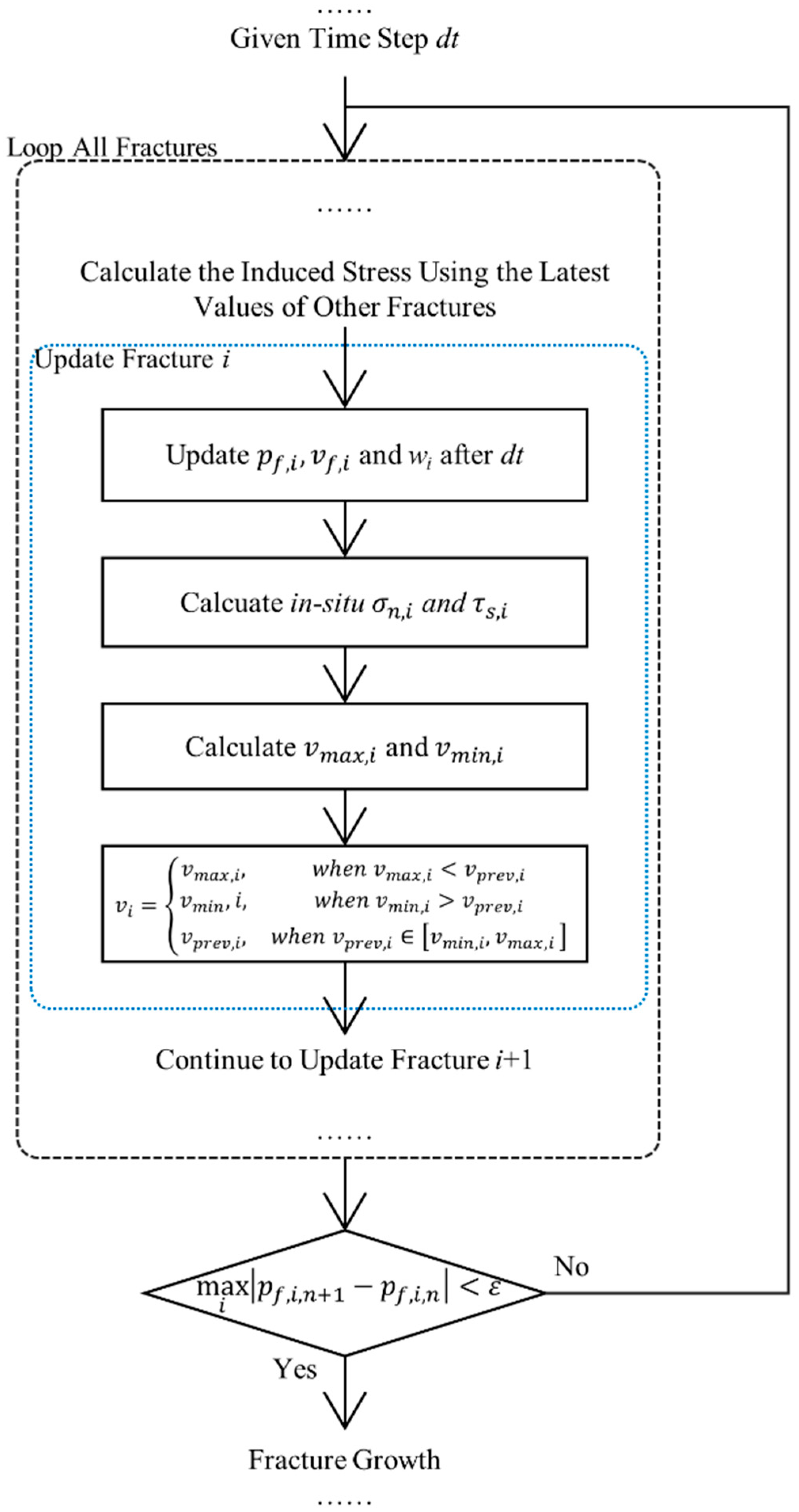
2. Numerical Method
3. Results and Discussion
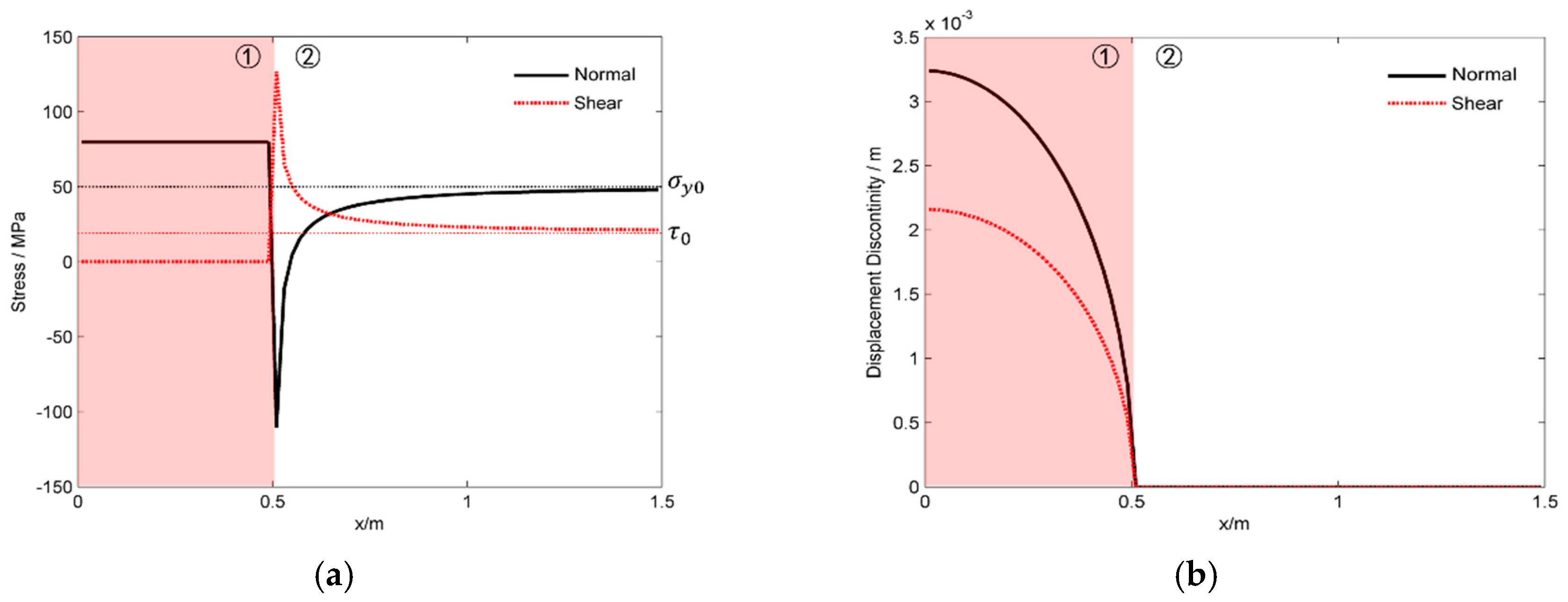
3.1. The Shearing of Single Fracture
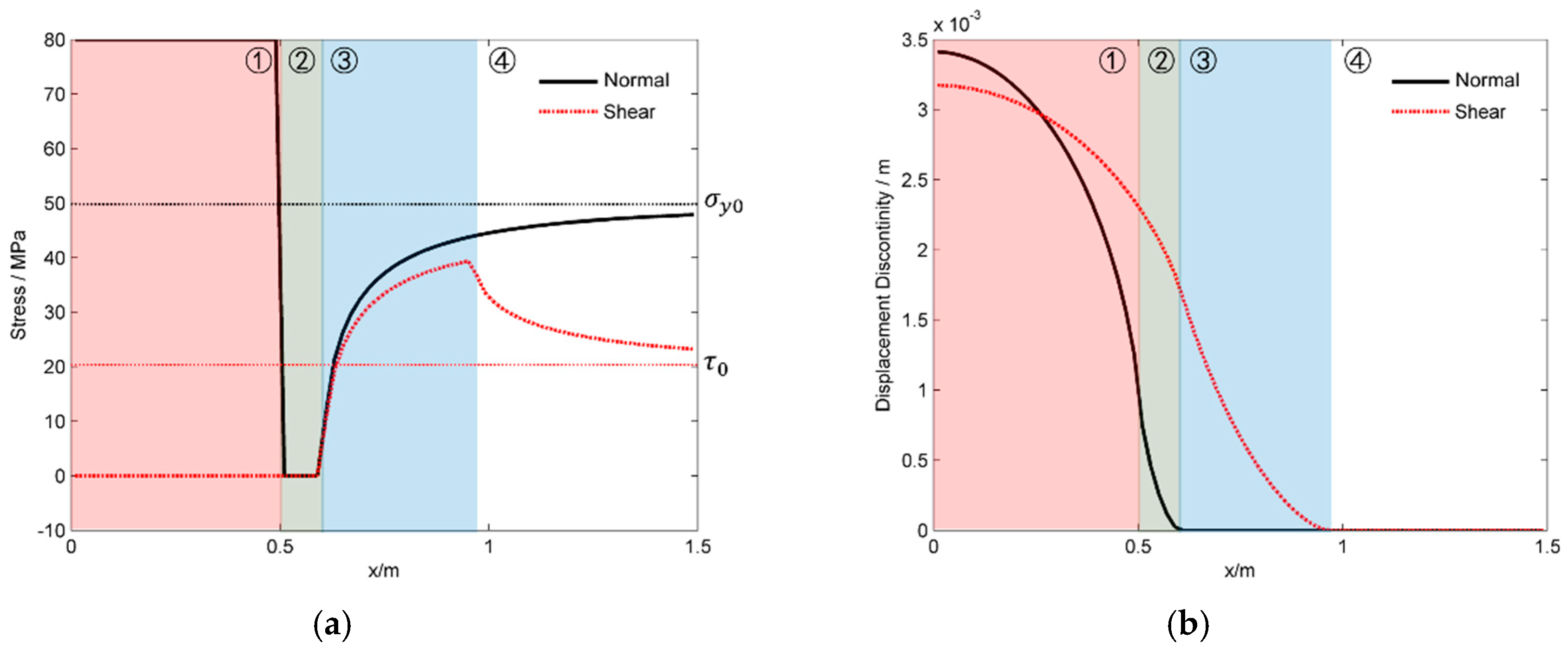
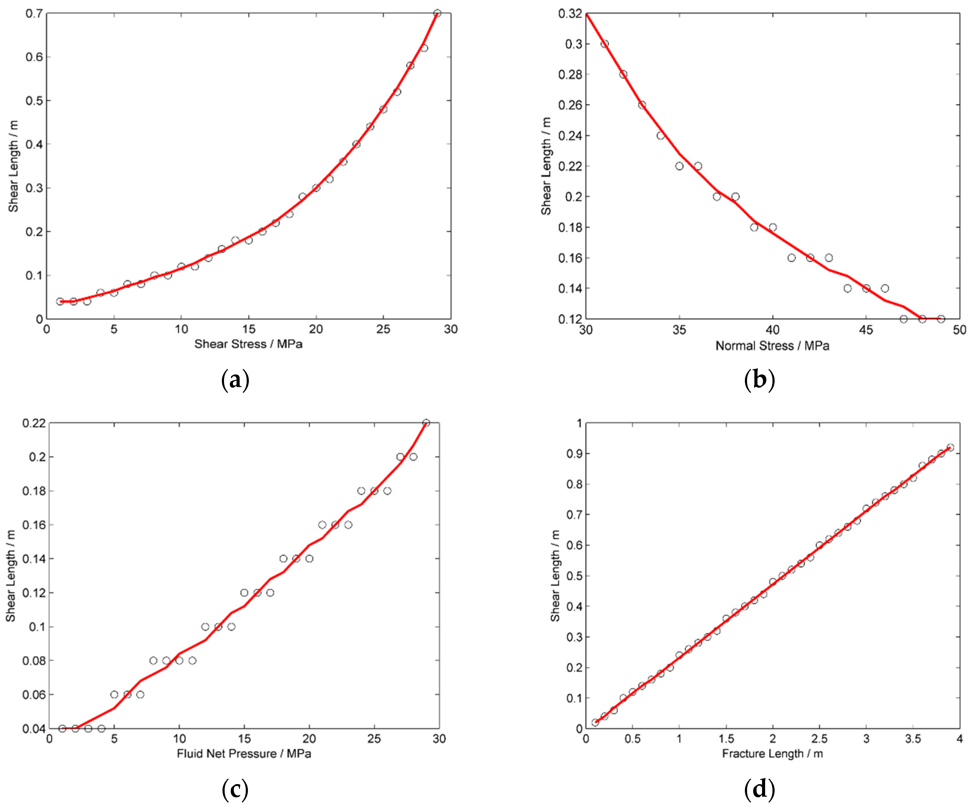
3.2. The Shear Fracture Length
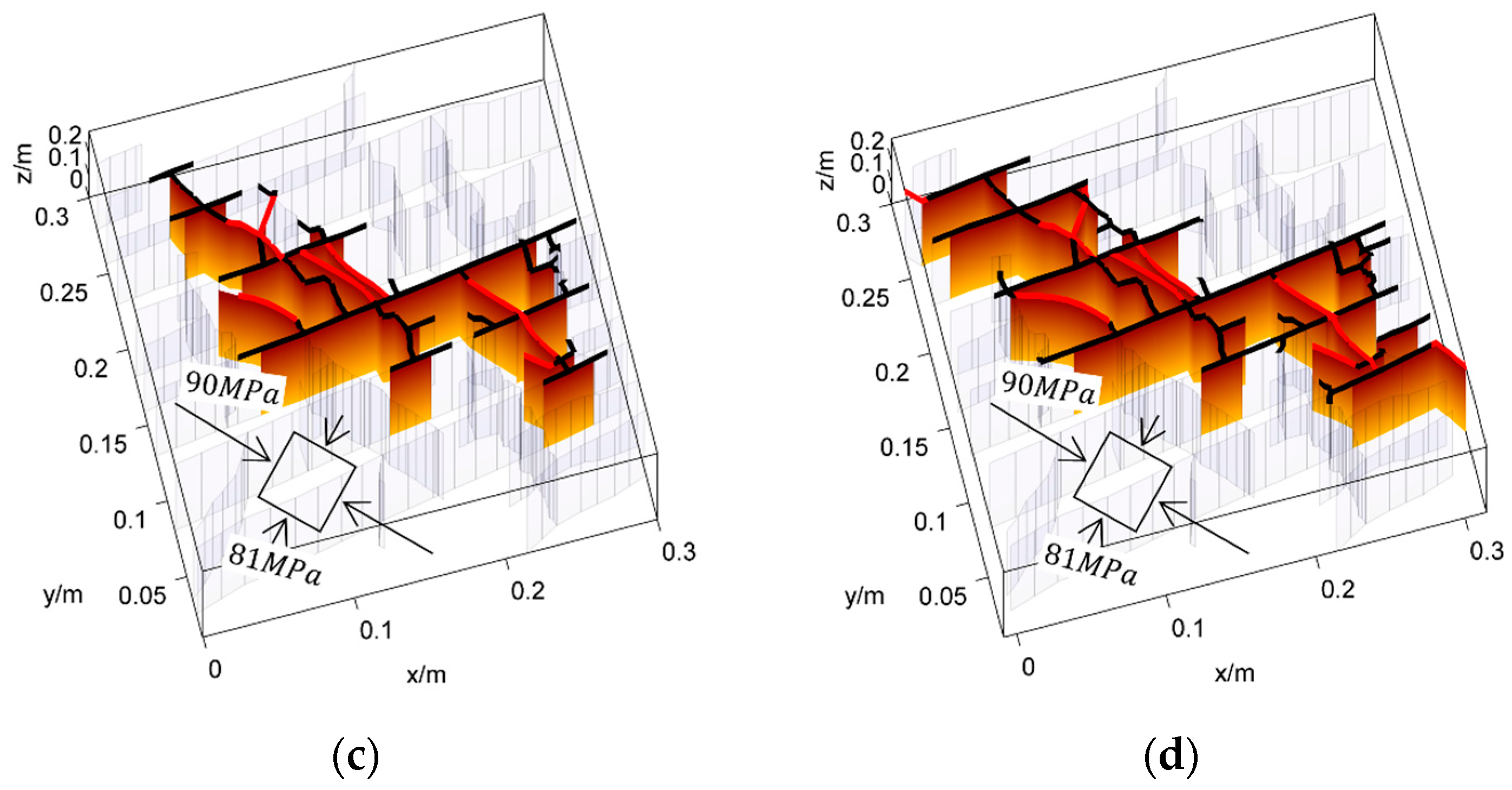
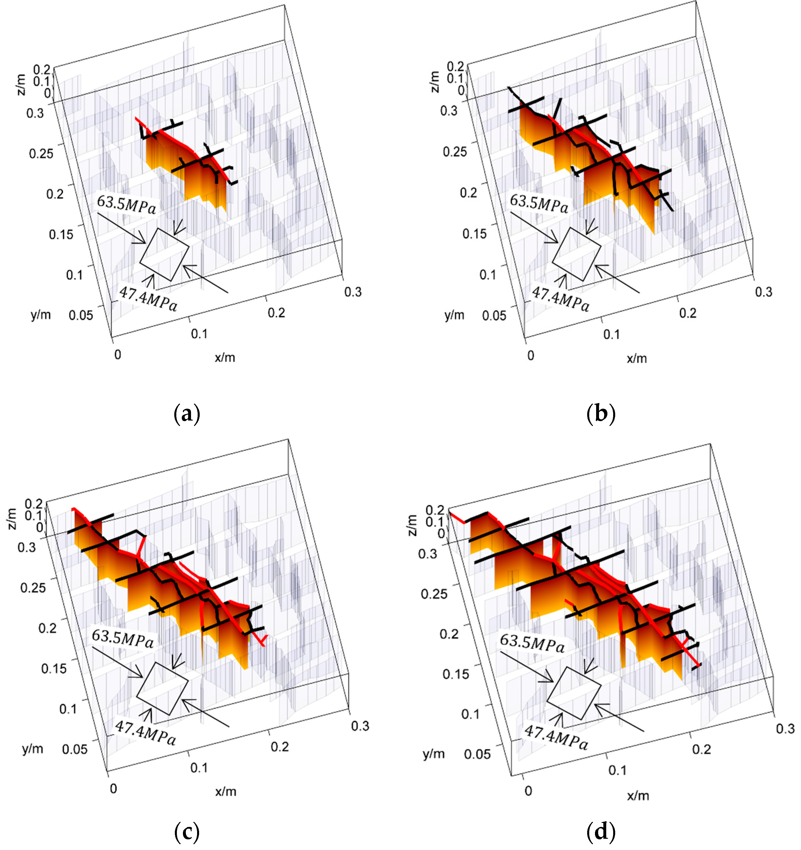
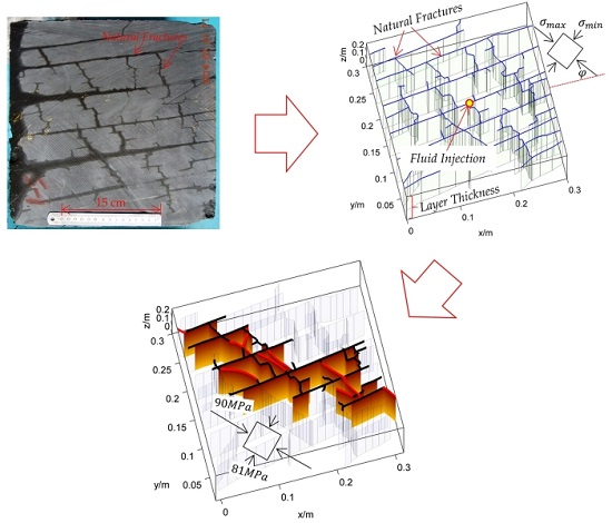
3.3. The Shearing of a Complex Fracture Network
4. Conclusions
Acknowledgments
Author Contributions
Conflicts of Interest
References
- Riahi, A.; Damjanac, B. Numerical study of interaction between hydraulic fracture and discrete fracture network. In Proceedings of the ISRM International Conference for Effective and Sustainable Hydraulic Fracturing, Brisbane, Australia, 20–22 May 2013; International Society for Rock Mechanics: Brisbane, Australia, 2013. [Google Scholar]
- Majer, E.L.; Baria, R.; Stark, M.; Oates, S.; Bommer, J.; Smith, B.; Asanuma, H. Induced seismicity associated with enhanced geothermal systems. Geothermics 2007, 36, 185–222. [Google Scholar] [CrossRef]
- Pine, R.J.; Batchelor, A.S. Downward migration of shearing in jointed rock during hydraulic injections. Int. J. Rock Mech. Min. Sci. 1984, 21, 249–263. [Google Scholar] [CrossRef]
- Zoback, M.D.; Kohli, A.; Das, I.; McClure, M.W. The importance of slow slip on faults during hydraulic fracturing stimulation of shale gas reservoirs. In Proceedings of the Americas Unconventional Resources Conference, Pittsburgh, PA, USA, 5–7 June 2012; Society of Petroleum Engineers: Pittsburgh, PA, USA, 2012. [Google Scholar]
- Zhang, X.; Jeffrey, R.; Llanos, E.M. A study of shear hydraulic fracture propagation. In Proceedings of the 6th North America Rock Mechanics Symposium (NARMS): Rock Mechanics across Borders and Disciplines, Houston, TX, USA, 5–9 June 2004; American Rock Mechanics Association: Houston, TX, USA, 2004; Volume 4. [Google Scholar]
- WillisRichards, J.; Watanabe, K.; Takahashi, H. Progress toward a stochastic rock mechanics model of engineered geothermal systems. J. Geophys. Res. Solid Earth 1996, 101, 17481–17496. [Google Scholar] [CrossRef]
- Barton, N. Non-linear behaviour for naturally fractured carbonates and frac-stimulated gas-shales. First Break 2014, 32, 51–66. [Google Scholar] [CrossRef]
- Chipperfield, S.T.; Wong, J.R.; Warner, D.S.; Cipolla, C.L.; Mayerhofer, M.J.; Lolon, E.P.; Warpinski, N.R. Shear dilation diagnostics: A new approach for evaluating tight gas stimulation treatments. In Proceedings of the 2007 SPE Hydraulic Fracturing Technolog Conference, College Station, TX, USA, 29–31 January 2007; Society of Petroleum Engineers: College Station, TX, USA, 2007. [Google Scholar]
- Nagel, N.B.; Sanchez-Nagel, M. Stress shadowing and microseismic events: A numerical evaluation. In Proceedings of the SPE Annual Technical Conference and Exhibition, Denver, CO, USA, 30 October–2 November 2011; Society of Petroleum Engineers: Denver, CO, USA, 2011. [Google Scholar]
- Zangeneh, N.; Eberhardt, E.; Marc, R.; Busti, A. A numerical investigation of fault slip triggered by hydraulic fracturing. In Proceedings of the ISRM International Conference for Effective and Sustainable Hydraulic Fracturing, Brisbane, Australia, 20–22 May 2013; International Society for Rock Mechanics: Brisbane, Australia, 2013. [Google Scholar]
- Nagel, N.B.; Gil, I.; Sanchez-nagel, M.; Damjanac, B. Simulating hydraulic fracturing in real fractured rocks—Overcoming the limits of pseudo3d models. In Proceedings of the SPE Hydraulic Fracturing Technology Conference and Exhibition, The Woodlands, TX, USA, 24–26 January 2011; Society of Petroleum Engineers: The Woodlands, TX, USA, 2011. [Google Scholar]
- McClure, M.W.; Horne, R.N. Conditions required for shear stimulation in egs. In Proceedings of the 2013 European Geothermal Congress, Pisa, Italy, 3–7 June 2013.
- McClure, M.; Horne, R. Characterizing hydraulic fracturing with a tendency-for-shear-stimulation test. In Proceedings of the SPE Annual Technical Conference and Exhibition, New Orleans, LA, USA, 30 September–2 October 2013; Society of Petroleum Engineers: New Orleans, LA, USA, 2014; pp. 233–243. [Google Scholar]
- Perkins, T.; Kern, L. Widths of hydraulic fractures. J. Pet. Technol. 1961, 13, 937–949. [Google Scholar] [CrossRef]
- Nordgren, R. Propagation of a vertical hydraulic fracture. Soc. Pet. Eng. J. 1972, 12, 306–314. [Google Scholar] [CrossRef]
- Geertsma, J.; de Klerk, F. Rapid method of predicting width and extent of hydraulically induced fractures. J. Pet. Technol. 1969, 21, 1571–1581. [Google Scholar] [CrossRef]
- Advani, S.H.; Lee, T.S.; Lee, J.K. Three-dimensional modeling of hydraulic fractures in layered media: Part I—Finite element formulations. J. Energy Resour. Technol. 1990, 112, 1–9. [Google Scholar] [CrossRef]
- Rahman, M.M.; Rahman, S.S. Studies of hydraulic fracture-propagation behavior in presence of natural fractures: Fully coupled fractured-reservoir modeling in poroelastic environments. Int. J. Geomech. 2013, 13, 809–826. [Google Scholar] [CrossRef]
- Mohammadnejad, T.; Khoei, A.R. An extended finite element method for fluid flow in partially saturated porous media with weak discontinuities; the convergence analysis of local enrichment strategies. Comput. Mech. 2013, 51, 327–345. [Google Scholar] [CrossRef]
- Fu, P.C.; Johnson, S.M.; Carrigan, C.R. An explicitly coupled hydro-geomechanical model for simulating hydraulic fracturing in arbitrary discrete fracture networks. Int. J. Numer. Anal. Methods Geomech. 2013, 37, 2278–2300. [Google Scholar] [CrossRef]
- Rabczuk, T.; Gracie, R.; Song, J.H.; Belytschko, T. Immersed particle method for fluid-structure interaction. Int. J. Numer. Methods Eng. 2010, 81, 48–71. [Google Scholar] [CrossRef]
- Zhuang, X.; Augarde, C.; Mathisen, K. Fracture modeling using meshless methods and level sets in 3D: Framework and modeling. Int. J. Numer. Methods Eng. 2012, 92, 969–998. [Google Scholar] [CrossRef]
- Zhuang, X.; Cai, Y.; Augarde, C. A meshless sub-region radial point interpolation method for accurate calculation of crack tip fields. Theor. Appl. Fract. Mech. 2014, 69, 118–125. [Google Scholar] [CrossRef] [Green Version]
- Rabczuk, T.; Belytschko, T. A three-dimensional large deformation meshfree method for arbitrary evolving cracks. Comput. Methods Appl. Mech. Eng. 2007, 196, 2777–2799. [Google Scholar] [CrossRef]
- Rabczuk, T.; Belytschko, T. Cracking particles: A simplified meshfree method for arbitrary evolving cracks. Int. J. Numer. Methods Eng. 2004, 61, 2316–2343. [Google Scholar] [CrossRef]
- Zhuang, X.; Huang, R.; Liang, C.; Rabczuk, T. A coupled thermo-hydro-mechanical model of jointed hard rock for compressed air energy storage. Math. Probl. Eng. 2014, 2014, 179169. [Google Scholar] [CrossRef]
- Crouch, S.L.; Starfield, A.M. Boundary Element Methods in Solid Mechanics; George Allen & Unwin: London, UK, 1983. [Google Scholar]
- Zhang, Z.; Li, X.; Yuan, W.; He, J.; Li, G.; Wu, Y. Numerical analysis on the optimization of hydraulic fracture networks. Energies 2015, 8, 12061–12079. [Google Scholar] [CrossRef]
- Zhang, Z.; Li, X.; He, J.; Wu, Y.; Zhang, B. Numerical analysis on the stability of hydraulic fracture propagation. Energies 2015, 8, 9860–9877. [Google Scholar] [CrossRef]
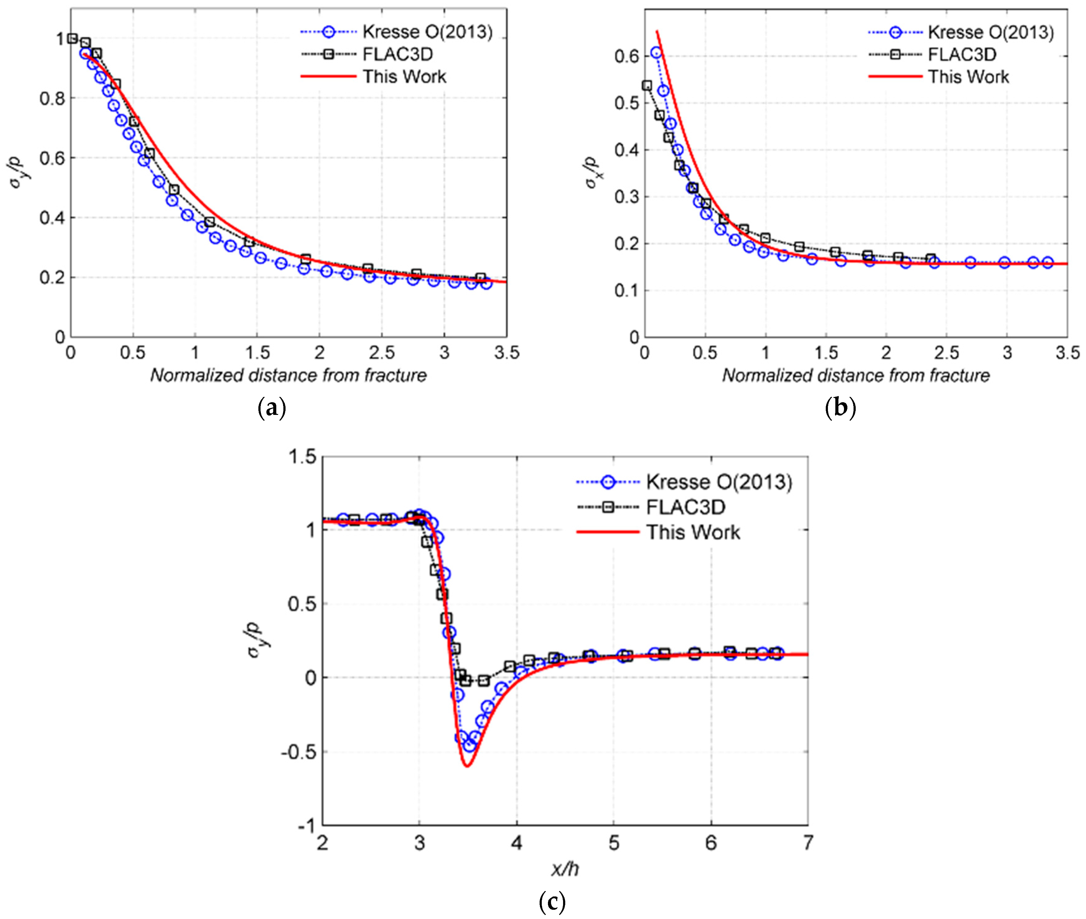
- Kresse, O.; Weng, X.W.; Gu, H.R.; Wu, R.T. Numerical modeling of hydraulic fractures interaction in complex naturally fractured formations. Rock Mech. Rock Eng. 2013, 46, 555–568. [Google Scholar] [CrossRef]
- Weng, X. Modeling of complex hydraulic fractures in naturally fractured formation. J. Unconv. Oil Gas Resour. 2015, 9, 114–135. [Google Scholar] [CrossRef]
- Sesetty, V.; Ghassemi, A. Numerical simulation of sequential and simultaneous hydraulic fracturing. In Proceedings of the ISRM International Conference for Effective and Sustainable Hydraulic Fracturing, Brisbane, Australia, 20–22 May 2013; International Society for Rock Mechanics: Brisbane, Australia, 2013. [Google Scholar]
- Safari, R.; Ghassemi, A. 3D thermo-poroelastic analysis of fracture network deformation and induced micro-seismicity in enhanced geothermal systems. Geothermics 2015, 58, 1–14. [Google Scholar] [CrossRef]
- Verde, A.; Ghassemi, A. Modeling injection/extraction in a fracture network with mechanically interacting fractures using an efficient displacement discontinuity method. Int. J. Rock Mech. Min. Sci. 2015, 77, 278–286. [Google Scholar] [CrossRef]
- Verde, A.; Ghassemi, A. Fast multipole displacement discontinuity method (FM-DDM) for geomechanics reservoir simulations. Int. J. Numer. Anal. Methods Geomech. 2015, 39, 1953–1974. [Google Scholar] [CrossRef]
- Zhang, Z.; Li, X. Numerical study on the formation of shear fracture network. Energies 2016, 9. [Google Scholar] [CrossRef]
- Weng, X.; Kresse, O.; Cohen, C.; Wu, R.; Gu, H. Modeling of hydraulic-fracture-network propagation in a naturally fractured formation. SPE Prod. Oper. 2011, 26, 368–380. [Google Scholar] [CrossRef]
- Zhang, X.; Jeffrey, R. Development of fracture networks through hydraulic fracture growth in naturally fractured reservoirs. In Proceedings of the ISRM International Conference for Effective and Sustainable Hydraulic Fracturing, Brisbane, Australia, 20–22 May 2013; International Society for Rock Mechanics: Brisbane, Australia, 2013. [Google Scholar]
- Olson, J.E. Predicting fracture swarms—The influence of subcritical crackgrowth and the crack-tip process zone on joint spacing in rock. In The Initiation, Propagation, and Arrest of Joints and Other Fractures; Geological Society of London Special Publication: London, UK, 2004; Volume 231, pp. 73–87. [Google Scholar]


| Parameter | Value | Parameter | Value |
|---|---|---|---|
| a | 0.5 m | Layer thickness | Infinite |
| Fluid Net Pressure | 30 MPa | 50 MPa | |
| 20 MPa | Young’s Modulus | Pa | |
| Poisson’s ratio | 0.1 | Friction Coefficient | 0.9 |
| Parameter | Value | Parameter | Value |
|---|---|---|---|
| Injection Rate | Layer thickness | 0.3 m | |
| Fluid Viscosity | 0.1 cP | Friction Coefficient | 0.9 |
| Young’s Modulus | Poisson’s ratio | 0.1 | |
| KIC | 1.0 × 10⁶ Pa·m0.5 |
© 2016 by the authors; licensee MDPI, Basel, Switzerland. This article is an open access article distributed under the terms and conditions of the Creative Commons Attribution (CC-BY) license (http://creativecommons.org/licenses/by/4.0/).
Share and Cite
Zhang, Z.; Li, X. The Shear Mechanisms of Natural Fractures during the Hydraulic Stimulation of Shale Gas Reservoirs. Materials 2016, 9, 713. https://doi.org/10.3390/ma9090713
Zhang Z, Li X. The Shear Mechanisms of Natural Fractures during the Hydraulic Stimulation of Shale Gas Reservoirs. Materials. 2016; 9(9):713. https://doi.org/10.3390/ma9090713
Chicago/Turabian StyleZhang, Zhaobin, and Xiao Li. 2016. "The Shear Mechanisms of Natural Fractures during the Hydraulic Stimulation of Shale Gas Reservoirs" Materials 9, no. 9: 713. https://doi.org/10.3390/ma9090713