
Two Independent Prospectively Planned Blinded Weibull Statistical Analyses of Flexural Strength Data of Zirconia Materials


Abstract
:1. Introduction
1.1. Motivation for a Weibull Analysis
1.2. Motivation for a Prospectively Planned Independent/Parallel Blinded Statistical Analysis
2. Material and Methods
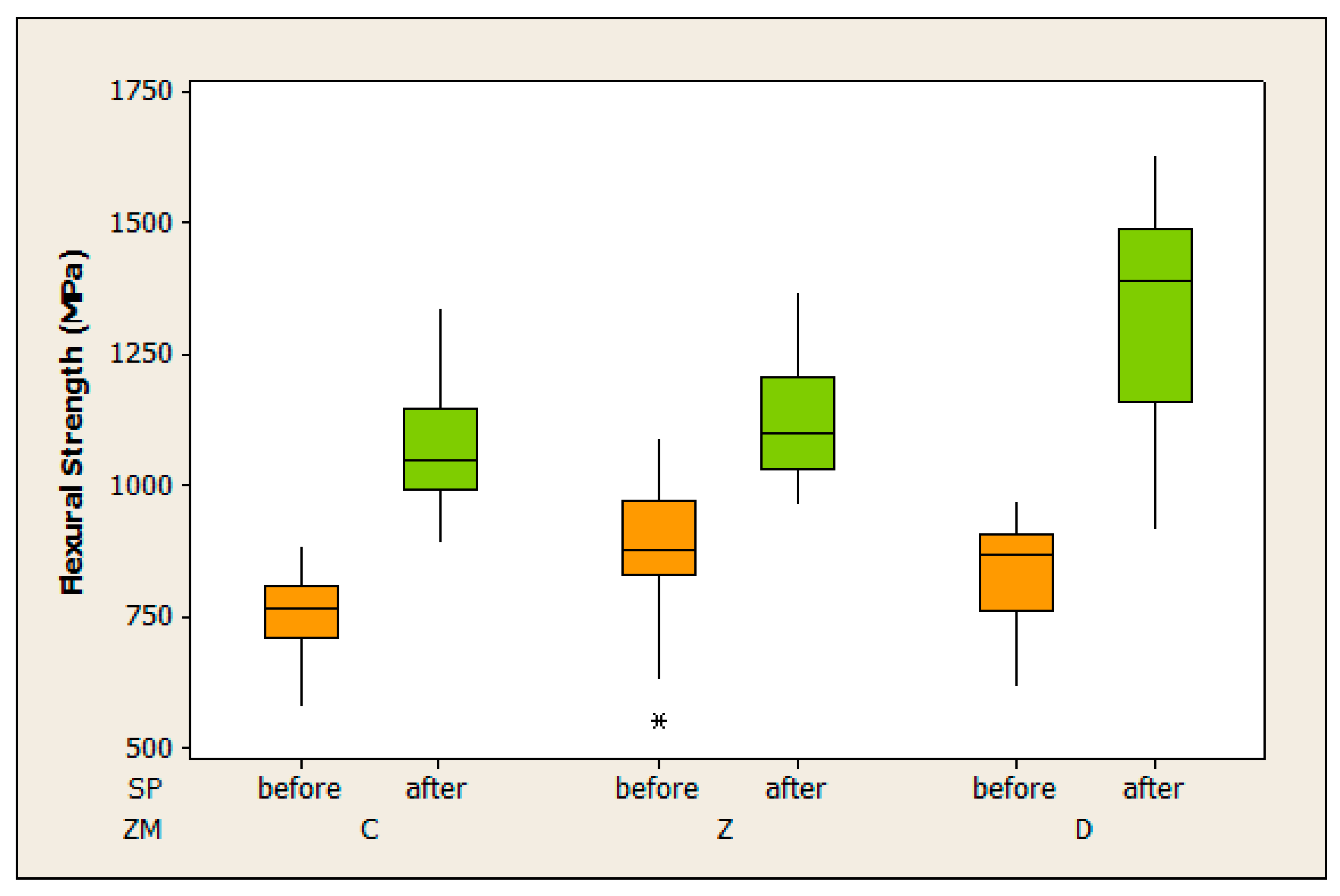
2.1. Experimental Data Description
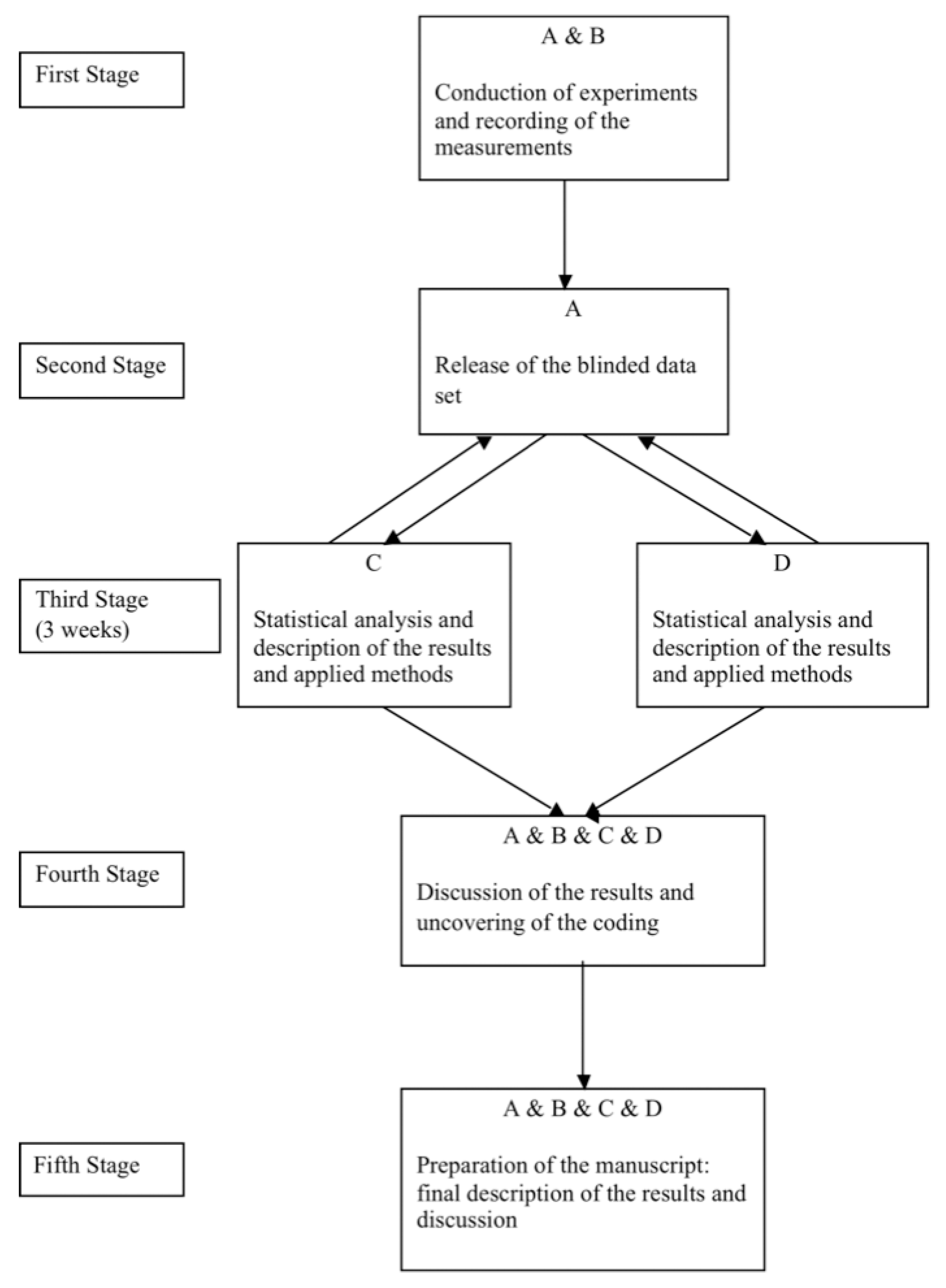
2.2. A prospectively Planned Independent Blinded Statistical Analysis
2.3. Statistical Methods
- ordered p-values: p1 ≤ p2 ≤ ... ≤ pk
- adjusted p-values: piadj = maxj≤i [(k-j + 1) pj]1
- where [x]1 = min(x,1) and i = 1, 2, ..., k
3. Results
4. Discussion
5. Conclusions
- Zirconia specimen preparation method has an impact on characteristic strength (s) and mean of the biaxial flexural strength but in majority of tested groups practically no relevant impact on modulus (m) and standard deviation (sd) of the results.
- All three tested zirconia materials showed different characteristics strengths and mean flexural strength results. Group G6 (D/after) showed higher spread leading to smaller modulus and increased sd estimates.
- The “blinded data set”, “independent statistical analyses” and “parallel manuscript writing” techniques had an influence on the findings for strength data. The impact of “independent statistical analyses” was most pronounced.
- Statistical analysis paths taken by both independently working biostatisticians differed.
- The major difference in the findings was caused by two alternative distributional assumptions (Weibull/Normal) and alternative estimation methods (LS/ML).
Acknowledgments
Author Contributions
Conflicts of Interest
References
- Stawarczyk, B.; Özcan, M.; Hallmann, L.; Ender, A.; Mehl, A.; Hämmerle, C.H.F. The effect of zirconia sintering temperature on flexural strength, grain size, and contrast ratio. Clin. Oral Investig. 2012, 17, 269–274. [Google Scholar] [CrossRef] [PubMed] [Green Version]
- Stawarczyk, B.; Özcan, M.; Trottmann, A.; Hämmerle, C.H.F.; Roos, M. Evaluation of flexural strength of hipped and presintered zirconia using different estimation methods of Weibull statistics. J. Mech. Behav. Biomed. Mater. 2012, 10, 227–234. [Google Scholar] [CrossRef] [PubMed] [Green Version]
- Schatz, C.; Strickstrock, M.; Roos, M.; Edelhoff, D.; Eichberger, M.; Zylla, I.M.; Stawarczyk, B. Influence of specimen preparation and test methods on the flexural strength results of monolithic zirconia materials. Materials 2016. [Google Scholar] [CrossRef]
- McCabe, J.F.; Carrick, T.E. A statistical approach to the mechanical testing of dental materials. Dent. Mater. 1986, 2, 139–142. [Google Scholar] [CrossRef]
- Danzer, R.; Lube, T.; Supancic, P.; Damani, R. Fracture of ceramics. Adv. Eng. Mater. 2008, 10, 275–298. [Google Scholar] [CrossRef]
- Roos, M.; Stawarczyk, B. Evaluation of bond strength of resin cements using different general-purpose statistical software packages for two-parameter Weibull statistics. Dent. Mater. 2012, 28, e76–e88. [Google Scholar] [CrossRef] [PubMed] [Green Version]
- Nohut, S. Influence of sample size on strength distribution of advanced ceramics. Ceram. Int. 2014, 40, 4285–4295. [Google Scholar] [CrossRef]
- Stawarczyk, B.; Özcan, M.; Hämmerle, C.H.F.; Roos, M. The fracture load and failure types of veneered anterior zirconia crowns: An analysis of normal and Weibull distribution of complete and censored data. Dent. Mater. 2012, 28, 478–487. [Google Scholar] [CrossRef] [PubMed] [Green Version]
- Nelson, W. Applied Life Data Analysis; John Wiley & Sons, Inc.: New York, NY, USA, 1982. [Google Scholar]
- Quinn, J.B.; Quinn, G.D. A practical and systematic review of Weibull statistics for reporting strengths of dental materials. Dent. Mater. 2010, 26, 135–147. [Google Scholar] [CrossRef] [PubMed]
- Abernethy, R. The New Weibull Handbook, 5th ed.; Robert, B.A., Ed.; Robert. Abernethy: North Palm Beach, FL, USA, 2009. [Google Scholar]
- Rinne, H. The Weibull Distribution: A Handbook; Chapman & Hall/CRC Press: Giessen, Germany, 2009. [Google Scholar]
- Bütikofer, L.; Stawarczyk, B.; Roos, M. Two regression methods for estimation of a two-parameter Weibull distribution for reliability of dental materials. Dent. Mater. 2015, 31, e33–e50. [Google Scholar] [CrossRef] [PubMed]
- Greenland, S. Bayesian perspectives for epidemiological research: I. Foundations and basic methods. Int. J. Epid. 2006, 35, 765–775. [Google Scholar] [CrossRef] [PubMed]
- Pocock, S.J.; Hughes, M.D.; Lee, R.J. Statistical problems in the reporting of clinical trials. N. Eng. J. Med. 1987, 317, 426–432. [Google Scholar] [CrossRef] [PubMed]
- Polit, D.F. Blinding during the analysis of research data. Int. J. Nursing Stud. 2011, 48, 636–641. [Google Scholar] [CrossRef] [PubMed]
- Gøtzsche, P.C. Blinding during data analysis and writing of manuscripts. Contr. Clin. Trials 1996, 17, 285–293. [Google Scholar] [CrossRef]
- Pocock, S.J. Clinical Trials: A Practical Approach; John Wiley & Sons: New York, NY, USA, 1983. [Google Scholar]
- Doll, R. Controlled trials: The 1948 watershed. Br. Med. J. 1998, 317, 1217–1220. [Google Scholar] [CrossRef]
- Schulz, K.F.; Chalmers, I.; Altman, D.G. The landscape and lexicon of blinding in randomized trials. Ann. Internal. Med. 2002, 136, 254–259. [Google Scholar] [CrossRef]
- Schulz, K.F.; Altman, D.G.; Moher, D. CONSORT 2010 Statement: Updated guidelines for reporting parallel group randomization trials. Ann. Internal. Med. 2010, 152, 726–732. [Google Scholar] [CrossRef] [PubMed]
- Moher, D.; Hopewell, S.; Schulz, K.F.; Montori, V.; Gøtzsche, P.C.; Devereaux, P.J.; Elbourne, D.; Egger, M.; Altman, D. CONSORT 2010 Explanation and Elaboration: Updated guidelines for parallel group randomized trials. J. Clin. Epidemiol. 2010, 340, c869. [Google Scholar] [CrossRef] [PubMed]
- Miller, L.E.; Stewart, M.E. The blind leading the blind: Use and misuse of blinding randomized controlled trials. Contemp. Clin. Trials 2011, 32, 240–243. [Google Scholar] [CrossRef] [PubMed]
- Schulz, K.F.; Grimes, D.A. Blinding in randomised trials: Hiding who got what. Lancet 2002, 359, 696–700. [Google Scholar] [CrossRef]
- Klein, J.R.; Roodman, A. Blind analysis in nuclear and particle physics. Annu. Rev. Nucl. Part. Sci. 2005, 55, 141–163. [Google Scholar] [CrossRef]
- Dentistry-Ceramic Materials; ISO. 6872:2008; International Organization for Standardization: Geneva, Switzerland, 2008.
- R Foundation for Statistical Computing. A Language and Environment for Statistical Computing; R Foundation for Statistical Computing: Vienna, Austria, 2010; Available online: http://www.R-project.org (accessed on 22 June 2016).
- Holm, S. A simple sequentially rejective multiple test procedure. Scand. J. Stat. 1979, 6, 65–70. [Google Scholar]
- Ryan, B.F.; Joiner, B.L. Minitab 14 Statistical Software; Minitab, Inc.: State College, PA, USA; pp. 1972–2005.
- Johnson, V.E. Revised standards for statistical evidence. Proc. Natl. Acad. Sci. USA 2013, 48, 19313–19317. [Google Scholar] [CrossRef] [PubMed]
- Pocock, S.J. Clinical trials with multiple outcomes: A statistical perspective on their design, analysis and interpretation. Control. Clin. Trials 1997, 18, 530–545. [Google Scholar] [CrossRef]
- Watthanacheewakul, L. Analysis of Variance with Weibull Data. In Proceedings of the International MultiConference of Engineers and Computer Scientists, Hong Kong, China, 16–18 March 2011; Volume 3, pp. 2051–2056.
- Hannigan, A.; Lynch, C.D. Statistical methodology in oral and dental research: Pitfalls and recommendations. J. Dent. 2013, 41, 385–392. [Google Scholar] [CrossRef] [PubMed]


| Study Phase | Uncertainty Source |
|---|---|
| Data generation (a) | Specimens/Subjects Investigators Data collectors and managers Precision of measuring devices Outcome assessors |
| Statistical data analysis (b) | Sample size Data analyst Descriptive statistics Assumption on the sampling distribution (model uncertainty) Outliers (data uncertainty) Choice of the statistical approach (frequentist or Bayesian) If Bayesian, then prior elicitation (prior uncertainty) Transformation of variables Parametric or non-parametric analysis Tests/Confidence intervals Choice of the estimation technique within the approach chosen Interpretation of the results Missing data handling Subgroup analysis Covariates selection |
| Writing of the manuscript (c) | Choice of the findings to report on Choice of the graphs to be shown Manuscript writer |
| Tested Groups | ZM | SP | n | Min | q1 | Mean | Median | q2 | Max | sd |
|---|---|---|---|---|---|---|---|---|---|---|
| G1 | C | before | 40 | 575 | 719 | 757 | 765 | 804 | 884 | 79 |
| G2 | C | after | 40 | 890 | 997 | 1077 | 1050 | 1143 | 1340 | 113 |
| G3 | Z | before | 40 | 551 | 842 | 891 | 878 | 966 | 1090 | 115 |
| G4 | Z | after | 40 | 962 | 1030 | 1126 | 1100 | 1203 | 1370 | 114 |
| G5 | D | before | 40 | 615 | 764 | 835 | 869 | 908 | 969 | 102 |
| G6 | D | after | 40 | 915 | 1180 | 1322 | 1390 | 1490 | 1630 | 214 |
| Tested Groups | ZM | SP | Method | m | 95% CI (m) | s | 95% CI (s) |
|---|---|---|---|---|---|---|---|
| G1 | C | before | ML YonX/hazen | 11.4 11.4 | [8.9, 14.6] [8.2, 15.9] | 791 791 | [768, 814] [768, 814] |
| G2 | C | after | ML YonX/hazen | 9.6 11.4 | [7.6, 12.0] [8.2, 15.9] | 1129 1126 | [1090, 1168] [1093, 1159] |
| G3 | Z | before | ML YonX/hazen | 9.4 8.9 | [7.3, 11.9] [6.4, 12.4] | 939 942 | [906, 972] [907, 977] |
| G4 | Z | after | ML YonX/hazen | 10.3 11.8 | [8.1, 13.0] [8.5, 16.3] | 1178 1176 | [1141, 1217] [1143, 1210] |
| G5 | D | before | ML YonX/hazen | 10.9 9.5 | [8.3, 14.1] [6.8, 13.2] | 877 880 | [851, 904] [849, 911] |
| G6 | D | after | ML YonX/hazen | 7.9 7.0 | [6.1, 10.3] [5.0, 9.7] | 1409 1414 | [1352, 1468] [1348, 1484] |
| Comparison | Condition | Test Statistic | p-Values | |||
|---|---|---|---|---|---|---|
| m | s | m | s | |||
| (a) | before-after (G1-G2) | C | 0.014 | −334.9 | 0.9830 | <0.0001 |
| before-after (G3-G4) | Z | −2.831 | −234.4 | 0.0370 | NA | |
| before-after (G5-G6) | D | 2.494 | −534.7 | <0.0001 | NA | |
| (b) | C-Z-D (G1-G3-G5) | before | 1.664 | 100.4 | 0.2010 | <0.0001 |
| C-Z-D (G2-G4-G6) | after | 3.186 | 192.4 | <0.0001 | NA | |
| (c) | C-Z (G1-G3) | before | 2.496 | −150.6 | NA | <0.0001 |
| C-D (G1-G5) | before | 1.948 | −88.8 | NA | <0.0001 | |
| Z-D (G3-G5) | before | −0.547 | 61.8 | NA | 0.0080 | |
| C-Z (G2-G4) | after | −0.350 | −50.2 | 0.8210 | 0.0840 | |
| C-D (G2-G6) | after | 4.428 | −288.7 | <0.0001 | NA | |
| Z-D (G4-G6) | after | 4.778 | −238.5 | <0.0001 | NA | |
| Step | Decision/Action |
|---|---|
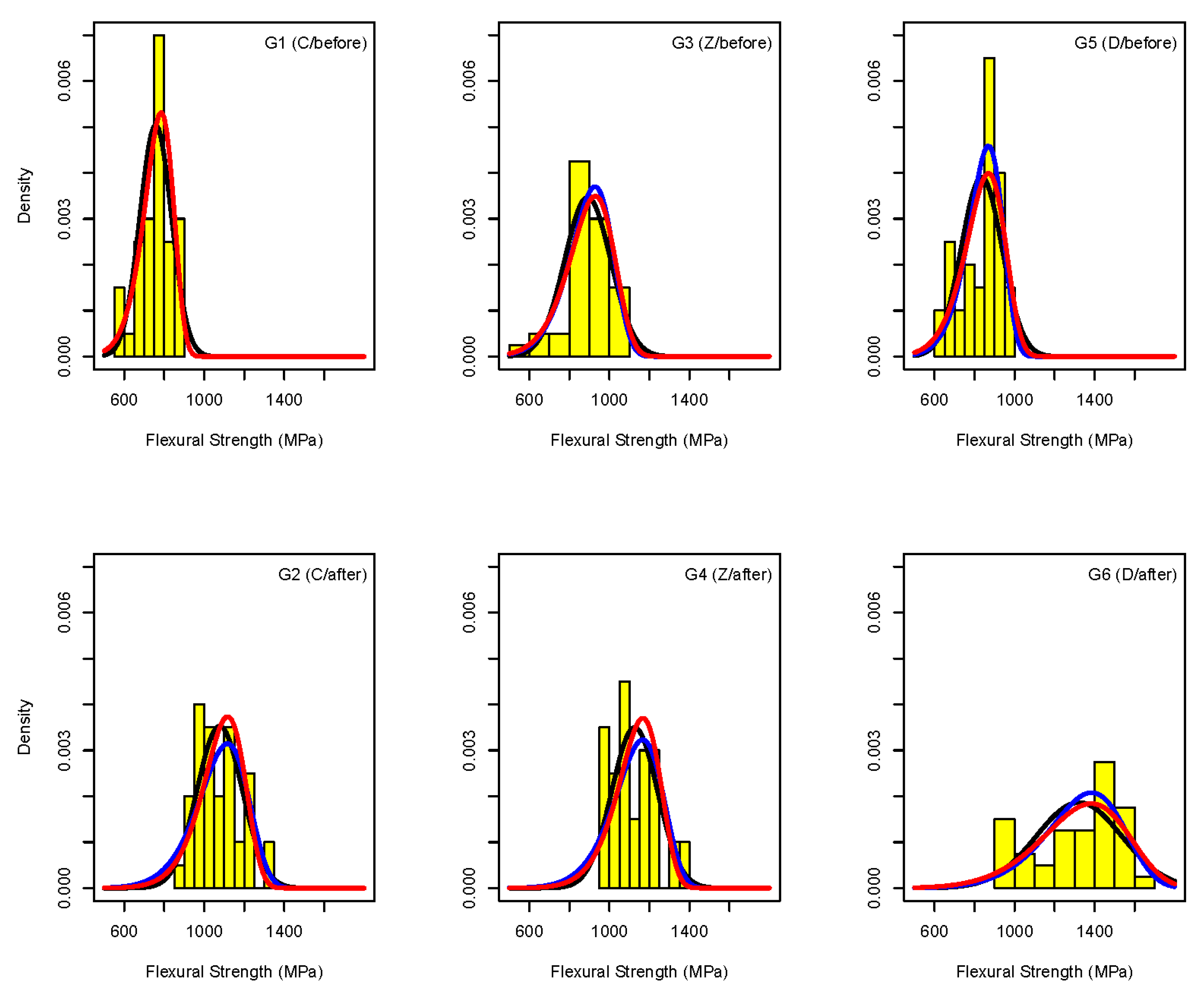
| Step 1 | Data visualization in each tested group (see Figure 2 and Figure 4): Check data visually by histograms, scatterplots and/or boxplots. Are there any outlying observations? If yes, check if they are possibly typing errors and correct them. Are histograms approximately symmetric in each tested group? If no, you may try to transform the measurements. |
| Step 2 | Distributional assumption for measurements (see Section 1.1): Do you think that each measurement consists of a possibly large number of independent random fluctuations? If yes, go for a Normality assumption directly (for approximately symmetrical histograms) or after a (logarithmic) transformation of measurements. Do you believe in the “weakest link” process generating your data? If yes, go for a Weibull assumption. If both assumptions seem to be reasonable use both Normal and Weibull distributional assumptions for your working hypothesis. |
| Step 3 | Descriptive statistics: Estimation of parameters in each tested group: Under Normality assumption: compute mean and standard deviation (sd). Under Weibull assumption: compute the characteristic strength (s) and modulus (m). See the open source Excel-calculator (Appendix C in [13]). Remember: (s “=” mean) and (m “=” 1/sd) (see Section 1.1) |
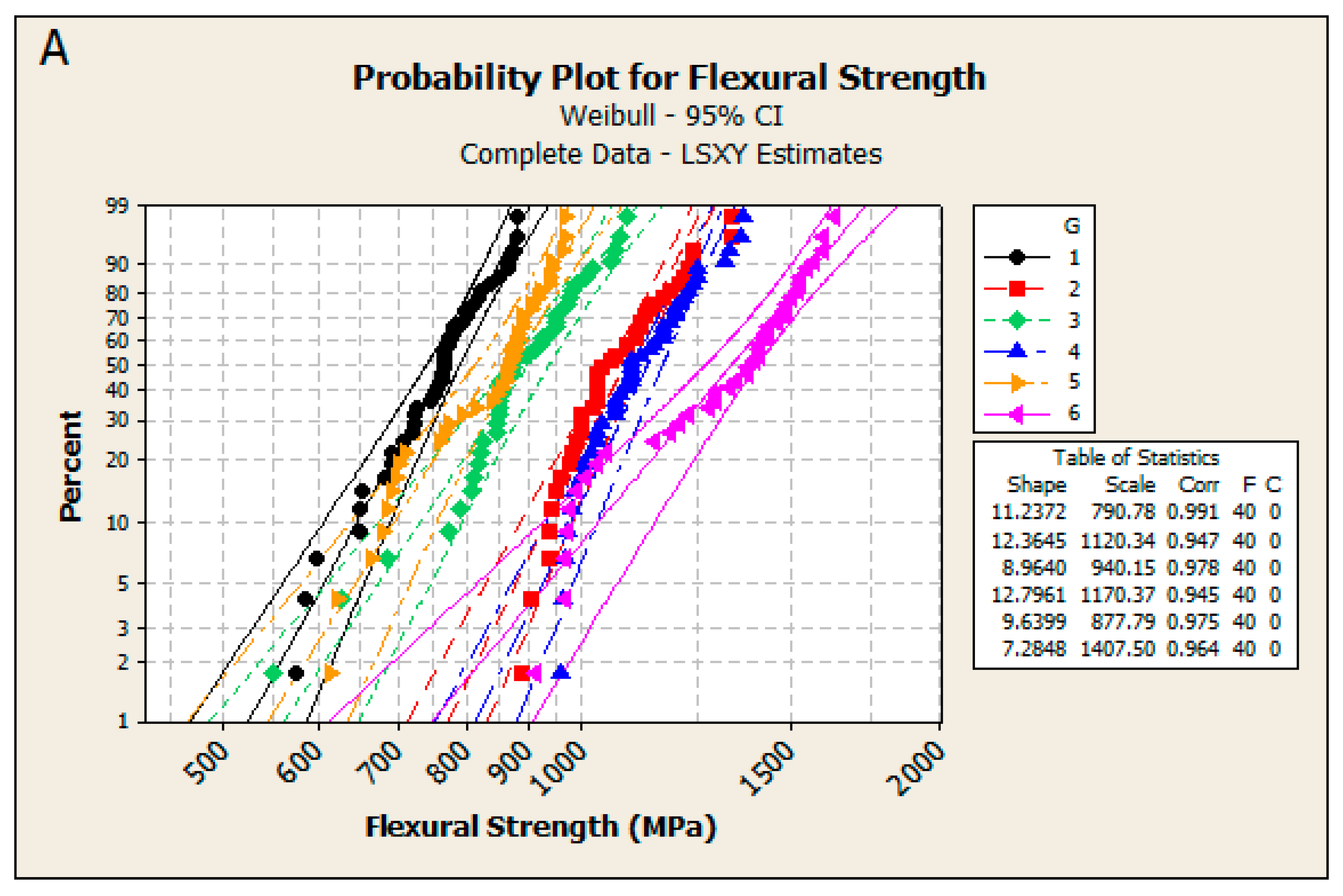
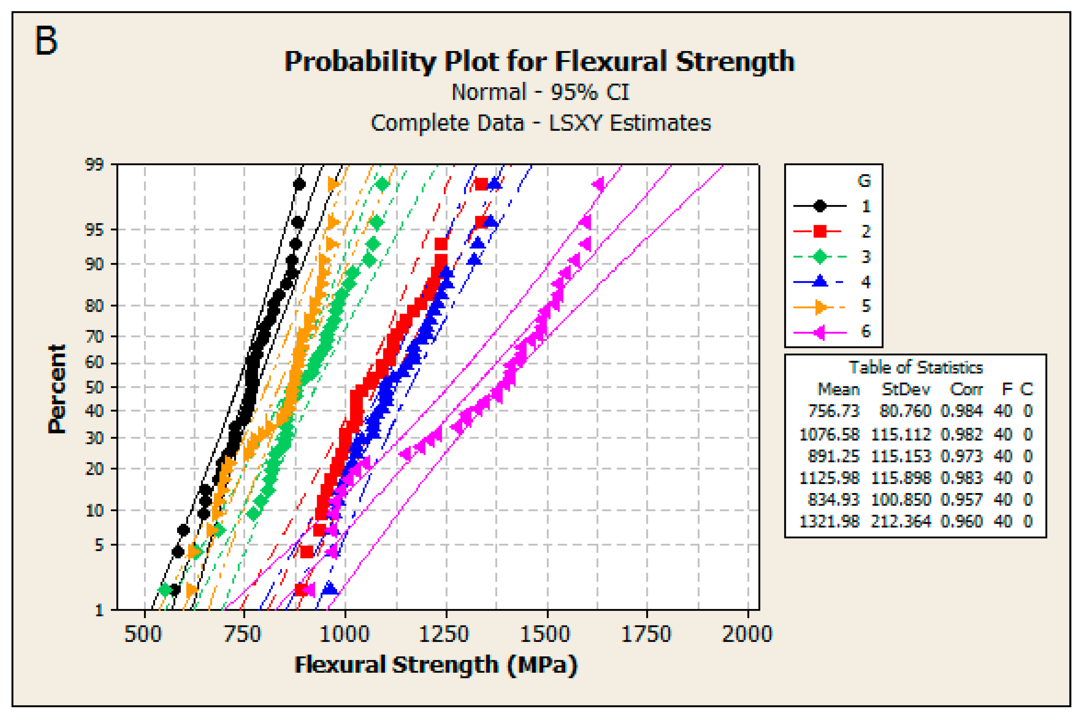
| Step 4 | Check the goodness-of-fit in each tested group: Compute the goodness-of-fit estimates. Generate probability plots (see Figure 3) and check if they are linear. In case of approximate linearity the assumed distribution fits the data well. In case of clear non-linearity interpret the results with caution. |
| Step 5 | Estimation of 95%CI for parameters in each tested group: Under Normality assumption: 95% CI (mean) and 95% CI (sd). Under Weibull assumption: 95% CI (s) and 95% CI (m). See the open source Excel-calculator (Appendix C in [13]). |
| Step 6 | Are there any differences between tested groups? Normal mean: Apply an Analysis of Variance (ANOVA). Normal sd: Apply a Levene-Test. Weibull s and m: Apply the Bartlett’s modified likelihood ratio tests. |
| Step 7 | Check the results: Critically check if the results obtained in Step 6 agree with the graphs generated in Step 1. If you applied both the Normal and the Weibull assumptions critically check if the results obtained in Step 6 are comparable. Remember: (s “=” mean) and (m “=” 1/sd) (See Section 1.1). |
© 2016 by the authors; licensee MDPI, Basel, Switzerland. This article is an open access article distributed under the terms and conditions of the Creative Commons Attribution (CC-BY) license (http://creativecommons.org/licenses/by/4.0/).
Share and Cite
Roos, M.; Schatz, C.; Stawarczyk, B. Two Independent Prospectively Planned Blinded Weibull Statistical Analyses of Flexural Strength Data of Zirconia Materials. Materials 2016, 9, 512. https://doi.org/10.3390/ma9070512
Roos M, Schatz C, Stawarczyk B. Two Independent Prospectively Planned Blinded Weibull Statistical Analyses of Flexural Strength Data of Zirconia Materials. Materials. 2016; 9(7):512. https://doi.org/10.3390/ma9070512
Chicago/Turabian StyleRoos, Malgorzata, Christine Schatz, and Bogna Stawarczyk. 2016. "Two Independent Prospectively Planned Blinded Weibull Statistical Analyses of Flexural Strength Data of Zirconia Materials" Materials 9, no. 7: 512. https://doi.org/10.3390/ma9070512