
Characterization of Thermo-Physical Properties of EVA/ATH: Application to Gasification Experiments and Pyrolysis Modeling

 ,
, 
Abstract
:1. Introduction
2. Experimental Section
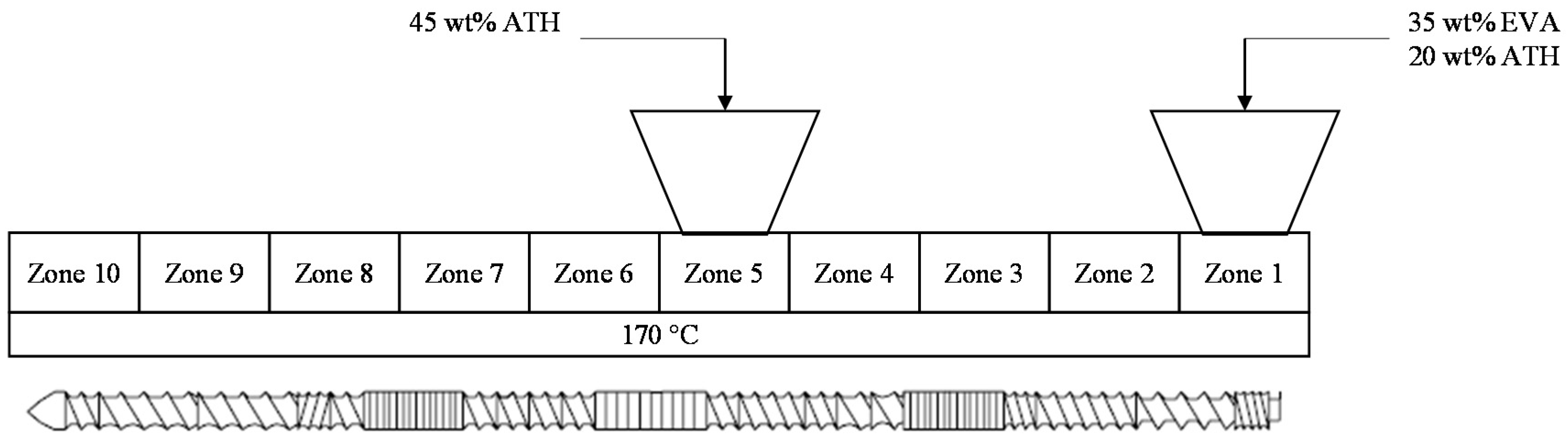
2.1. Material and Sample Preparation
2.2. Thermal Conductivity
2.3. Thermo-Gravimetric Analysis and Kinetic Analysis
2.4. Differential Scanning Calorimetry
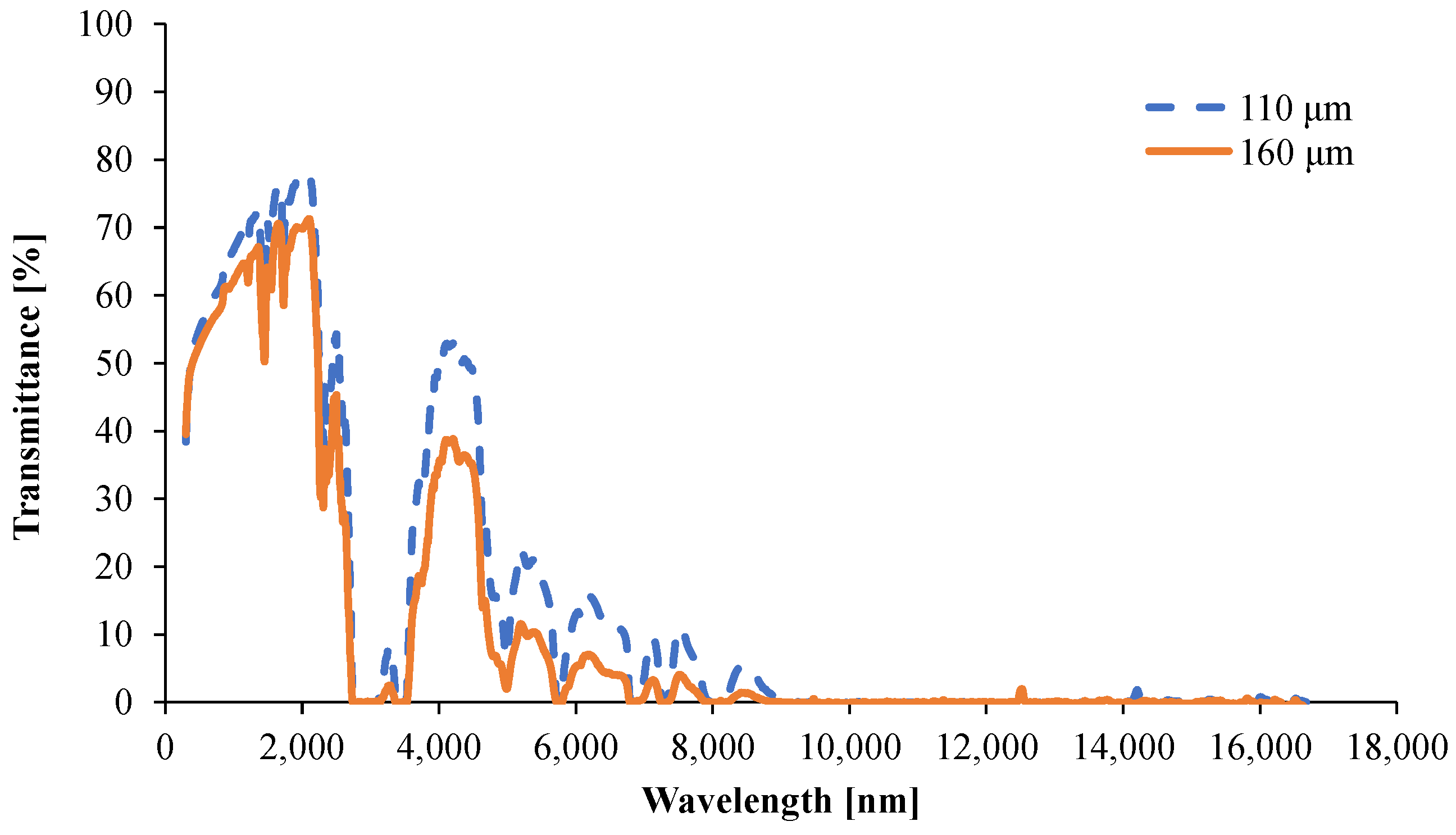
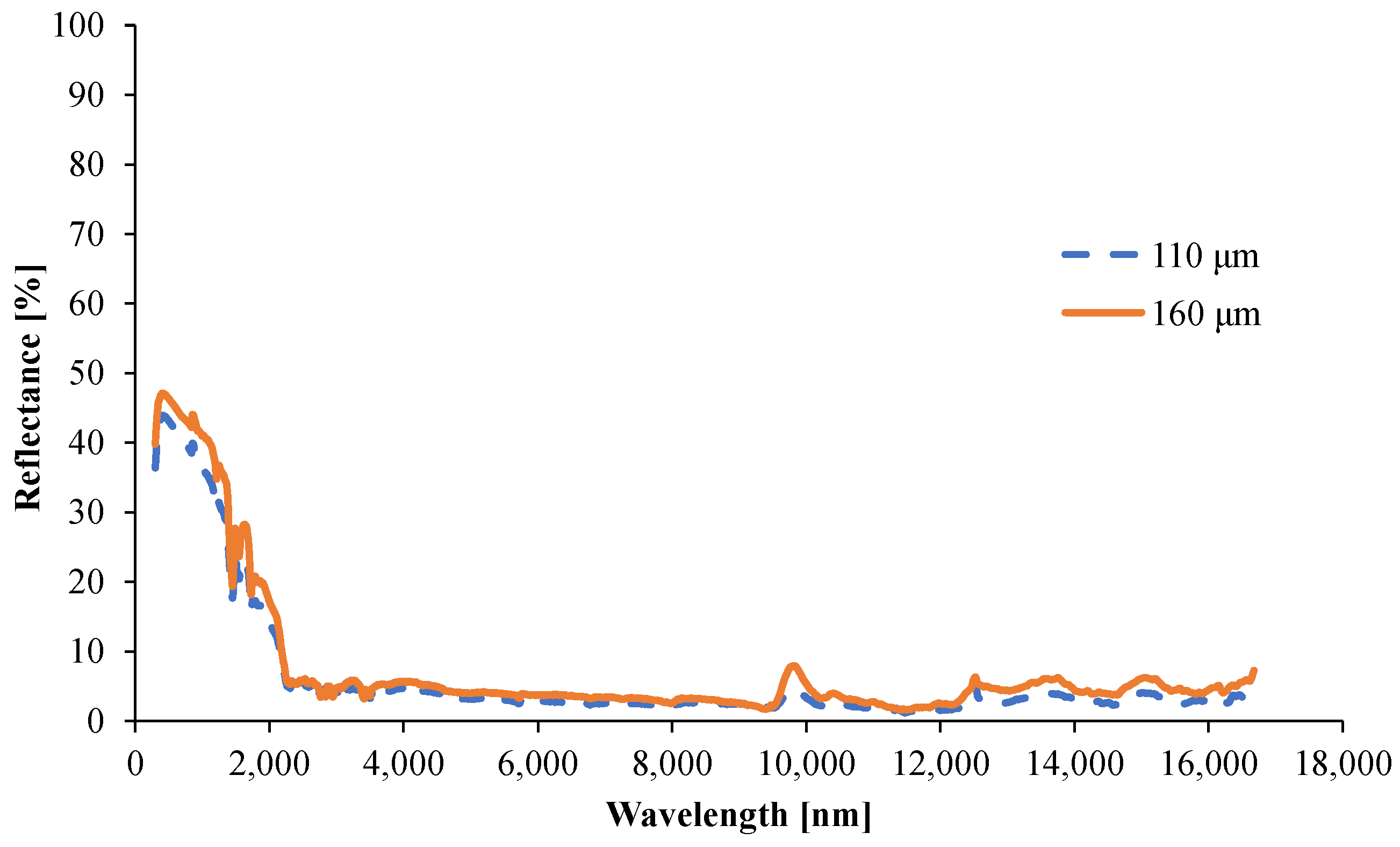
2.5. Optical Measurements
- Tsample,λ is the spectrally resolved transmittance through the entire specimen (measured);
- Tsurface,λ is the spectrally resolved transmittance through one surface of the specimen (not measured);
- Rsurface,λ is the spectrally resolved reflectance from one surface of the specimen (not measured);
- d is the thickness of the sample.
- Rsample,λ is the spectrally resolved reflectance from the entire specimen (measured);
- Rsurface,λ is the spectrally resolved reflectance from one surface of the specimen (not measured).
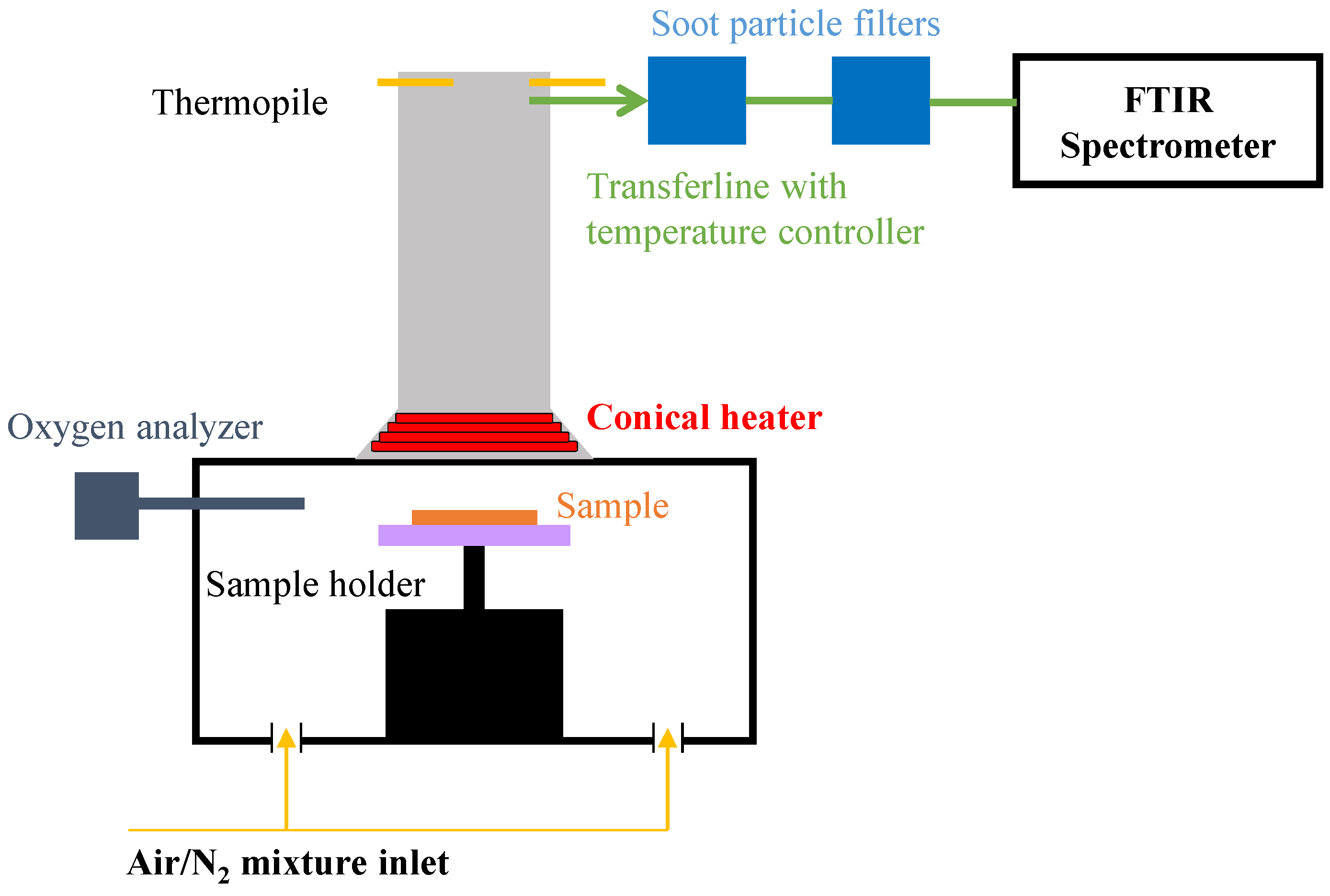
2.6. Gasification Experiments
2.7. Pyrolysis Model Development
3. Results and Discussion
3.1. Determination of Input Data
- -
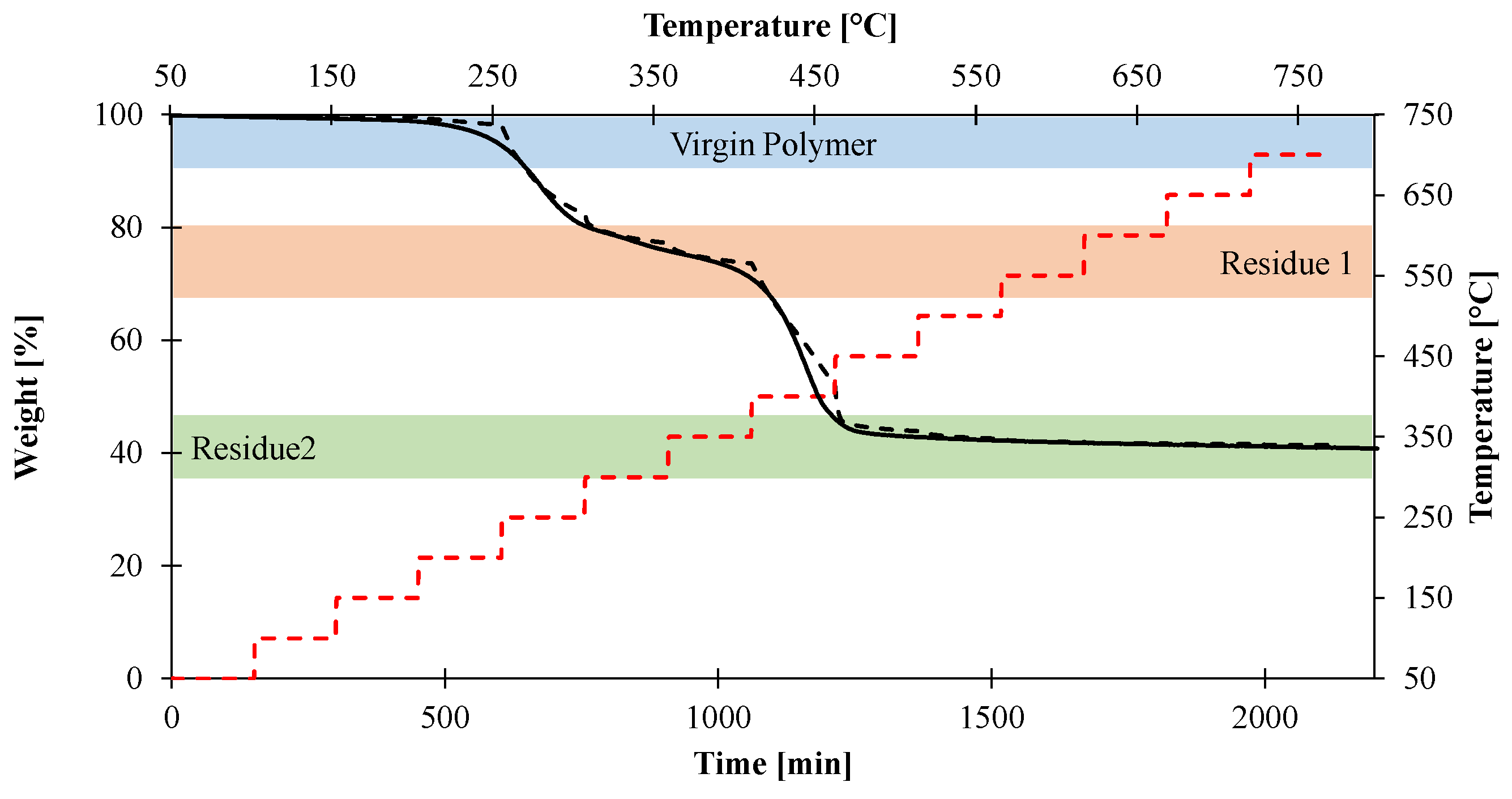
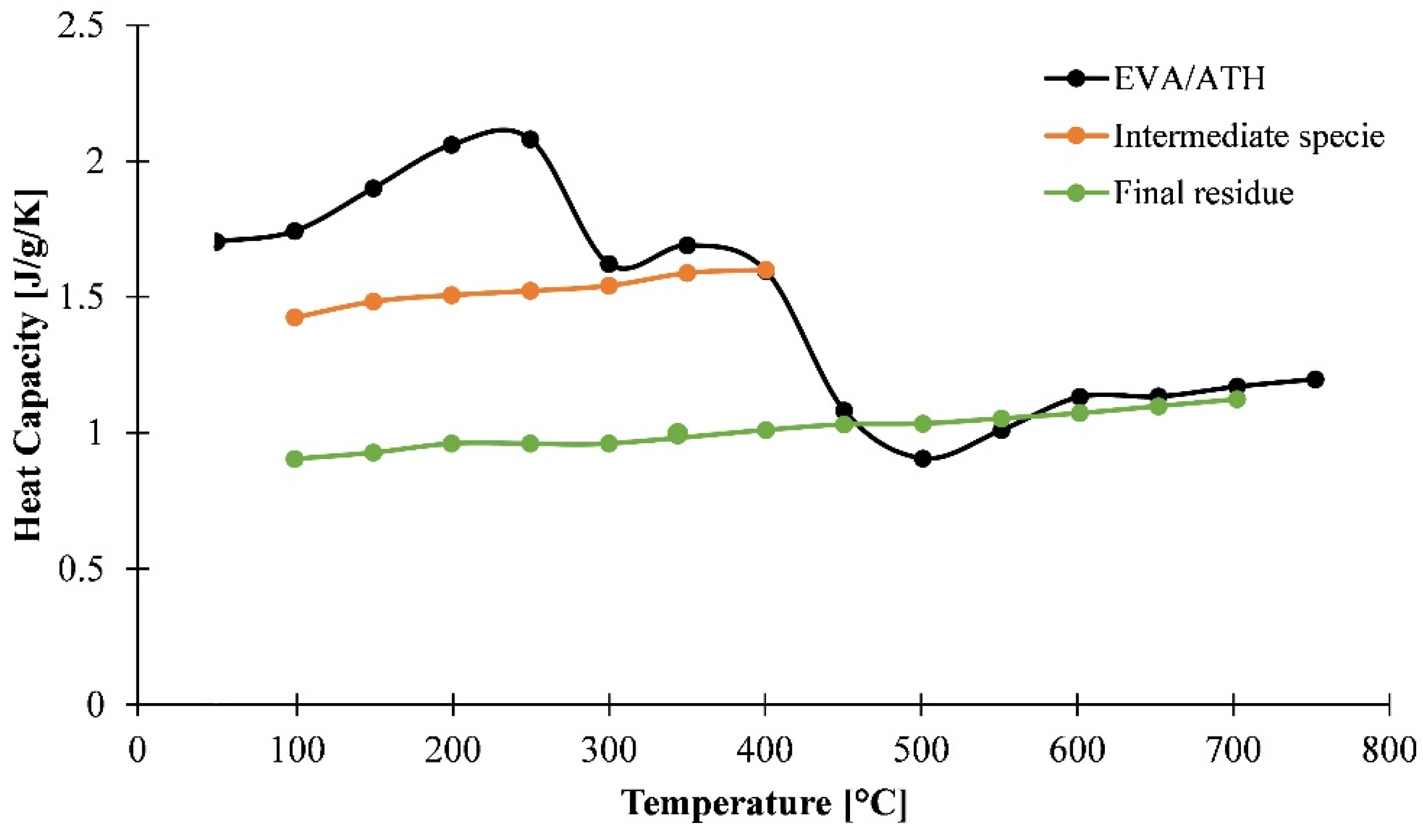
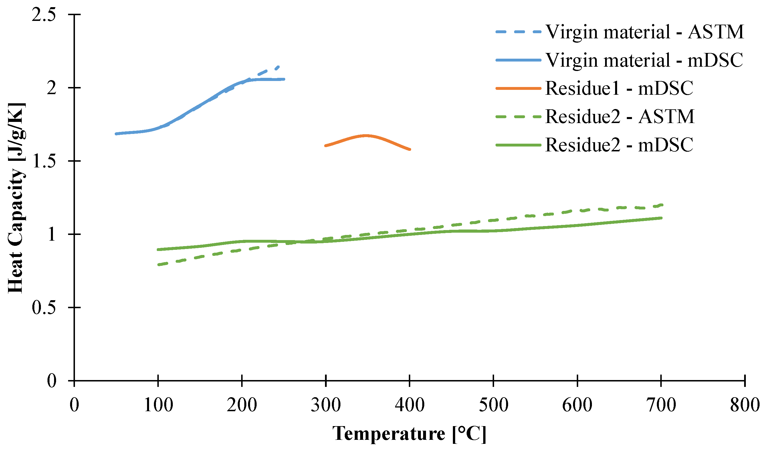
- Virgin material refers to the initial formulation of EVA/ATH.
- -
- -
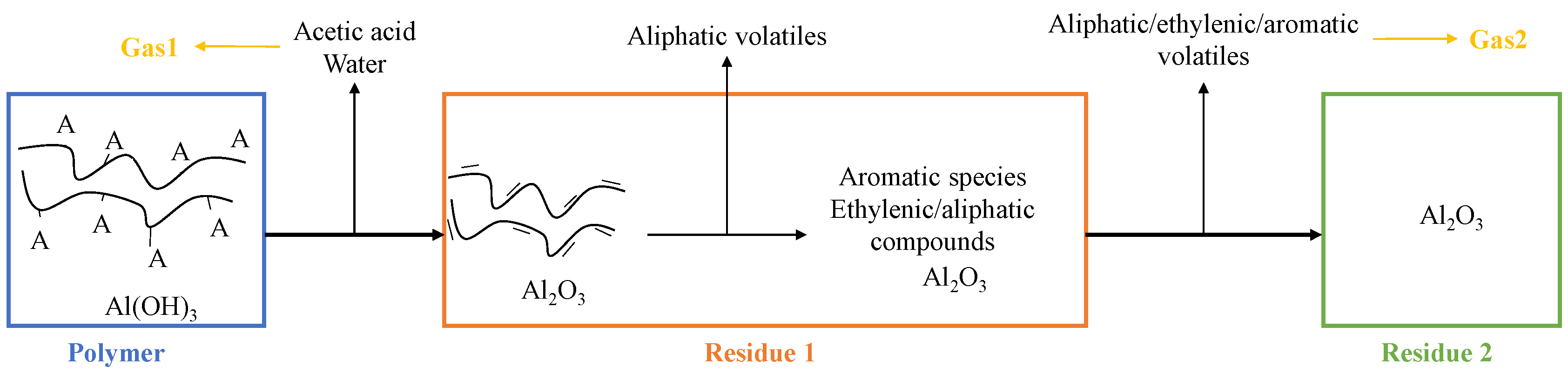
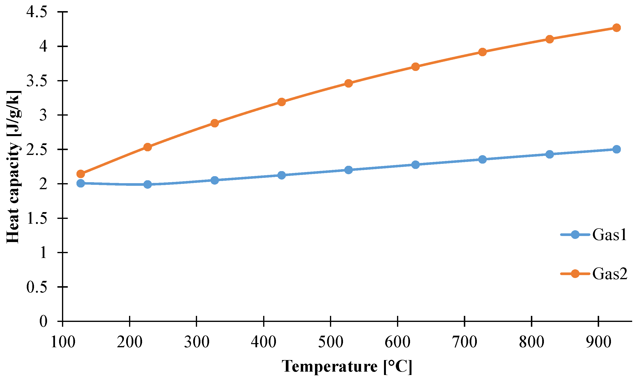
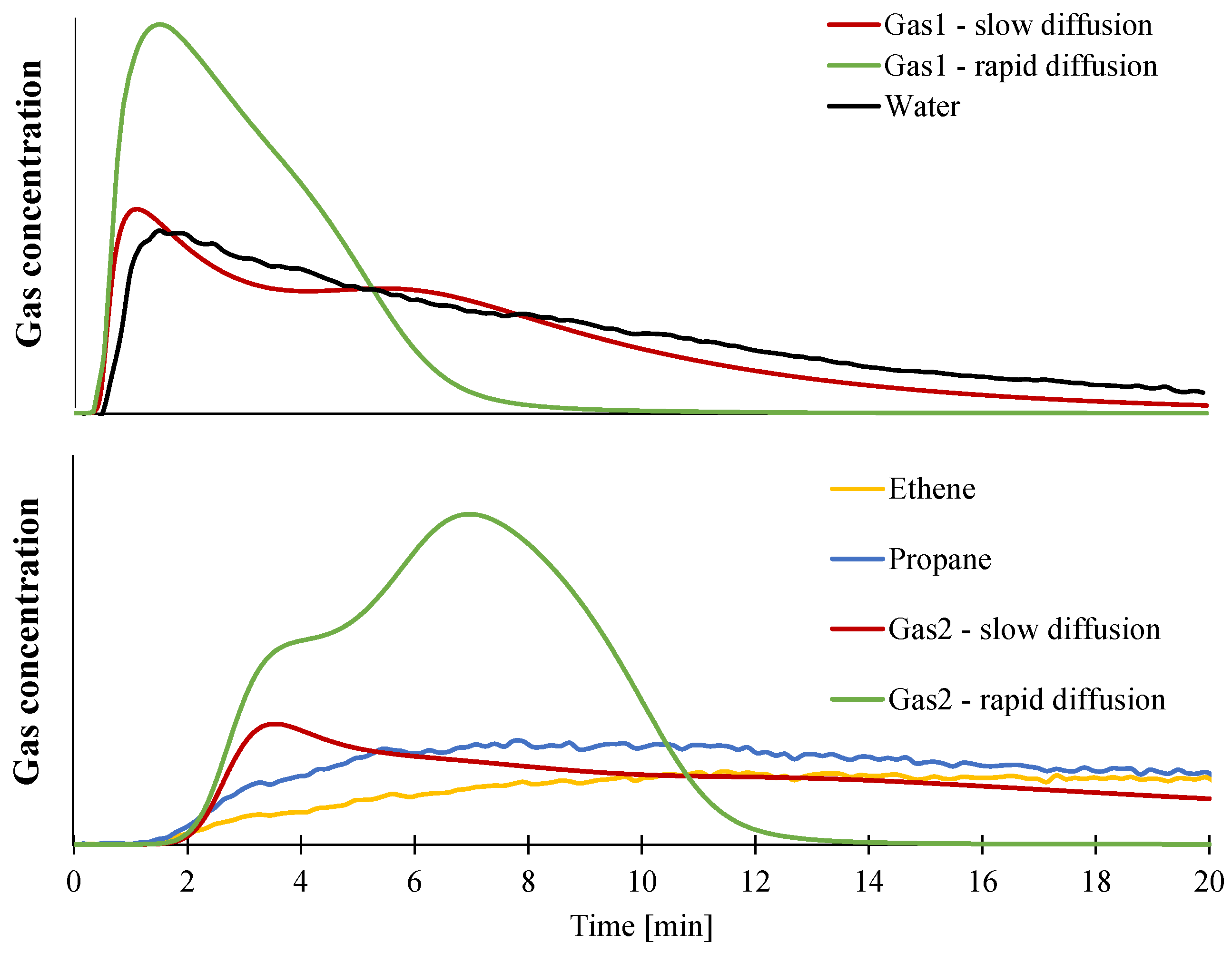
- Gas1 refers to the water released during the decomposition of ATH into alumina, and acetic acid from the deacetylation of the EVA.
- -
- Residue2 refers to the alumina residue. EVA is assumed to be completely degraded.
- -
- Gas2 is a mixture of hydrocarbon gases evolved during the decomposition of the EVA.
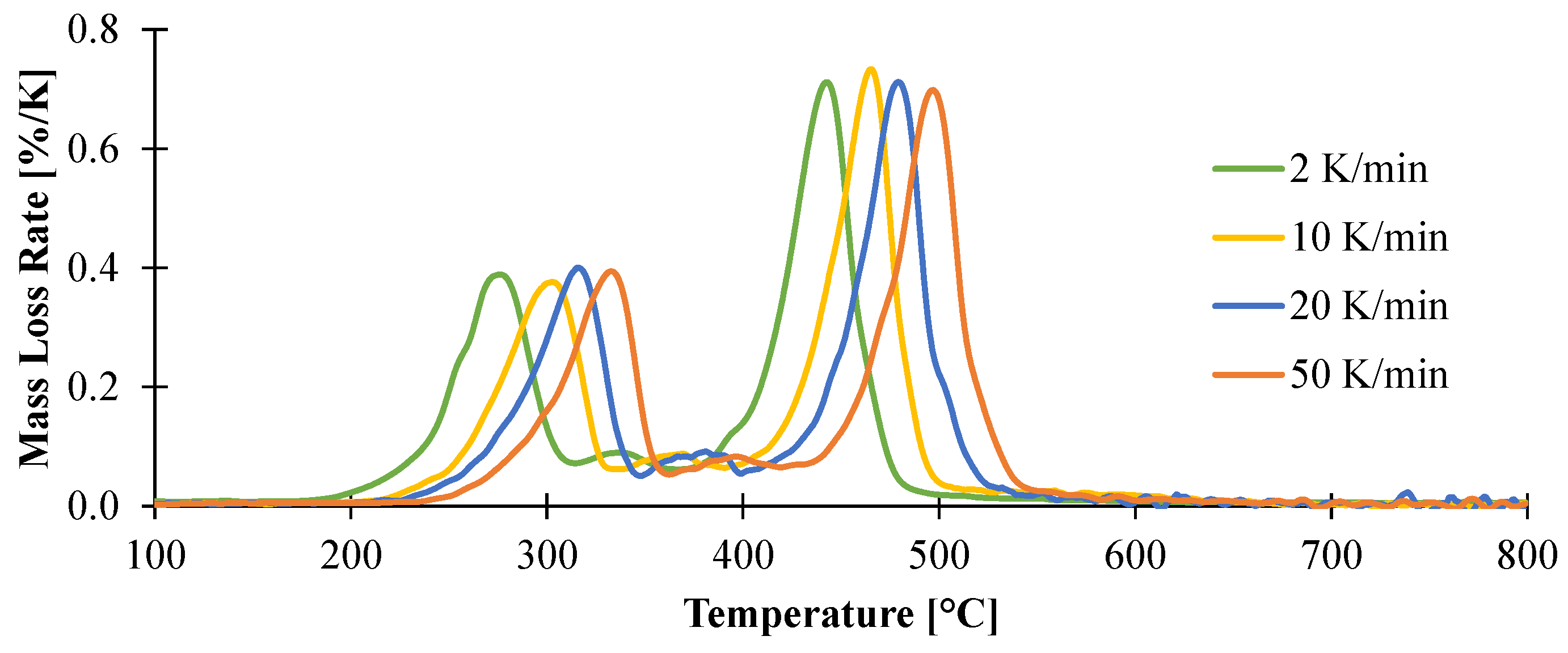
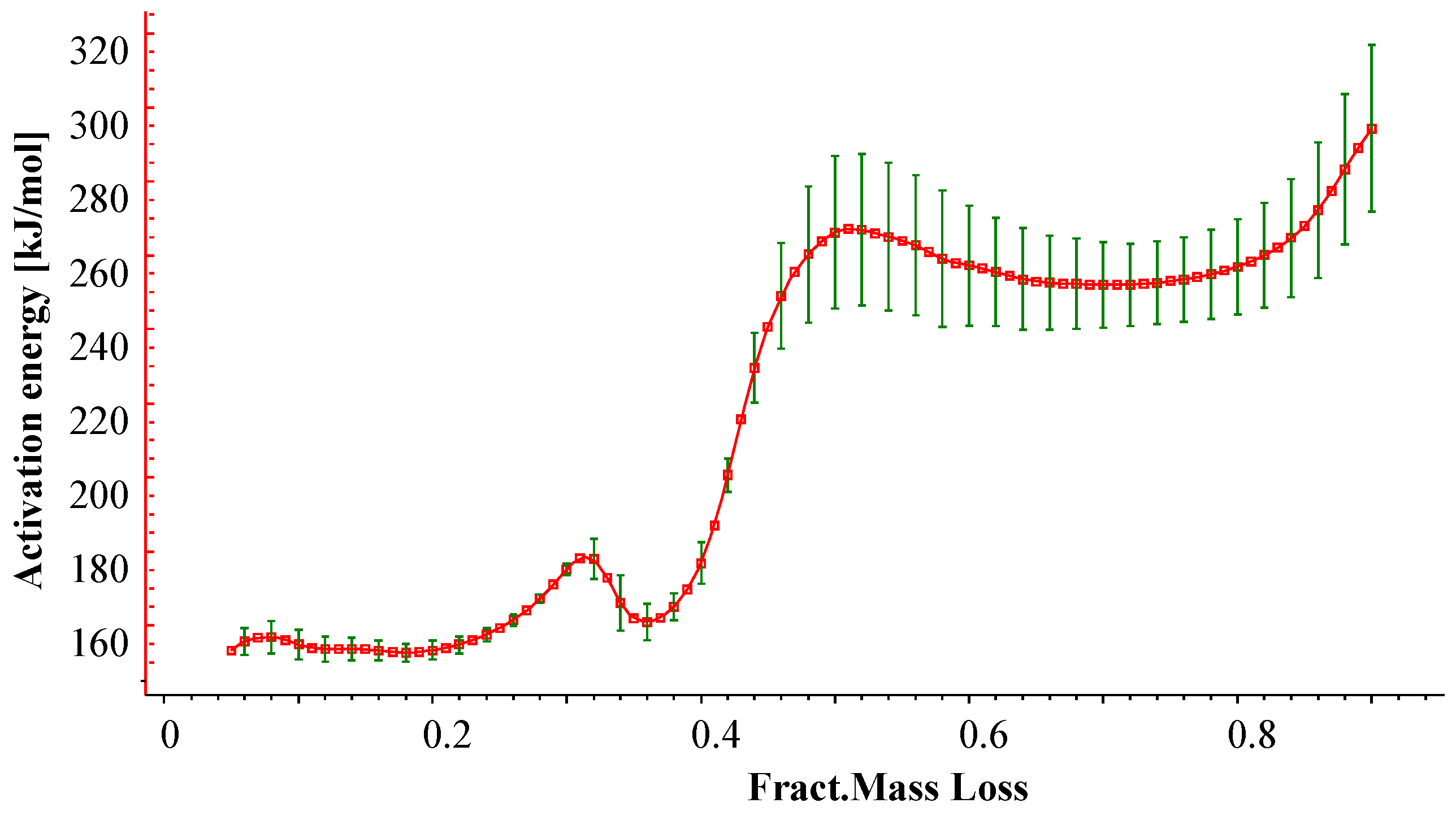
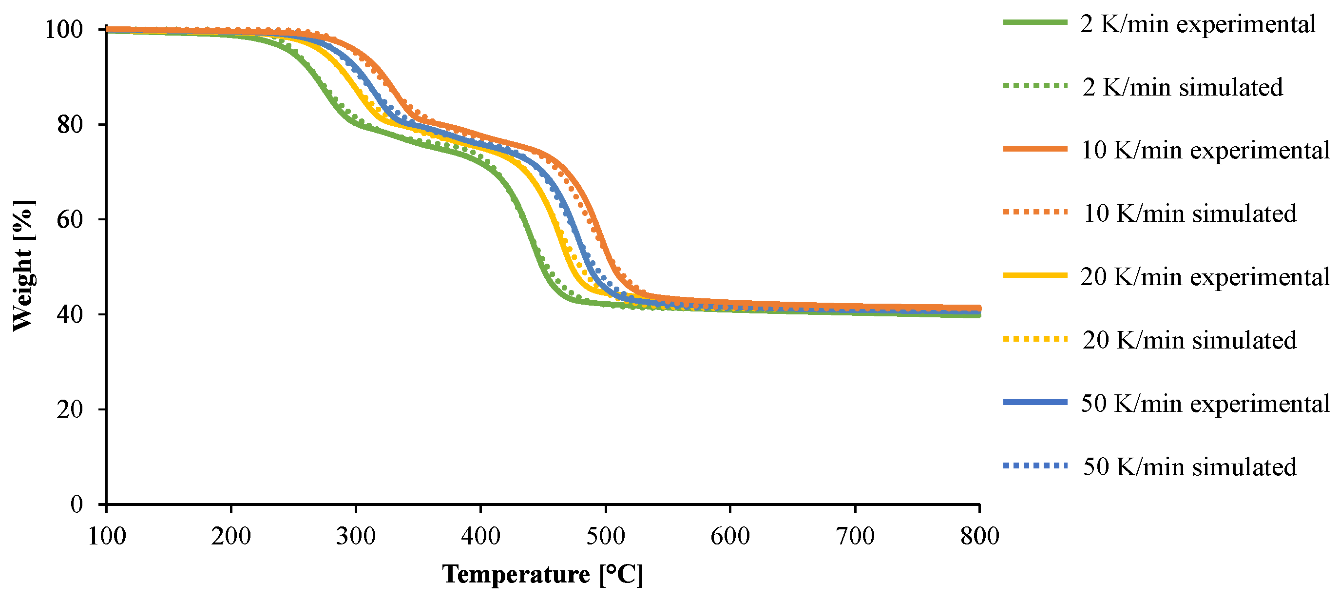
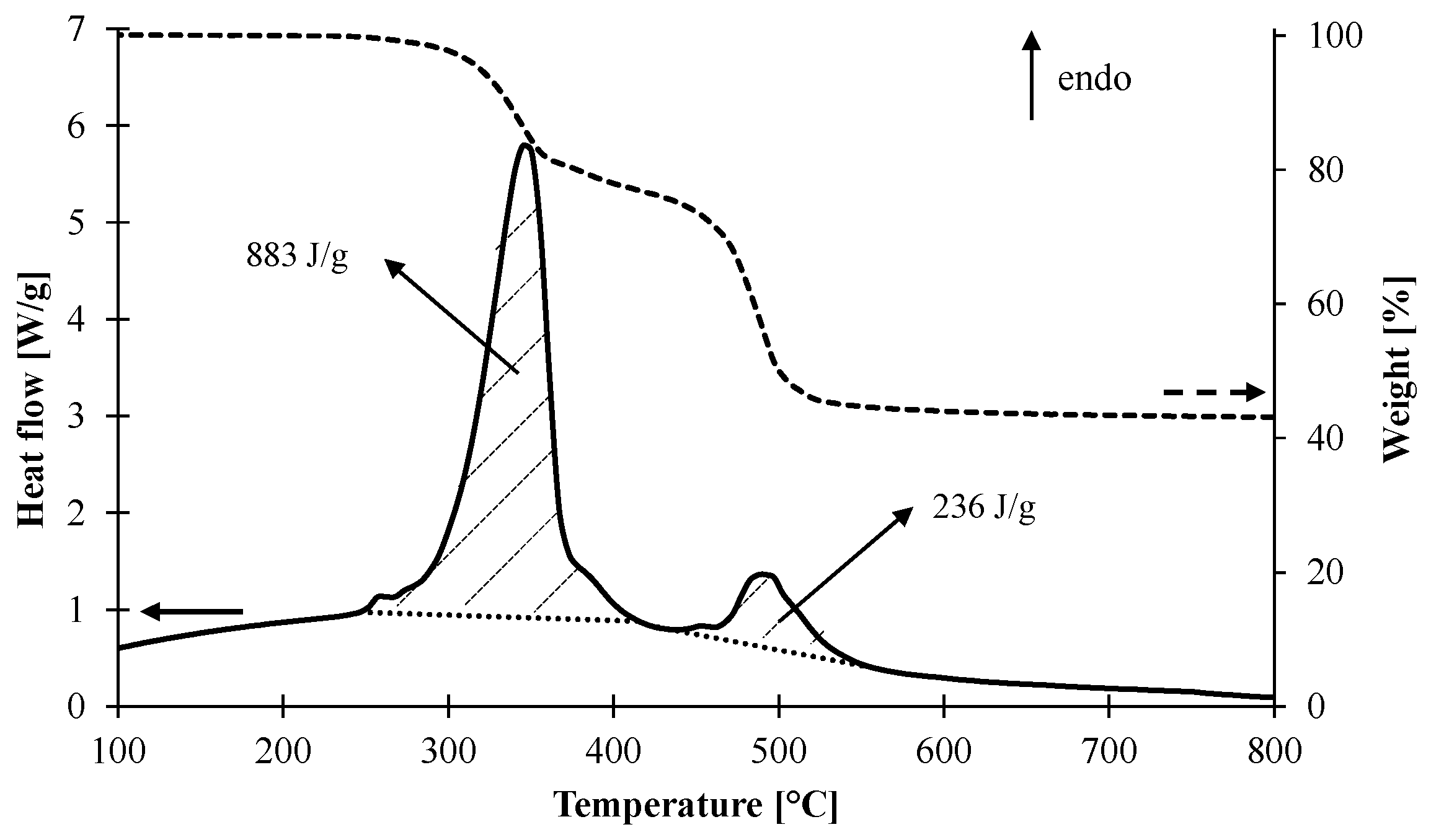
3.1.1. Kinetic Analysis and Determination of the Enthalpies of Reaction


| Reaction | Ar (1/s) | Er (kJ/mol) | Reaction Order | Hr (J/g) |
|---|---|---|---|---|
| 1 | 8.71 × 10¹² | 162 | 3 | 883 |
| 2 | 1.23 × 10¹⁷ | 268 | 2 | 236 |

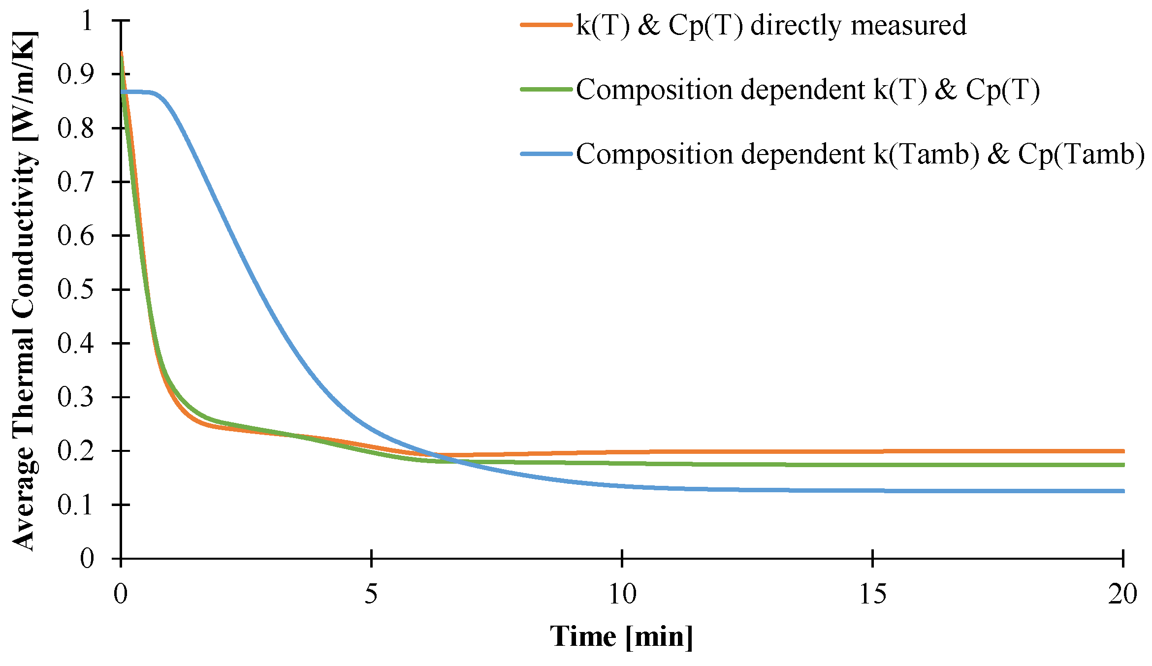
3.1.2. Determination of Thermal Conductivity of the Material as a Function of the Temperature
| Thermal Conductivity (W/m/K) | Temperature Range (°C) |
|---|---|
| 1.17–3.21 × 10⁻³ T | Ambient–250 |
| 0.28 | 250–400 |
| 0.18 | 400–700 |
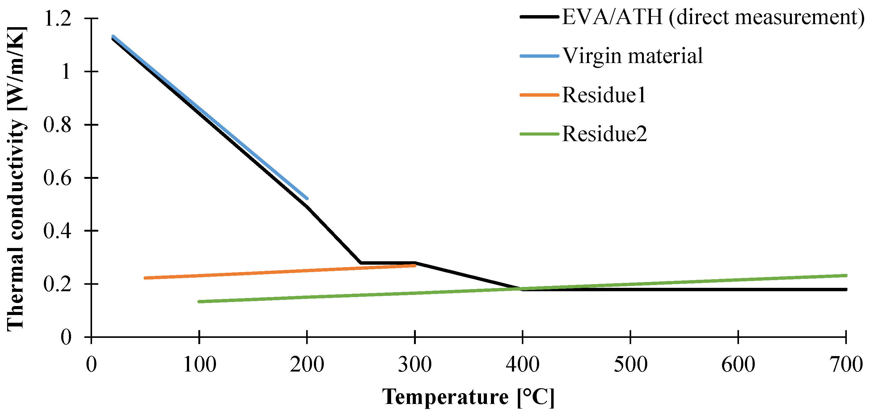

| Thermal Conductivity (W/m/K) | Specie | Temperature Range |
|---|---|---|
| 1.20 – 3.39 × 10⁻³ T | Virgin EVA/ATH | <250 °C |
| 0.21 + 1.89 × 10⁻⁴ T | Residue1 | <350 °C |
| 0.11 + 1.63 × 10⁻⁴ T | Residue2 | >400 °C |
3.1.3. Determination of Heat Capacity of the Material as a Function of the Temperature


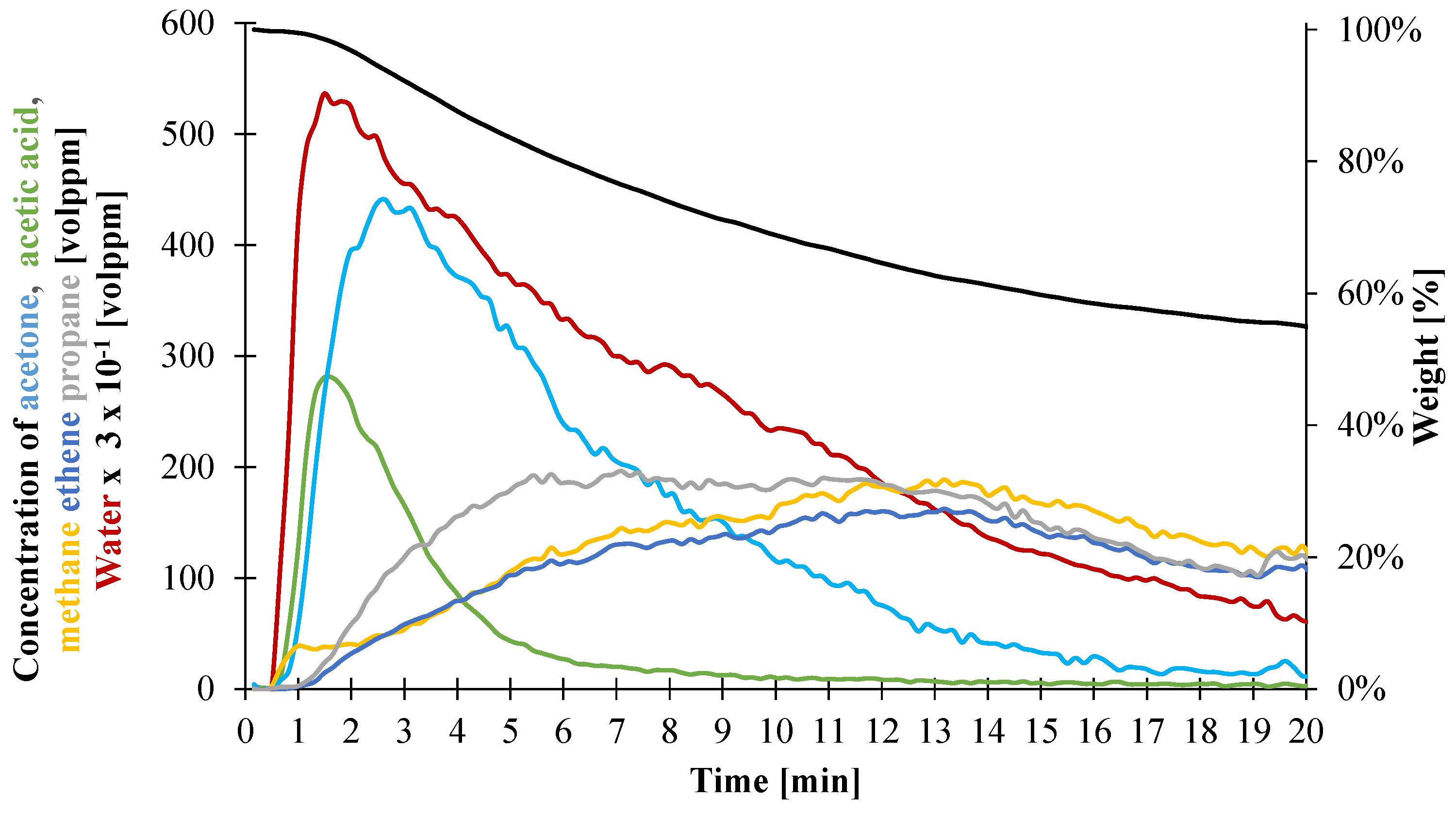
3.1.4. Determination of Heat Capacity of the Decomposition Gases

| Gas1 | Gas2 | |||||
|---|---|---|---|---|---|---|
| Acetic Acid | Acetone | Water | Ethene | Propane | Methane | |
| Total Gas Evolved (vol. ppm) | 837 | 2936 | 151,337 | 2588 | 3110 | 3017 |
| Mass ratio of evolved gases | 2.0 × 10⁻² | 6.0 × 10⁻² | 1.0 | 1.5 | 2.8 | 1.0 |
| Composition in individual gas (wt %) | 1.7 | 5.8 | 92.5 | 28.1 | 53.1 | 18.8 |

3.1.5. Determination of the Optical Properties


3.1.6. Conclusion about the Characterization of the Inputs Data
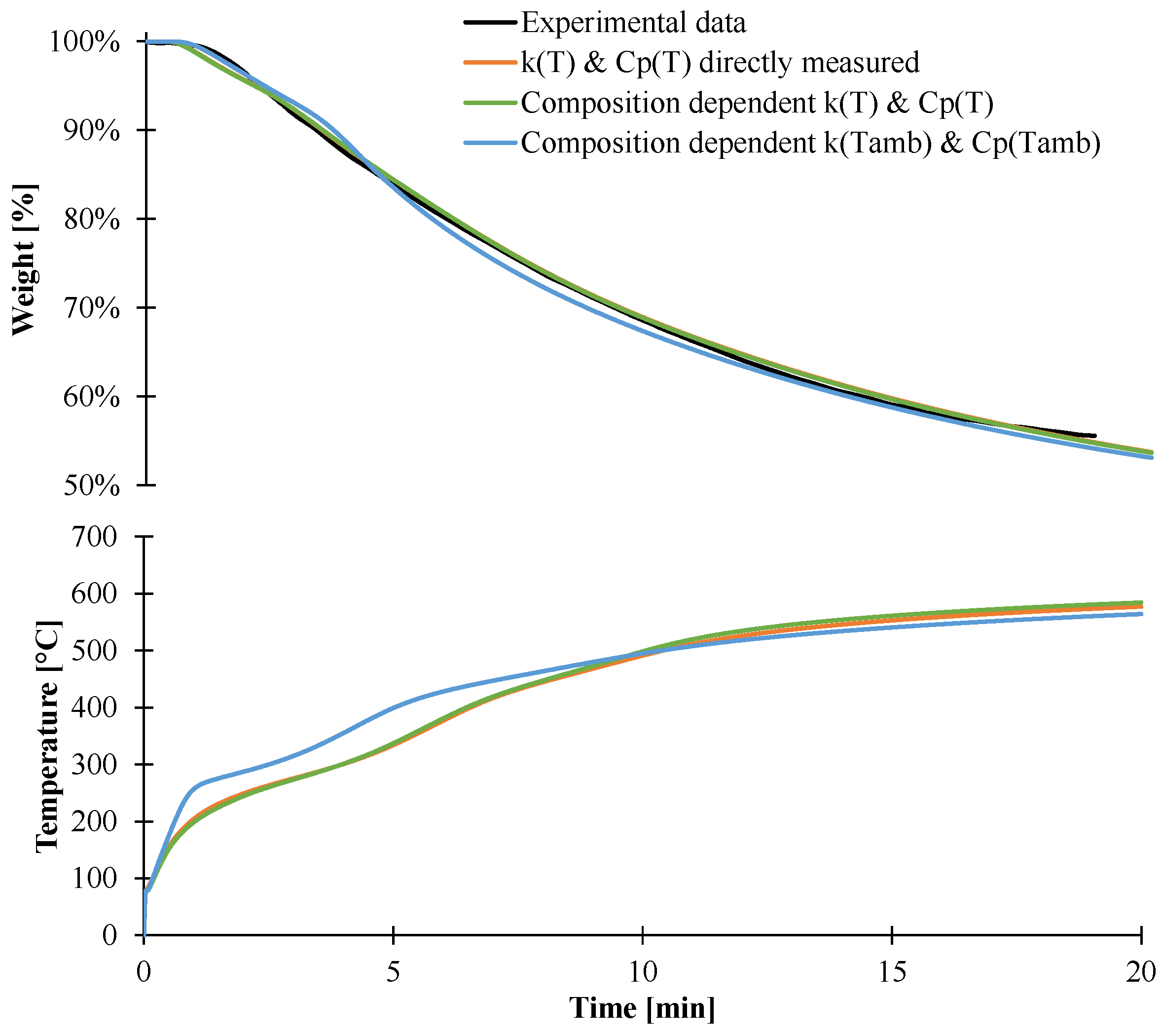
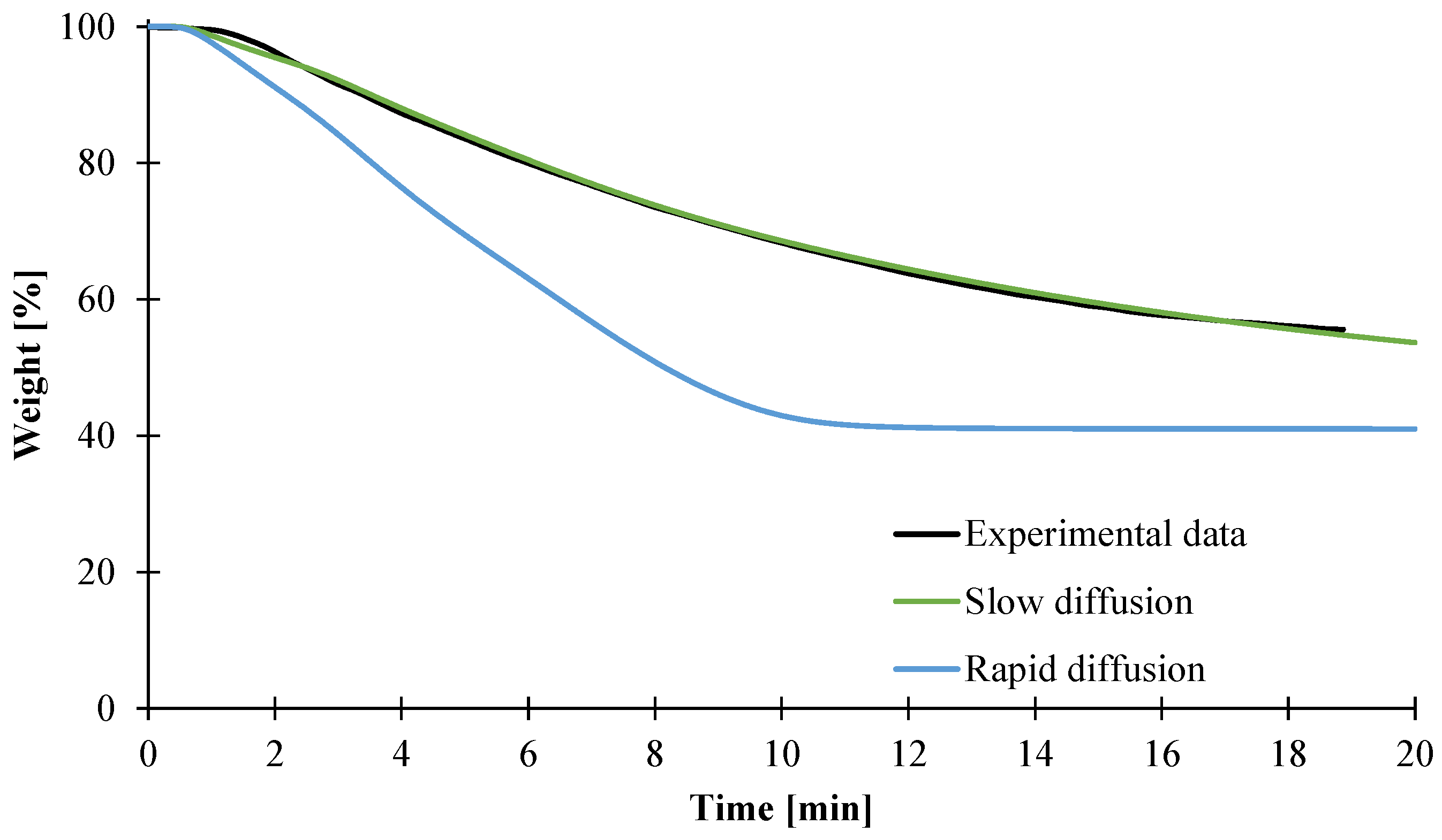
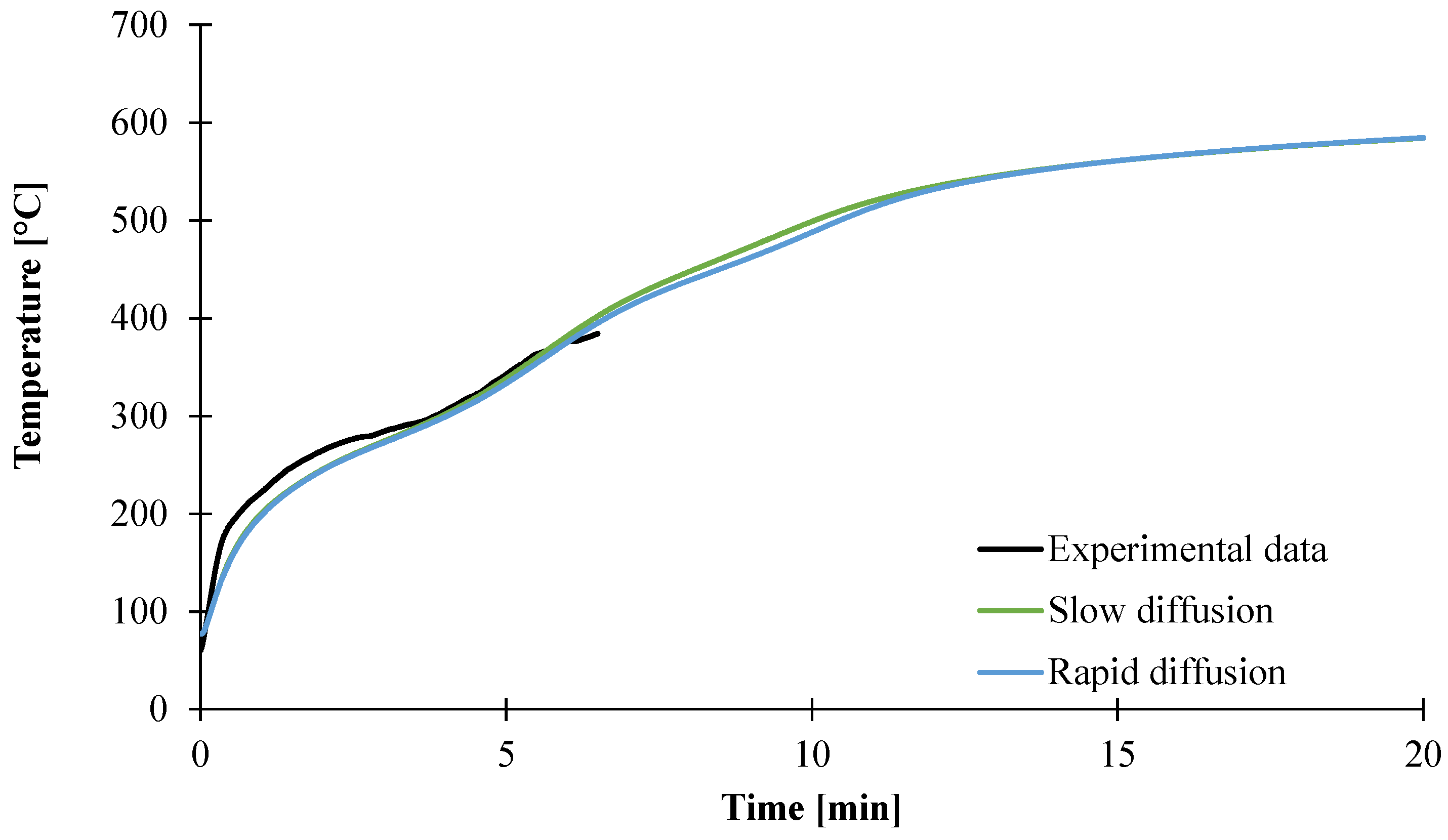
3.2. Modeling of the Gasification of EVA/ATH

4. Conclusions
Acknowledgments
Author Contributions
Conflicts of Interest
Nomenclature
| General parameters/variables | |||
| t | Time | x | Depth |
| T | Temperature | m | Mass |
| Nr | Number of decomposition reactions of the material | Ng | Number of gaseous component released by the material |
| Optical properties | |||
| M | Black body excitance | I | Irradiance |
| α | Reflectivity | A | Absorption coefficient |
| ε | Emissivity | T | Transmittance |
| λ | Wavelength | R | Reflectance |
| d | Thickness | ||
| Kinetic parameters | |||
| Reaction rate for reaction r | R | Ideal gas constant | |
| Ar | Pre-exponential factor | n | Order of reaction |
| Er | Activation energy for reaction r | Stoichiometric coefficient of component i in reaction r | |
| Thermo-physical properties | |||
| Cp | Heat capacity | ρ | Density |
| k | Thermal conductivity | Hr | Enthalpy of reaction r |
| Dgas i | Mass trans transfer coefficient of component i | ||
References
- McGrattan, K.; Hostikka, S.; McDermott, R.; Floyd, J.; Weinschenk, C.; Overholt, K. Fire Dynamics Simulator (version 6) User’s Guide; National Institute of Standards and Technology: Gaithersburg, MD, USA, 2013; Special Publication 1019. [Google Scholar]
- Lautenberger, C.; Fernandez-Pello, C. Generalized pyrolysis model for combustible solids. Fire Saf. J. 2009, 44, 819–839. [Google Scholar] [CrossRef]
- Stoliarov, S.I.; Lyon, R.E. Thermo-Kinetic Model of Burning for Pyrolyzing Materials; Federal Aviation Administration: Washington, DC, USA, 2008. [Google Scholar]
- Snegirev, A.Y.; Talalov, V.A.; Stepanov, V.V.; Harris, J.N. A new model to predict pyrolysis, ignition and burning of flammable materials in fire tests. Fire Saf. J. 2013, 59, 132–150. [Google Scholar] [CrossRef]
- Shi, L.; Yit Lin Chew, M. A review of fire processes modeling of combustible materials under external heat flux. Fuel 2013, 106, 30–50. [Google Scholar] [CrossRef]
- Janssens, M. Fundamental Thermophysical Characteristics of Wood and Their Role in Enclosure Fire Growth; Ghent University: Ghent, Belgium, 1991. [Google Scholar]
- Janssens, M. Piloted Ignition of Wood. Fire Mater. 1991, 15, 151–167. [Google Scholar] [CrossRef]
- Staggs, J.E.J.; Nelson, M.I. A critical mass flux model for the flammability of thermoplastics. Combust. Theory Model. 2001, 5, 399–427. [Google Scholar] [CrossRef]
- Di Blasi, C. Modeling and simulation of combustion processes of charring and non-charring solid fuels. Prog. Energy Combust. Sci. 1993, 19, 71–104. [Google Scholar] [CrossRef]
- Nelson, M.I.; Brindley, J.; McIntosh, A.C. The dependence of critical heat flux on fuel and additive properties: A critical mass flux model. Fire Saf. J. 1995, 24, 107–130. [Google Scholar] [CrossRef]
- Babrauskas, V.; Twilley, W.H.; Janssens, M.; Yusa, S. A cone calorimeter for controlled-atmosphere studies. Fire Mater. 1991, 16, 37–43. [Google Scholar] [CrossRef]
- Chaos, M.; Khan, M.M.; Krishnamoorthy, N.; de Ris, J.L.; Dorofeev, S.B. Evaluation of optimization schemes and determination of solid fuel properties for CFD fire models using bench-scale pyrolysis tests. Proc. Combust. Inst. 2011, 33, 2599–2606. [Google Scholar] [CrossRef]
- Li, J.; Gong, J.; Stoliarov, S.I. Gasification experiments for pyrolysis model parameterization and validation. Int. J. Heat Mass Transf. 2014, 77, 738–744. [Google Scholar] [CrossRef]
- ASTM E2716–09 Standard Test Method for Entahlpies of Fusion and Crystallization by Diffential Scanning Calorimetry; ASTM International: West Conshohocken, PA, USA, 2012.
- ASTM E2585–09 Standard Practice fo Thermal Diffusivity By the Flash Method; ASTM International: West Conshohocken, PA, USA, 2012.
- ASTM E1269–11 Standard Test Method for Determining Specific Heat Capacity by Differential Scanning Calorimetry; ASTM International: West Conshohocken, PA, USA, 2012.
- ISO 11357–4 Plastics—Differential Scanning Calorimetry (DSC)—Part 4: Determination of Specific Heat Capacity; ISO: Geneva, Switzerland, 2014.
- ISO 22007–2 Plastics—Determination of Thermal Conductivity and Thermal Diffusivity—Part 2: Transient Plane Heat Source (Hot Disc) Method; ISO: Geneva, Switzerland, 2008.
- Witkowski, A.; Girardin, B.; Försth, M.; Hewitt, F.; Fontaine, G.; Duquesne, S.; Bourbigot, S.; Hull, T.R. Development of an anaerobic pyrolysis model for fire retardant cable sheathing materials. Polym. Degrad. STable 2015, 113, 208–217. [Google Scholar] [CrossRef]
- Li, J.; Stoliarov, S.I. Measurement of kinetics and thermodynamics of the thermal degradation for charring polymers. Polym. Degrad. Stabil. 2014, 106, 2–15. [Google Scholar] [CrossRef]
- Li, J.; Stoliarov, S.I. Measurement of kinetics and thermodynamics of the thermal degradation for non-charring polymers. Combust. Flame 2013, 160, 1287–1297. [Google Scholar] [CrossRef]
- Kempel, F.; Schartel, B.; Linteris, G.T.; Stoliarov, S.I.; Lyon, R.E.; Walters, R.N.; Hofmann, A. Prediction of the mass loss rate of polymer materials: Impact of residue formation. Combust. Flame 2012, 159, 2974–2984. [Google Scholar] [CrossRef]
- Mhike, W.; Ferreira, I.V.W.; Li, J.; Stoliarov, S.I.; Focke, W.W. Flame retarding effect of graphite in rotationally molded polyethylene/graphite composites. J. Appl. Polym. Sci. 2015, 132. [Google Scholar] [CrossRef]
- Chase, M.W., Jr. NIST-JANAF Themochemical Tables, 4th ed.; Series Journal of Physical and Chemical Reference Data, No. 9; American Chemical Society: Washington, DC, USA; American Institute of Physics for the National Institute of Standards and Technology: Washington, DC, USA, 1998; p. 1951. [Google Scholar]
- Ginnings, D.C.; Corruccini, R.J. Enthalpy, specific heat, and entropy of aluminum oxide from 0 to 900 °C. J. Res. Natl. Bur. Stand. 1947, 38, 593–600. [Google Scholar] [CrossRef]
- Beyer, G. Flame Retardancy of Nanocomposites—From Research to Technical Products. J. Fire Sci. 2005, 23, 75–87. [Google Scholar] [CrossRef]
- Rothon, R.; Hornsby, P. Fire Retardants Fillers for Polymers. In Polymer Green Flame Retardants; Elsevier: Amsterdam, The Netherlands, 2014; pp. 289–321. [Google Scholar]
- Beyer, G. Flame retardancy of nanocomposites based on organoclays and carbon nanotubes with aluminium trihydrate. Polym. Adv. Technol. 2006, 17, 218–225. [Google Scholar] [CrossRef]
- Srivastava, S.K.; Kuila, T. Fire Retardancy of Elastomers and Elastomer Nanocompistes. In Polymer Green Flame Retardants; Elsevier: Amsterdam, The Netherlands, 2014; pp. 597–651. [Google Scholar]
- Opfermann, J.R. Kinetic Analysis Using Multivariate Non-linear Regression. I. Basic concepts. J. Therm. Anal. Calorim. 2000, 60, 641–658. [Google Scholar] [CrossRef]
- Opfermann, J.R.; Kaisersberger, E.; Flammersheim, H.J. Model-free analysis of thermoanalytical data-advantages and limitations. Thermochim. Acta 2002, 391, 119–127. [Google Scholar] [CrossRef]
- Cérin, O.; Duquesne, S.; Fontaine, G.; Roos, A.; Bourbigot, S. Thermal degradation of elastomeric vulcanized poly(ethylene-co-vinyl acetate) (EVM): Chemical and kinetic investigations. Polym. Degrad. Stabil. 2011, 96, 1812–1820. [Google Scholar] [CrossRef]
- Boulet, P.; Parent, G.; Acem, Z.; Collin, A.; Försth, M.; Bal, N.; Rein, G.; Torero, J. Radiation emission from a heating coil or a halogen lamp on a semitransparent sample. Int. J. Therm. Sci. 2014, 77, 223–232. [Google Scholar] [CrossRef]
- Försth, M.; Roos, A. Absorptivity and its dependence on heat source temperature and degree of thermal breakdown. Fire Mater. 2011, 35, 285–301. [Google Scholar] [CrossRef]
- Boulet, P.; Gérardin, J.; Acem, Z.; Parent, G.; Collin, A.; Pizzo, Y.; Porterie, B. Optical and radiative properties of clear PMMA samples exposed to a radiant heat flux. Int. J. Therm. Sci. 2014, 82, 1–8. [Google Scholar] [CrossRef]
- Stoliarov, S.I.; Crowley, S.; Lyon, R.E.; Linteris, G.T. Prediction of the burning rates of non-charring polymers. Combust. Flame 2009, 156, 1068–1083. [Google Scholar] [CrossRef]
- Staggs, J.E.J.; Whiteley, R.H. Modelling the combustion of solid-phase fuels in cone calorimeter experiments. Fire Mater. 1999, 23, 63–69. [Google Scholar] [CrossRef]
- Quintiere, J.G.; Liu, X. Flammability Properties of Clay-Nylon Nanocomposites; Federal Aviation Administration: Washington, DC, USA, 2004. [Google Scholar]
- Rimez, B.; Rahier, H.; Van Assche, G.; Artoos, T.; Van Mele, B. The thermal degradation of poly(vinyl acetate) and poly(ethylene-co-vinyl acetate), Part II: Modelling the degradation kinetics. Polym. Degrad. Stabil. 2008, 93, 1222–1230. [Google Scholar] [CrossRef]
- Rimez, B.; Rahier, H.; Van Assche, G.; Artoos, T.; Biesemans, M.; Van Mele, B. The thermal degradation of poly(vinyl acetate) and poly(ethylene-co-vinyl acetate), Part I: Experimental study of the degradation mechanism. Polym. Degrad. Stabil. 2008, 93, 800–810. [Google Scholar] [CrossRef]
- Costache, M.C.; Jiang, D.D.; Wilkie, C.A. Thermal degradation of ethylene–vinyl acetate coplymer nanocomposites. Polymer (Guildf) 2005, 46, 6947–6958. [Google Scholar] [CrossRef]
- Witkowski, A.; Stec, A.A.; Hull, T.R.; Richard Hull, T. The influence of metal hydroxide fire retardants and nanoclay on the thermal decomposition of EVA. Polym. Degrad. STable 2012, 97, 2231–2240. [Google Scholar] [CrossRef]
- Wang, X.; Rathore, R.; Songtipya, P.; del Mar Jimenez-Gasco, M.; Manias, E.; Wilkie, C.A. EVA-layered double hydroxide (nano)composites: Mechanism of fire retardancy. Polym. Degrad. Stabil. 2011, 96, 301–313. [Google Scholar] [CrossRef]
- Patel, M.; Pitts, S.; Beavis, P.; Robinson, M.; Morrell, P.; Khan, N.; Khan, I.; Pockett, N.; Letant, S.; Von White, G.; Labouriau, A. Thermal stability of poly(ethylene-co-vinyl acetate) based materials. Polym. Test. 2013, 32, 785–793. [Google Scholar] [CrossRef]
- Hoffendahl, C.; Fontaine, G.; Duquesne, S.; Taschner, F.; Mezger, M.; Bourbigot, S. The combination of aluminum trihydroxide (ATH) and melamine borate (MB) as fire retardant additives for elastomeric ethylene vinyl acetate (EVA). Polym. Degrad. Stabil. 2015, 115, 77–88. [Google Scholar] [CrossRef]
- Stoliarov, S.I.; Crowley, S.; Walters, R.N.; Lyon, R.E. Prediction of the burning rates of charring polymers. Combust. Flame 2010, 157, 2024–2034. [Google Scholar] [CrossRef]
- Ngohang, F.-E.; Fontaine, G.; Gay, L.; Bourbigot, S. Smoke composition using MLC/FTIR/ELPI: Application to flame retarded ethylene vinyl acetate. Polym. Degrad. Stabil. 2015, 115, 89–109. [Google Scholar] [CrossRef]
- Luche, J.; Mathis, E.; Rogaume, T.; Richard, F.; Guillaume, E. High-density polyethylene thermal degradation and gaseous compound evolution in a cone calorimeter. Fire Saf. J. 2012, 54, 24–35. [Google Scholar] [CrossRef]
- Lemmon, E.W.; McLinden, L.O.; Friend, D.G. In Thermophysical Properties of Fluid Systems; NIST Chemistry WebBook, reference database 69. Available online: http://webbook.nist.gov/chemistry/ (accessed on 10 October 2015).
- Li, J.; Gong, J.; Stoliarov, S.I. Development of pyrolysis models for charring polymers. Polym. Degrad. Stabil. 2015, 115, 138–152. [Google Scholar] [CrossRef]
- Wasan, S.R.; Rauwoens, P.; Vierendeels, J.; Merci, B. Application of a simple enthalpy-based pyrolysis model in numerical simulations of pyrolysis of charring materials. Fire Mater. 2009. [Google Scholar] [CrossRef] [Green Version]
- Hasan, M.A.; Zaki, M.I.; Pasupulety, L. Oxide-catalyzed conversion of acetic acid into acetone: An FTIR spectroscopic investigation. Appl. Catal. A Gen. 2003, 243, 81–92. [Google Scholar] [CrossRef]
- Pei, Z.-F.; Ponec, V. On the intermediates of the acetic acid reactions on oxides: An IR study. Appl. Surf. Sci. 1996, 103, 171–182. [Google Scholar] [CrossRef]
- Martinez, R. Ketonization of acetic acid on titania-functionalized silica monoliths. J. Catal. 2004, 222, 404–409. [Google Scholar] [CrossRef]
- Statler, D.L.; Gupta, R.K. A Finite Element Analysis on the Modeling of Heat Release Rate, as Assessed by a Cone Calorimeter of Char Forming Polycarbonate. In Proceedings of the COMSOL Conference, Boston, MA, USA, 9–11 October 2008.
© 2015 by the authors; licensee MDPI, Basel, Switzerland. This article is an open access article distributed under the terms and conditions of the Creative Commons by Attribution (CC-BY) license (http://creativecommons.org/licenses/by/4.0/).
Share and Cite
Girardin, B.; Fontaine, G.; Duquesne, S.; Försth, M.; Bourbigot, S. Characterization of Thermo-Physical Properties of EVA/ATH: Application to Gasification Experiments and Pyrolysis Modeling. Materials 2015, 8, 7837-7863. https://doi.org/10.3390/ma8115428
Girardin B, Fontaine G, Duquesne S, Försth M, Bourbigot S. Characterization of Thermo-Physical Properties of EVA/ATH: Application to Gasification Experiments and Pyrolysis Modeling. Materials. 2015; 8(11):7837-7863. https://doi.org/10.3390/ma8115428
Chicago/Turabian StyleGirardin, Bertrand, Gaëlle Fontaine, Sophie Duquesne, Michael Försth, and Serge Bourbigot. 2015. "Characterization of Thermo-Physical Properties of EVA/ATH: Application to Gasification Experiments and Pyrolysis Modeling" Materials 8, no. 11: 7837-7863. https://doi.org/10.3390/ma8115428