Multi-Echo-Based Echo-Planar Spectroscopic Imaging Using a 3T MRI Scanner

Abstract
:1. Introduction
2. Theory
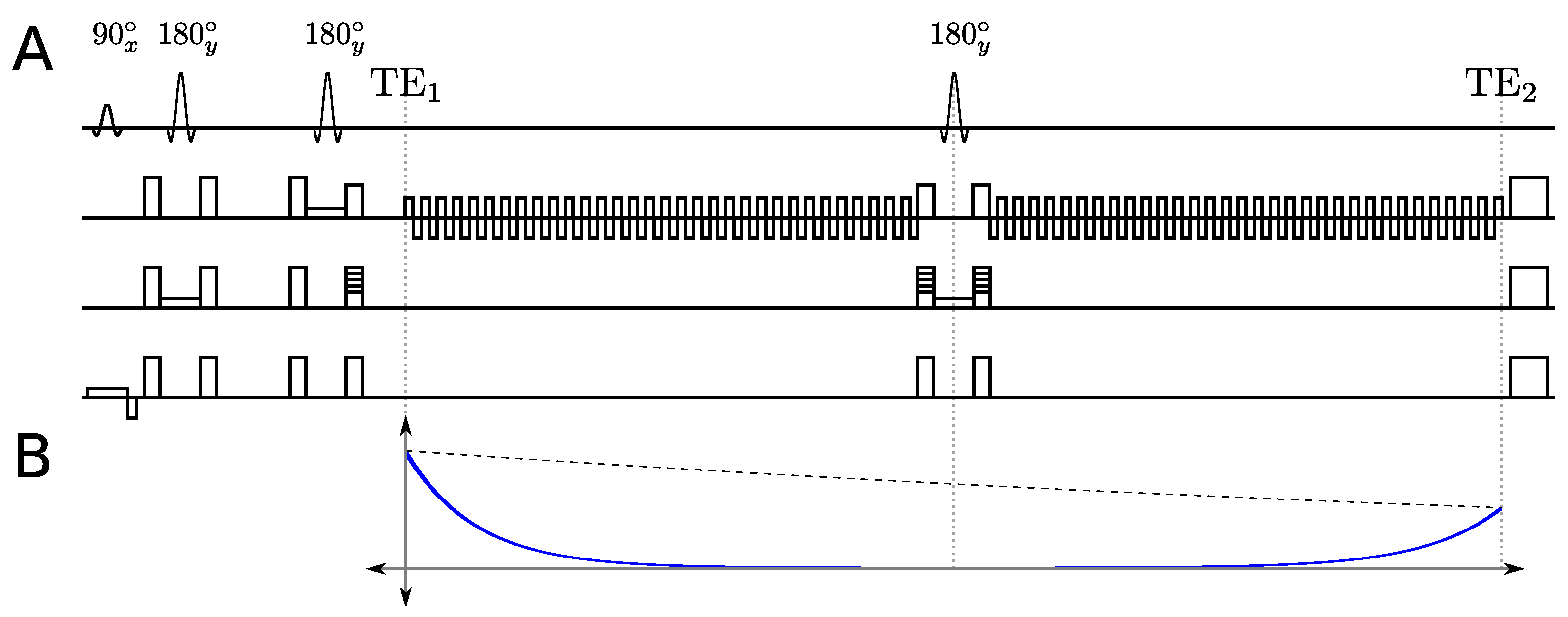
2.1. Multi-Echo Sequence

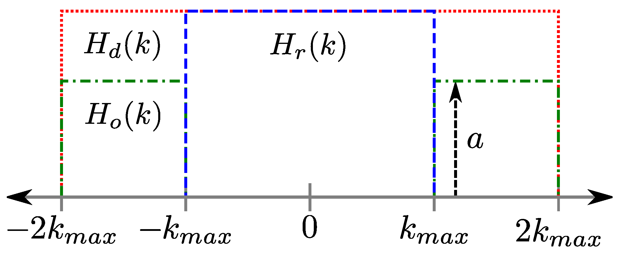
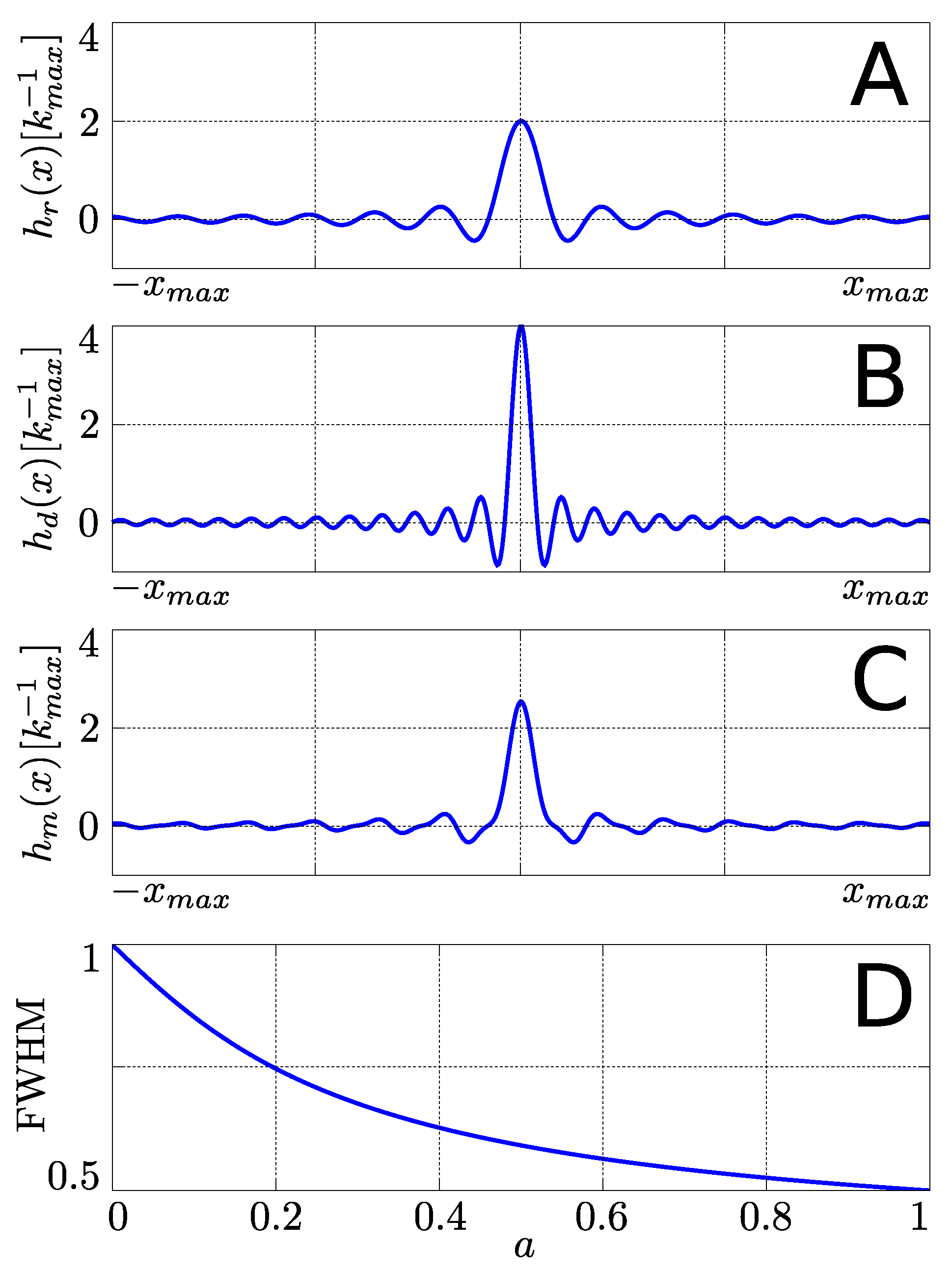
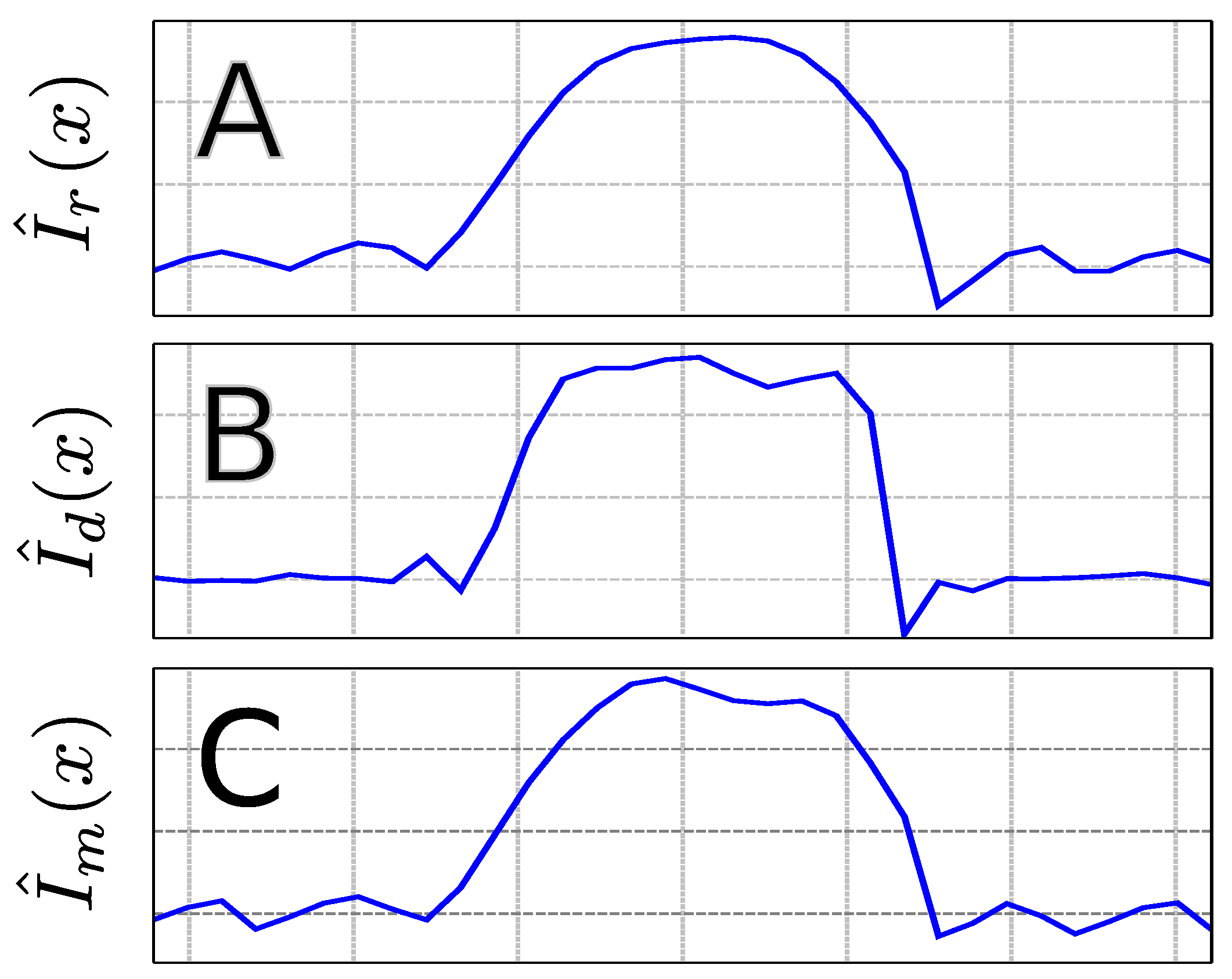
2.2. Multi-Echo PSFs


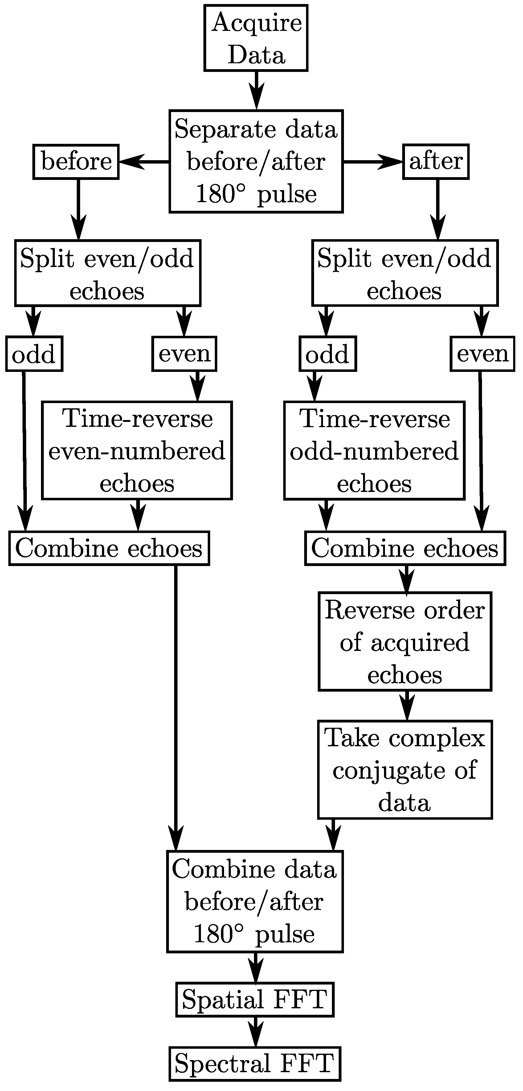
3. Methods

| Scan | Grid | Voxel Size | Readout Points | Scan Time |
|---|---|---|---|---|
| 4 cm | 512 | 1 m 42 s | ||
| 2 cm | 512 | 3 m 18 s | ||
| 2 cm | 256 | 1 m 42 s |
| Scan | Readout Points | Scan Time | |
|---|---|---|---|
| 512 | N/A | 4 m 54 s | |
| 256 | 442.5 ms | 2 m 30 s | |
| 128 | 227.5 ms | 2 m 30 s | |
| 64 | 120 ms | 2 m 30 s |
4. Results
4.1. Phantom Scans

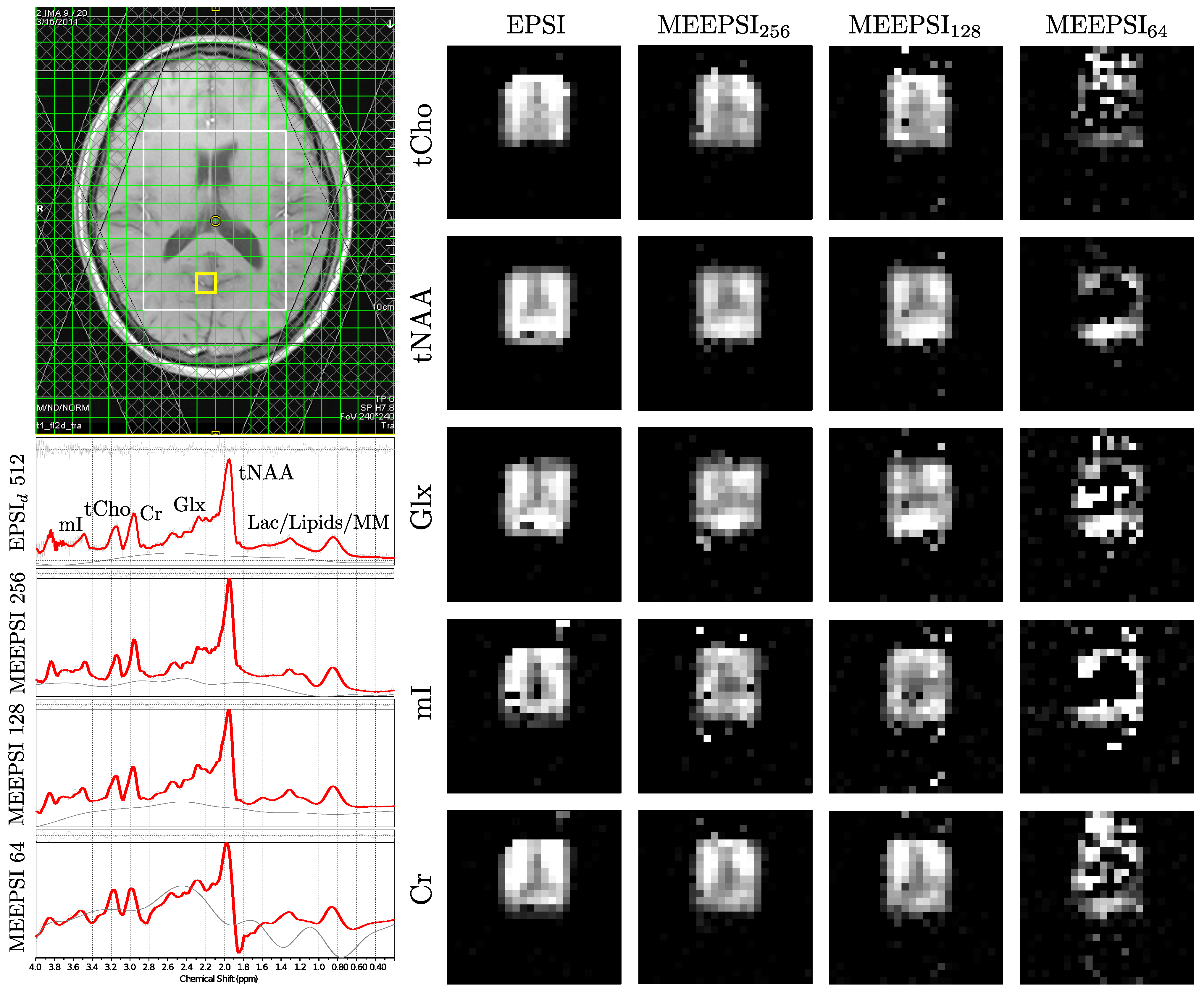
4.2. In Vivo Scans

| Mean Ratio | CV(%) | Mean Ratio | CV(%) | Mean Ratio | CV(%) | Mean Ratio | CV(%) | |||||
|---|---|---|---|---|---|---|---|---|---|---|---|---|
| NAA | 2.093 | 31.7 | 48 | 1.879 | 28.3 | 48 | 1.987 | 26.3 | 48 | 2.146 | 39.3 | 22 |
| Glu | 1.339 | 38.1 | 38 | 1.295 | 34.2 | 48 | 1.448 | 34.4 | 46 | 2.623 | 48.7 | 17 |
| GSH | 0.316 | 21.1 | 8 | 0.296 | 28.4 | 43 | 0.298 | 25.8 | 23 | 1.269 | 55.8 | 9 |
| mI | 0.631 | 31.4 | 37 | 0.726 | 27.2 | 47 | 0.681 | 26.7 | 47 | 2.401 | 90.6 | 20 |
| tCho | 0.338 | 17.5 | 47 | 0.310 | 20.8 | 48 | 0.341 | 43.4 | 47 | 0.334 | 76.2 | 25 |
| tNAA | 2.139 | 33.0 | 48 | 1.918 | 27.5 | 48 | 2.003 | 27.2 | 48 | 2.420 | 49.4 | 27 |
| Glx | 1.964 | 33.8 | 45 | 1.740 | 35.1 | 48 | 1.801 | 40.8 | 46 | 2.605 | 45.1 | 22 |
5. Discussion
| NAA, ms | Cr (3.03), ms | Cr (3.92), ms | Cho, ms | ||||||
|---|---|---|---|---|---|---|---|---|---|
| a | a | a | a | ||||||
| 442.5 ms | 0.20 | ∼50% | 0.05 | ∼15% | 0.03 | ∼10% | 0.10 | ∼29% | |
| 227.5 ms | 0.44 | ∼77% | 0.22 | ∼53% | 0.17 | ∼44% | 0.31 | ∼65% | |
| 120.0 ms | 0.65 | ∼89% | 0.45 | ∼78% | 0.39 | ∼73% | 0.54 | ∼84% | |
6. Conclusions
Acknowledgements
References
- Brown, T.; Kincaid, B.; Ugurbil, K. NMR chemical shift imaging in three dimensions. Proc. Natl. Acad. Sci. USA 1982, 79, 3523–3526. [Google Scholar] [CrossRef]
- Maudsley, A.; Hilal, S.; Perman, W.; Simon, H. Spatially resolved high resolution spectroscopy by four-dimensional NMR. J. Magn. Reson. 1983, 51, 147–152. [Google Scholar]
- Mansfield, P. Spatial mapping of the chemical shift in NMR. J. Phys. D Appl. Phys. 1983, 16, L235–L238. [Google Scholar] [CrossRef]
- Mansfield, P. Spatial mapping of the chemical shift in NMR. Magn. Reson. Med. 1984, 1, 370–386. [Google Scholar] [CrossRef] [PubMed]
- Matsui, S.; Sekihara, K.; Kohno, H. Spatially resolved NMR spectroscopy using phase-modulated spin-echo trains. J. Magn. Reson. 1986, 67, 476–490. [Google Scholar]
- Posse, S.; DeCarli, C.; Le-Bihan, D. 3D echo planar spectroscopic imaging at short echo times in human brain. Radiology 1994, 192, 733–738. [Google Scholar]
- Posse, S.; Tedeschi, G.; Risinger, R.; Ogg, R.; Le-Bihan, D. High speed 1H spectroscopic imaging in human brain by echo planar spatial-spectral encoding. Magn. Reson. Med. 1995, 33, 34–40. [Google Scholar] [CrossRef]
- Ebel, A.; Soher, B.; Maudsley, A. Assessment of 3D proton mr echoplanar spectroscopic imaging using automated spectral analysis. Magn. Reson. Med. 2001, 46, 1072–1078. [Google Scholar] [CrossRef] [PubMed]
- Lipnick, S.; Verma, G.; Ramadan, S.; Furuyama, J.; Thomas, M. Echo planar correlated spectroscopic imaging: Implementation and pilot evaluation in human calf in vivo. Magn. Reson. Med. 2010, 64, 947–956. [Google Scholar] [CrossRef] [PubMed]
- Duyn, J.; Moonen, C. Fast proton spectroscopic imaging of human brain using multiple spin-echoes. Magn. Reson. Med. 1993, 30, 409–414. [Google Scholar] [CrossRef]
- Dreher, W.; Leibfritz, D. Fast proton spectroscopic imaging with high signal-to-noise ratio: Spectroscopic RARE. Magn. Reson. Med. 2002, 47, 523–528. [Google Scholar] [CrossRef] [PubMed]
- Mulkern, R.; Chao, H.; Bowers, J.; Holtzman, D. Multiecho approaches to spectroscopic imaging of the brain. Ann. N. Y. Acad. Sci. 1997, 30, 97–122. [Google Scholar] [CrossRef]
- Provencher, S. Estimation of metabolite concentrations from localized in vivo proton NMR spectra. Magn. Reson. Med. 1993, 30, 672–679. [Google Scholar] [CrossRef] [PubMed]
- Mulkern, R.; Panych, L. Echo planar spectroscopic imaging. Concepts Magn. Reson. 2001, 13, 213–237. [Google Scholar] [CrossRef]
- Bottomley, P. Spatial localization in NMR Spectroscopy in vivo. Ann. N. Y. Acad. Sci. 1987, 508, 333–348. [Google Scholar] [CrossRef] [PubMed]
- Frahm, J.; Merboldt, K.; Hanicke, W.; Haase, A. Stimulated echo imaging. J. Magn. Reson. 1985, 64, 81–93. [Google Scholar]
- Yahya, A.; Fallone, B. Detection of glutamate and glutamine (Glx) by turbo spectroscopic imaging. J. Magn. Reson. 2009, 196, 170–177. [Google Scholar] [CrossRef] [PubMed]
- Ogg, R.; Kingsley, P.; Taylor, J. WET, a T1 and B1 insensitive water-suppression method for in vivo localized 1H NMR spectroscopy. J. Magn. Reson. B 1994, 104, 1–10. [Google Scholar] [CrossRef] [PubMed]
- Klose, U. In vivo proton spectroscopy in presence of eddy currents. Magn. Reson. Med. 1990, 14, 26–30. [Google Scholar] [CrossRef] [PubMed]
- Günther, U.; Ludwig, C.; Rüterjans, H. WAVEWAT—Improved solvent suppression in NMR spectra employing wavelet transforms. J. Magn. Reson 2002, 156, 19–25. [Google Scholar] [CrossRef]
- Smith, S.; Levante, T.; Meier, B.; Ernst, R. Computer simulations in magnetic resonance. An object-oriented programming approach. J. Magn. Reson. 1994, 106a, 75–105. [Google Scholar]
- Liang, Z.; Lauterbur, P. Principles of Magnetic Resonance Imaging: A Signal Processing Perspective; Wiley-IEEE Press: New York, NY, USA, 1999. [Google Scholar]
- Cavassila, S.; Deval, S.; Huegen, C.; van Ormondt, D.; Graveron-Demilly, D. Cramér-Rao bounds: An evaluation tool for quantitation. NMR Biomed. 2001, 14, 278–283. [Google Scholar] [CrossRef] [PubMed]
- Becker, E.; Ferretti, J.; Gambhir, P. Selection of optimum parameters for pulse fourier transform nuclear magnetic resonance. Anal. Chem. 1979, 51, 1413–1420. [Google Scholar] [CrossRef]
- Mlynarik, V.; Gruber, S.; Moser, E. Proton T1 and T2 relaxation times of human brain metabolites at 3 Tesla. NMR Biomed. 2001, 14, 325–331. [Google Scholar] [CrossRef] [PubMed]
© 2011 by the authors; licensee MDPI, Basel, Switzerland. This article is an open access article distributed under the terms and conditions of the Creative Commons Attribution license (http://creativecommons.org/licenses/by/3.0/.)
Share and Cite
Furuyama, J.K.; Burns, B.L.; Wilson, N.E.; Thomas, M.A. Multi-Echo-Based Echo-Planar Spectroscopic Imaging Using a 3T MRI Scanner. Materials 2011, 4, 1818-1834. https://doi.org/10.3390/ma4101818
Furuyama JK, Burns BL, Wilson NE, Thomas MA. Multi-Echo-Based Echo-Planar Spectroscopic Imaging Using a 3T MRI Scanner. Materials. 2011; 4(10):1818-1834. https://doi.org/10.3390/ma4101818
Chicago/Turabian StyleFuruyama, Jon K., Brian L. Burns, Neil E. Wilson, and M. Albert Thomas. 2011. "Multi-Echo-Based Echo-Planar Spectroscopic Imaging Using a 3T MRI Scanner" Materials 4, no. 10: 1818-1834. https://doi.org/10.3390/ma4101818