High-Resolution Wave Energy Assessment in Shallow Water Accounting for Tides

Abstract

The wave energy in a shallow water location is evaluated considering the influence of the local tide and wind on the wave propagation. The target is the coastal area just north of the Portuguese city of Peniche, where a wave energy converter operates on the sea bottom. A wave modelling system based on SWAN has been implemented and focused on this coastal environment in a multilevel computational scheme. The first three SWAN computational belonging to this wave prediction system were defined using the spherical coordinates. In the highest resolution computational domain, Cartesian coordinates have been considered, with a resolution of 25 m in both directions. An in-depth analysis of the main characteristics of the environmental matrix has been performed. This is based on the results of eight-year model system simulations (2005–2012). New simulations have been carried out in the last two computational domains with the most relevant wave and wind patterns, considering also the tide effect. The results show that the tide level, together with the wind intensity and direction, may influence to a significant degree the wave characteristics. This especially concerns the wave power in the location where the wave converter operates.

1. Introduction

Wave energy represents at this moment the largest untapped form of renewable energy in the world. Ocean waves are consistent and sea states can be accurately predicted usually more than 48 h in advance. Besides predictability, another factor that makes wave energy particularly attractive for electricity generation, compared to the power density of solar or wind energy, is its high power density. This is the power per meter of wave front. From this perspective, in future decades, ocean waves are expected to produce at least 10% of the global energy demand [1]. Moreover, by 2050, the electric power delivered by wave energy farms could exceed the global installed capacity of wind and solar power together [2].

The combination of the Earth’s rotation and the westerly direction of the prevailing winds induces a high level of wave energy resources along the western coasts of the continents. This is especially true for locations where waves can travel without obstacles for thousands of miles. The coastal environment of continental Portugal satisfies these conditions [3,4,5], since it is the westernmost country of Europe and is bordered on its west side by the Atlantic Ocean. That is why in recent years this nearshore has captured the interest of wave energy developers for implementing pioneering projects [6].

The area of the present study, located north of Peniche, has a special feature that is caused by the vicinity of the Nazaré Canyon. This is the biggest underwater ravine in Europe. It runs 125 miles from the abyssal plain out into the Atlantic Ocean less than half a mile from the coastline. At its deepest point, the sea bed is more than 3 miles beneath the surface and it rises rapidly to a canyon “headwall”. Thus, in the case of the Nazaré canyon, the fact that its head is situated near the shore causes a significant influence on the hydrodynamic and sediment transport processes. This leads to particular oceanographic conditions, intrinsically connected with its morphology. It has to be highlighted that only a few miles north from this area is Praia do Norte, near the fishing village of Nazaré. At that location the waves are famed for being among the largest in the world [7]. In this particular coastal area, the currents through the canyon combine with the swell driven by the wind from further out in the Atlantic. They converge as the canyon narrows and drive the swell directly towards the lighthouse that sits on the edge of Nazaré.

The wave height is influenced, among others factors, by the tidal conditions, due to wave–current interactions. A hindcast study has been conducted by Sebastião et al. [8] to determine the time history of the water level at the Portuguese coast resulting from tides and storm surges. Other studies have also addressed the modelling of tides at the Portuguese coast as well as the induced tidal currents [9,10]. They show that the area north of Peniche is a site of intensified currents.

The WaveRoller device is installed near Peniche [11,12] in a water depth of around 15 m. This area is located about 75 miles north of Lisbon and was identified as having high wave conditions [13]. After almost a decade of R&D in wave energy and after testing the prototype WaveRoller at the real scale at EMEC in Scotland and in Portugal, a second prototype was installed and tested in the Portuguese seas. It is a nearshore technology, designed to operate at a depth between 8–20 m and fixed at the sea bottom. It uses the horizontal movement of the waves at low depth to move its vertical wings. The WaveRoller device is in fact a vertical plate rotating an axis located at the bottom edge of the plate. The back and forth movement of bottom waves moves the plate and the motion produced moves a piston. This energy is further converted into electricity by a hydraulic system in combination with a hydraulic motor/generator device [14].

Following extended marine trials of the WaveRoller prototypes in Peniche in 2007 and 2008, the wave energy farm consisted of three 100 kW WaveRoller units (total nominal capacity of the farm 300 kW). They were deployed in 2012 and are still in operation.

The main objective of the present work is to evaluate the influence on the wave conditions of some other components of the environment in the coastal area where the WaveRoller farm operates. This especially concerns the tide and the wind.

2. Wave Modelling in the Portuguese Nearshore

Nowadays, spectral phase-averaged wave models are among the most appropriate tools for providing reliable information related to wave conditions on large geographical spaces. For this purpose, some previous studies were performed in Centre for Marine Technology and Ocean Engineering (CENTEC). These consider a wave prediction system based on WAM (Wave Model) [15], for the wave generation and propagation at the level of the entire North Atlantic Ocean, and SWAN (Simulating Waves Nearshore) [16], for the wave transformation at the level of the western side of the Iberian Peninsula [17,18]. This system was subsequently focused on the most relevant coastal areas, such as the Portuguese harbours [19,20]. At the same time, extended validations have been carried out against nearshore in situ measurements [21,22]. The tide influence was also considered in some high-resolution computational domains [23].

Starting in 2008, this system has been implemented to produce operational forecast products of the main wave parameters [24] in the Portuguese continental coastal environment. The boundary conditions for SWAN were the 2D wave spectra from WAM, with 0.5° spatial resolution and 1 h time resolution. Some data assimilation schemes have been also implemented in order to increase the accuracy of the wave predictions [25,26,27]. Using the same component considered for wave generation and ocean scale propagation, similar wave prediction systems were also focused on the Portuguese archipelagos, Azores and Madeira. They have been used there to assess the spatial distribution of the wave energy and to identify potential hot spots [28,29].

Later on, in some studies, the WaveWatch III model (WW III) [30], covering almost the entire North Atlantic basin, was considered instead of WAM as an alternative for providing the ocean forcing to SWAN. WW III, like SWAN and WAM, is a third-generation model that describes the evolution of the wave energy spectra in time, geographical, and spectral spaces. Besides Portugal [31,32], this scheme was also adopted for other areas applications [33,34,35,36]. The first three computational domains considered in the present work and corresponding to its nearshore focusing are illustrated in Figure 1. The target area is represented by the coastal environment north of the city of Peniche, where the WaveRoller farm operates.

The meanings of the quantities used in SWAN are displayed in

Table 1. SWAN parameters significance.

Nomenclature	Significance
Δx/Δy	Resolution in the geographical space
Δθ	Resolution in the directional space
Δt	Time resolution
nf	Number of frequencies in the spectral space
nθ	Number of directions in the spectral space
ngx	Number of grid points in x direction
ngy	Number of grid points in y direction
np	Total number of grid points
wave	Wave forcing
wind	Wind forcing
tide	Tide forcing
cur	Current field input
gen	Generation by wind
wcap	Whitecapping process
quad	Quadruplet nonlinear interactions
tri	Triad nonlinear interactions
dif	Diffraction
bfr	Bottom friction
set up	Wave induced set up
br	Depth induced wave breaking

, and they are presented in more detail in the SWAN user manual [37]. The main characteristics of these quantities, the computational domains defined for SWAN simulations, and the physical parameterizations activated at each computational level are presented in

Table 2. Characteristics of the computational domains defined for the SWAN simulations and description of the physical processes activated at each level.

SWAN Model	Origin		Δx × Δy		Δθ (°)	Mode	nf	nθ	ngx × ngy = np
Level I Iberian	XO1 = −11° W YO1 = 35° N		0.05 × 0.1 (°)		10	nonstat	29	36	100 × 100 = 10,000
Level II Coastal	XO2 = −10.25° W YO2 = 38.25° N		0.02 × 0.02 (°)		10	nonstat	29	36	75 × 90 = 6750
Level III Local	XO3 = −9.75° W YO3 = 39.2° N		0.005 × 0.005 (°)		10	nonstat	29	36	161 × 161 = 25,921
Level IV High Resolution	XO4 = −9.315° W YO4 = 39.398° N		25 × 25 (m)		5	stat	34	36	112 × 96 = 10,752
Input/Process	Wave	Wind	Tide	Cur	Gen	Wcap	Quad	Tri	Dif	Bfr	Set up	Br
Level I Iberian	X	X	0	0	X	X	X	0	0	X	0	X
Level II Coastal	X	X	0	0	X	X	X	0	0	X	0	X
Level III Local	X	X	X	0	X	X	X	X	X	X	X	X
Level IV High Resolution	X	X	X	0	X	X	X	X	X	X	X	X

.

The wind used was obtained by the weather research and forecasting (WRF) model [38]. This is a mesoscale model with capabilities for forecasting and atmospheric research. Its development is a joint effort between the National Center for Atmospheric Research (NCAR), the National Oceanic and Atmospheric Administration, the National Centers for Environmental Prediction (NCEP), the Forecast Systems Laboratory (FSL), the Air Force Weather Agency (AFWA), the Naval Research Laboratory, the University of Oklahoma, the Federal Aviation Administration (FAA), and several other university scientists.

At this point, it has to be highlighted that the wind used in this study was based on the output of the WRF model, version 3.5.1 (http://www.wrf-model.org/index.php). This represents one of the latest versions released. The simulations were performed for a grid dimension of 96 × 148 (points) with a horizontal resolution of 9 km offshore the Portuguese coast [39,40]. The initial and boundary conditions were retrieved from the data of the Meteorological Archive Retrieval System (MARS) with a 0.25° spatial resolution.

Considering the wave prediction system focused towards the target area, simulations have been performed for an eight-year period (2005–2012). As an example of the wave transformation in the Portuguese coastal environment in three subsequent computational levels, some results in terms of significant wave height scalar fields and wave vectors are illustrated in Figure 2. This presents a relevant pattern of the wave propagation corresponding to average to high winter time energy conditions (the time frame 2011/11/18/h21).

On this basis (model system simulations for the eight-year time interval 2005–2012), an analysis of the wave conditions in the vicinity of the external boundary of the local computational domain, denoted in Table 2 as Level III, has been carried out. This was performed in terms of significant wave height and wave direction and is presented in Figure 3.

A similar analysis has been carried out in relation to the wind conditions and the corresponding results are presented in Figure 4. The results presented in Figure 3 and Figure 4 are structured in total time and winter time. In the present work the winter time is defined as the interval between October and March.

Following the analysis of the results presented in Figure 3 and Figure 4, four different relevant situations from the point of view of the magnitude of the significant wave height (H_s) have been defined. They are denoted as case studies and will be further considered and studied in more detail. The above case studies considered as more representative are: CSI—total average conditions; CSII—average wintertime conditions; CSIII—high (no storm) wave conditions, and CSIV—extreme wave conditions. For the conditions of the last case (CSIV), it has to be highlighted that the wave model, as it is known, underestimates the wave parameters, as Rusu et al. showed [41]. However, it was also found by Rusu and Guedes Soares [42] and by Conley and Rusu [43] that even in such extreme situations the high-resolution computational framework SWAN provides generally reliable results, although they are less accurate than in the case of the average wave conditions. The definitions of these case studies in terms of significant wave height and peak period, corresponding to the offshore boundary of the third computational level considered (denoted as local), are presented in

Table 3. Main characteristics of the four case studies considered (CSI, CSII, CSIII, and CSIV) in terms of the values of the parameters H_s and T_p and the subsequent parameterizations corresponding to each subcase.

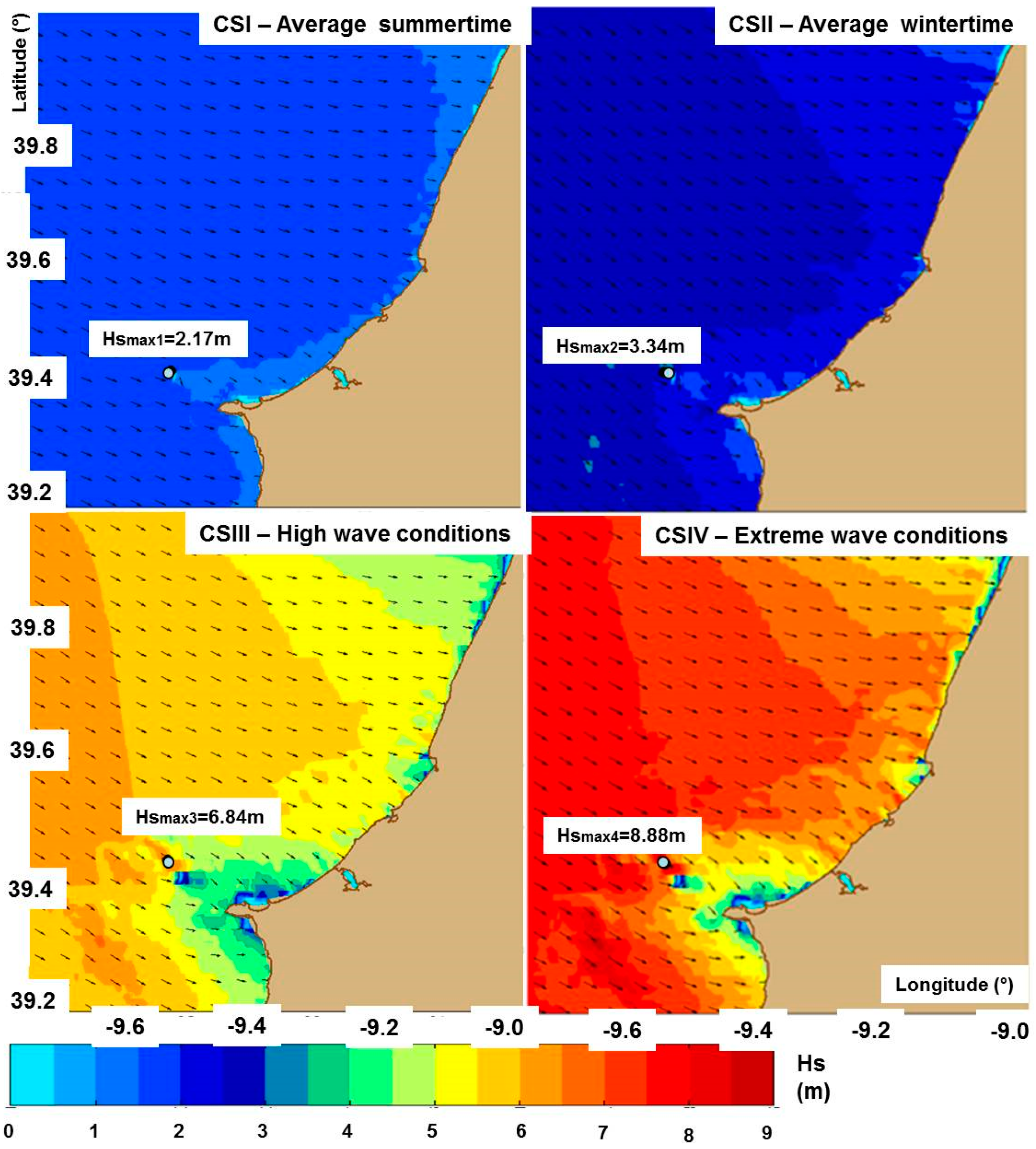
Case Study		Hs (m)		Tp (s)
CSI (total average)		2.0		10.1
CSII (winter average)		2.43		11.0
CSIII (high waves)		4.5		15.0
CSIV (extreme conditions)		8.7		18.0
Mean Wave Direction (°) Nautical Convention		Wind Conditions
		Wind Velocity (m/s)		Wind Direction (°)
Dir1	270	W0 (no wind)	0	-
		W7 (average wind)	7	FW (following wind)	305
				OW (opposite wind)	90
		W22 (high wind)	22	FW (following wind)	305
				OW (opposite wind)	90
Dir2	300	W0 (no wind)	0	-
		W7 (average wind)	7	FW (following wind)	305
				OW (opposite wind)	120
		W22 (high wind)	22	FW (following wind)	305
				OW (opposite wind)	120
Dir3	330	W0 (no wind)	0	-
		W7 (average wind)	7	FW (following wind)	305
				OW (opposite wind)	150
		W22 (high wind)	22	FW (following wind)	305
				OW (opposite wind)	150
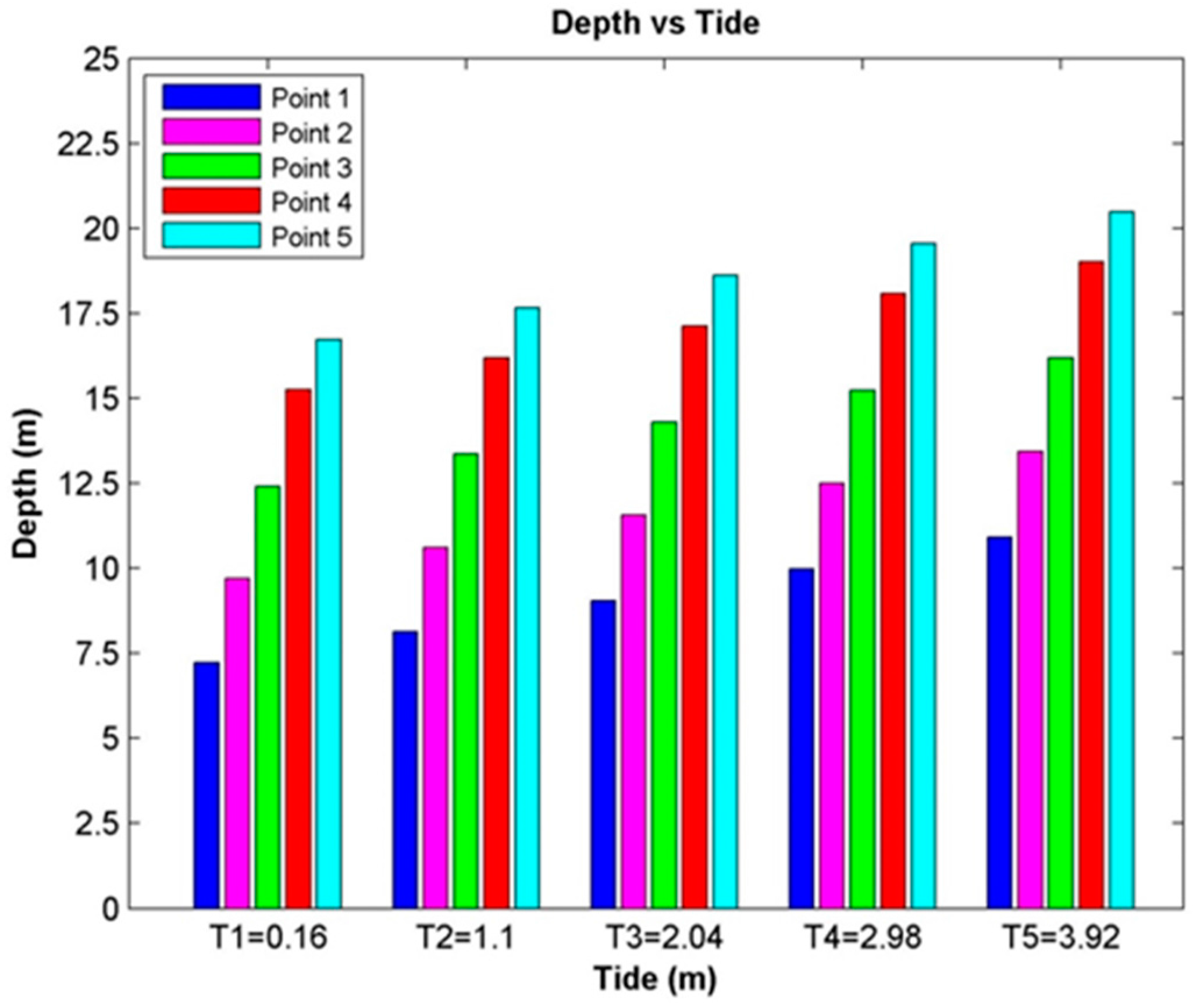
Tide Level	T1	T2	T3	T4	T5
(m)-above the hydrographic zero	0.16	1.1	2.04	2.98	3.92

. At the same time, for these case studies, Figure 5 presents the wave transformation in the third computational level, considering the most frequent direction of the incoming waves, waves coming from the northwest.

3. Study of the Tide and Wind Influences in the High Resolution Computational Domain

A more realistic understanding of the uncertainties in the wave energy resources assessment, especially as regards their variability and predictability, is key to any wave energy project [44,45]. From this perspective, this section will focus on evaluating the influence on the wave conditions of some parameters of the environmental matrix, especially tide and wind. Thus, the main objective of the work is to study in more detail the wave transformation in the coastal area that includes the WaveRoller farm and also to assess in a more accurate way the local effects of the tide and wind on the waves propagating in the vicinity of the wave energy converters. For this, a high-resolution computational domain (denoted as level IV) was also defined and it was connected to the wave prediction system. The geographical space of this high-resolution computational domain is illustrated in Figure 6. Its main characteristics are presented in Table 2, together with those corresponding to the other computational levels.

Five reference points (denoted P1, P2, P3, P4, and P5) have been considered for further analysis and their positions are also illustrated in Figure 6. The point P3 is close to the location of the WaveRoller farm.

The tide conditions were evaluated according to the Tide Tables provided by the Hydrographic Institute of the Portuguese Navy [46] for the years 2012–2014. According to these data, five different levels have been defined, between the low and high tide conditions. They correspond to 0.16 m, 1.1 m, 2.04 m, 2.98 m, and 3.92 m above the hydrographic zero, respectively, and are accounted for in the high-resolution wave model simulations. These five tide levels are presented in Table 3, denoted as T1, T2, T3, T4, and T5. The variation of the water depth due to these five tide levels along the reference points is illustrated in Figure 7. The importance of adding tides into the wave energy study is that they significantly alter the wave’s properties and consequently the local wave power resource [47].

Having as a basis the analysis of the wave conditions presented in Figure 3, three different mean wave directions of the wave propagation on the external boundary of the high-resolution computational domain have been considered for each case study. These are, in nautical terms, Dir1 = 270°, Dir2 = 300°, and Dir3 = 330°. For more efficiency, the position of the wave farm should be perpendicular to the wave direction that contributes with more wave power. Following now the wind conditions presented in Figure 4, three different intensities for the wind speed have been considered. These are denoted as: W0 (no wind situation), W7 (average value for the wind speed, V_w = 7 m/s), and W22 (high value of the wind speed, V_w = 22 m/s). Furthermore, for cases W7 and W22 both directions of following and opposite wind have been taken into account.

Corresponding to this set of simulations, the main wave parameters analysed were significant wave height (H_s) and mean wave direction (Dir) computed by the spectral model using the standard definitions [37]. Additionally, two other wave parameters were also evaluated. The first is the significant wave height of the swell (H_sw), which is the significant wave height associated with the low frequency part of the spectrum, defined as:

$$H_{sw}=4\sqrt{\underset{0}{\overset{{\mathsf{\omega }}_{sw}}{{\displaystyle \int }}}\underset{0}{\overset{2\mathsf{\pi }}{{\displaystyle \int }}}E\left(\mathsf{\omega },\mathsf{\theta }\right)d\mathsf{\omega }d\mathsf{\theta }}$$

(1)

where $E\left(\mathsf{\omega },\mathsf{\theta }\right)$ represents the wave energy spectrum in terms of absolute radian wave frequency (ω), (θ) is the wave direction, and ω_sw = 2πf_sw, the swell frequency (f_sw) was considered here to be 0.1 Hz.

The second is the wave power over one meter of wave front. In SWAN, the wave power components (expressed in W/m, i.e., energy transport per unit length of wave front) are computed with the relationships:

$$\begin{gathered} P_{ x}=\mathsf{\rho }g{{\displaystyle \iint }}^{\text{}}{c}_{x }E\left(\mathsf{\omega },\mathsf{\theta }\right)d\mathsf{\omega }d\mathsf{\theta } \\ {P}_{ y}=\mathsf{\rho }g{{\displaystyle \iint }}^{\text{}}{c}_{y }E\left(\mathsf{\omega },\mathsf{\theta }\right)d\mathsf{\omega }d\mathsf{\theta } \end{gathered}$$

(2)

where x, y are the problem coordinate system (for the spherical coordinates x axis corresponds to the longitude and y axis to the latitude), $\mathsf{\rho }$ is the water density, g is the gravity acceleration, and c_x, c_y are the propagation velocities of the wave energy in the geographical space. The absolute value of the wave power is:

$$P=\sqrt{P_x^2+P_y^2}$$

(3)

The dynamics of the above mentioned wave parameters in relationship with the case studies and all the situations considered (as defined in Table 3) is analysed in the next section.

4. Results and Discussion

The first group of results is presented in Figure 8. This illustrates for all four case studies considered (CS1, CS2, CS3, and CS4) the situations corresponding to the no-wind condition.

This figure presents the variations of the parameters significant wave height (Figure 8a) and significant wave height of the swell (Figure 8b) along the five points (P1, P2, P3, P4, and P5), for the three wave directions (D1 = 270°, D2 = 300°, and D3 = 330°) and the five tide conditions (T1, T2, T3, T4, and T5). The plots show that as the wave direction became more from the north, the wave parameters (H_s and H_sw) for all points of all cases increased, but to a lesser extent for CS1 and CS2, which are the cases for total and winter averages, respectively. With the increase of the tide, the parameters tend to decrease and this becomes more visible in CS3. The differences in these decreases become higher from deep to shallow water. Although the variations of H_s and H_sw are similar, H_sw presents slightly lower values. For all the case studies except CS4, the lowest values of the parameters are encountered at the reference point P5 (which is located in the deepest water), increasing as the water becomes shallower. This feature is best visible for CS3, but it is also characteristic for CS1 and CS2. The explanation of this behaviour is the shoaling process that induces an enhancement of the waves as they propagate from intermediate water depth to shallow water.

The average (7 m/s) and high (22 m/s) wind conditions, resulting from the analysis of Figure 4, considering the situations of following wind, when the wind and the wave directions are almost the same, and of opposite wind, when the wind and wave direction are opposite, were introduced into the model simulations at levels III and IV. The corresponding results for the parameters H_s and H_sw are presented in Figure 9, Figure 10, Figure 11 and Figure 12, following the same representation as in Figure 8.

In each of these figures, subplot (a) is related to the situation of the following wind while subplot (b) is related to the situation of the opposite wind. In Figure 9 (H_s in average wind), the general tendencies are rather similar to those presented in Figure 8. We can observe, however, that in the case of the following wind (Figure 9a), the significant wave heights are higher than in the case of the opposite wind (Figure 9b). The same trend is also noticeable in Figure 10 (H_sw in average wind).

Although the general trends of Figure 11 and Figure 12 (high wind) are in some sense similar to the corresponding ones in Figure 9 and Figure 10 (average wind), there are some particularities that can be better noticed in high-wind situations. In terms of significant wave heights, in the situation of the following wind, this implies an enhancement of more than 2 m for CS1 and CS2; this enhancement decreases to about 1.5 m and 1 m in CS3 and CS4, respectively.

In the case of the opposite wind, some interesting results can be noticed in relationship with CS1 and CS2 when an enhancement of about 0.5 m (or more) occurs. On the other hand, for CS3 and CS4 there are no notable differences in comparison with the average wind situation. As regards H_sw, the general tendencies are similar to those related to H_s. In the situation of the following wind this implies now an enhancement of about 1.5 m for CS1, CS2, and CS3 and this enhancement decreases to less than 1 m in CS4. Nevertheless, in the case of the opposite wind an enhancement of about 0.5 m (or more) occurs again in CS1 and CS2, but only for the direction D1. For the other two directions considered (D2 and D3), there is no enhancement of this parameter, and moreover even a small decay appears. In order to better assess the variation range of the main wave parameters, the numerical results corresponding to the reference points of the WaveRoller device and seaward (P3, P4, and P5) and to the extreme values of the tide level (T1 and T5) are presented separately for each case study in

Table 4. SWAN results for CS1, corresponding to the reference points P3, P4, and P5, the tide levels T1 and T5, and the wind conditions W0, W7, and W22, in terms of the wave parameters H_s, H_sw, and P_w.

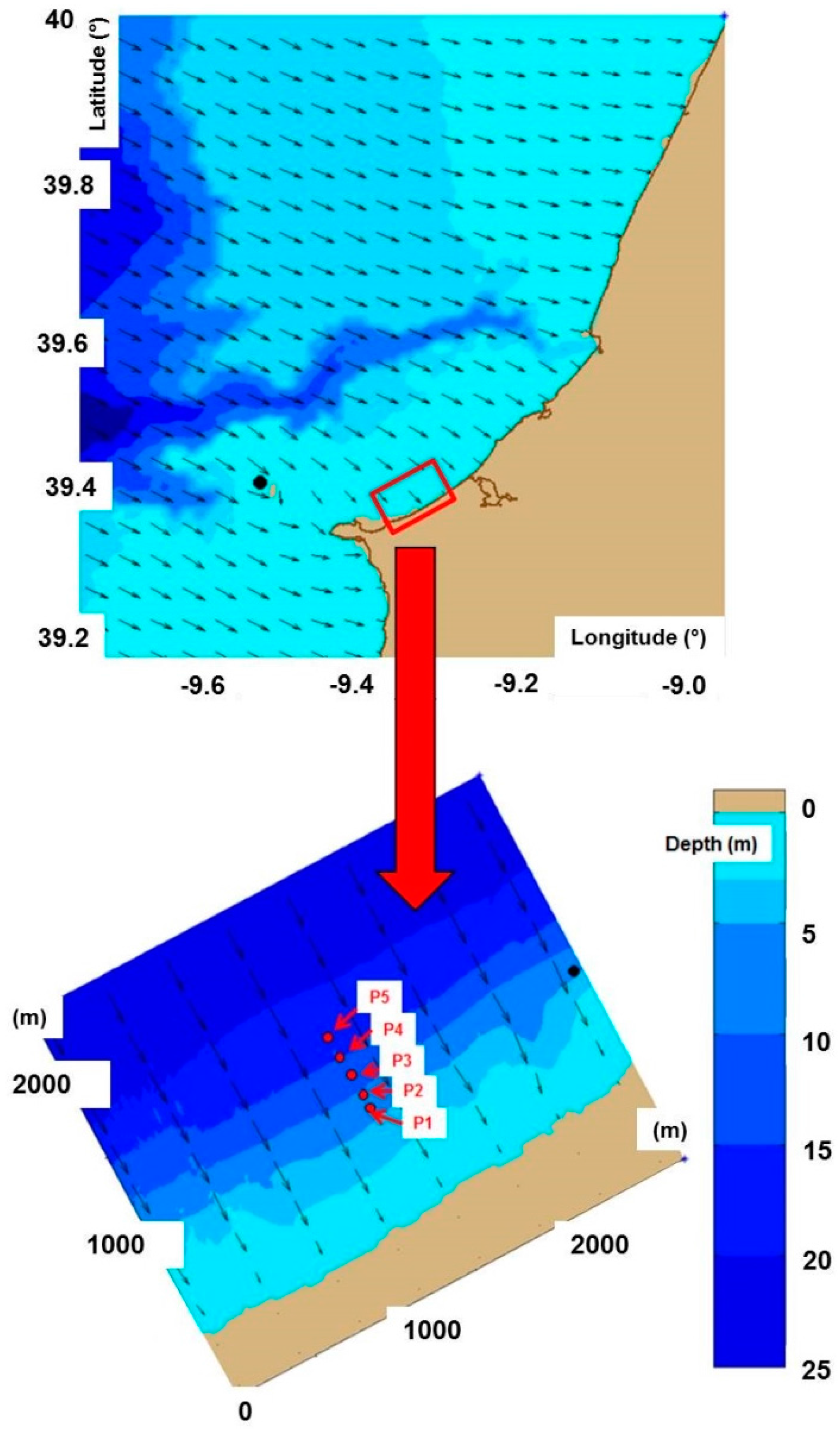
CS1			P3			P4			P5
			Hs	Hsw	Pw	Hs	Hsw	Pw	Hs	Hsw	Pw
			m	m	kW/m	m	m	kW/m	m	m	kW/m
D1	W0	T1	1.07	0.67	5.16	1.08	0.66	5.26	1.06	0.64	5.06
		T5	1.06	0.65	5.15	1.07	0.65	5.22	1.06	0.64	5.07
	W7-FW	T1	1.25	0.77	6.91	1.26	0.77	7.03	1.24	0.75	6.76
		T5	1.24	0.75	6.90	1.25	0.75	6.98	1.24	0.74	6.78
	W7-OW	T1	1.09	0.67	5.19	1.09	0.66	5.27	1.07	0.65	5.06
		T5	1.07	0.65	5.17	1.08	0.65	5.23	1.07	0.64	5.08
	W22-FW	T1	3.68	2.21	57.89	3.68	2.19	58.44	3.62	2.13	55.91
		T5	3.64	2.15	57.70	3.66	2.15	57.98	3.62	2.11	56.07
	W22-OW	T1	1.78	0.97	12.01	1.83	0.99	12.90	1.84	1.00	13.10
		T5	1.80	0.97	12.44	1.84	0.99	13.17	1.85	1.00	13.35
D2	W0	T1	1.35	0.84	8.21	1.36	0.83	8.32	1.33	0.81	7.97
		T5	1.34	0.82	8.19	1.35	0.82	8.25	1.33	0.81	8.00
	W7-FW	T1	1.51	0.93	10.11	1.52	0.93	10.24	1.49	0.90	9.81
		T5	1.49	0.91	10.08	1.51	0.91	10.16	1.49	0.89	9.85
	W7-OW	T1	1.36	0.84	8.21	1.37	0.83	8.31	1.34	0.81	7.96
		T5	1.35	0.82	8.18	1.36	0.82	8.25	1.34	0.81	7.99
	W22-FW	T1	3.89	2.34	65.04	3.89	2.32	65.66	3.82	2.26	62.75
		T5	3.85	2.29	64.79	3.87	2.28	65.05	3.82	2.24	62.87
	W22-OW	T1	1.47	0.80	7.28	1.48	0.79	7.38	1.47	0.77	7.08
		T5	1.45	0.78	7.28	1.47	0.78	7.34	1.46	0.77	7.12
D3	W0	T1	1.47	0.91	9.71	1.48	0.91	9.82	1.45	0.88	9.40
		T5	1.45	0.89	9.68	1.47	0.89	9.74	1.45	0.88	9.43
	W7-FW	T1	1.63	1.01	11.78	1.64	1.00	11.90	1.61	0.97	11.39
		T5	1.61	0.98	11.74	1.62	0.98	11.81	1.61	0.96	11.44
	W7-OW	T1	1.48	0.91	9.70	1.49	0.91	9.81	1.46	0.88	9.39
		T5	1.46	0.89	9.67	1.47	0.89	9.74	1.46	0.88	9.43
	W22-FW	T1	3.96	2.39	67.65	3.97	2.37	68.25	3.90	2.31	65.21
		T5	3.92	2.33	67.40	3.94	2.33	67.62	3.89	2.29	65.35
	W22-OW	T1	1.51	0.83	7.66	1.53	0.83	7.74	1.52	0.80	7.37
		T5	1.49	0.81	7.64	1.52	0.81	7.68	1.52	0.80	7.41

,

Table 5. SWAN results for CS2, corresponding to the reference points P3, P4, and P5, the tide levels T1 and T5, and the wind conditions W0, W7, and W22, in terms of the wave parameters H_s, H_sw, and P_w.

CS2			P3			P4			P5
			Hs	Hsw	Pw	Hs	Hsw	Pw	Hs	Hsw	Pw
			m	m	kW/m	m	m	kW/m	m	m	kW/m
D1	W0	T1	1.28	1.00	7.77	1.28	0.99	7.91	1.25	0.96	7.57
		T5	1.26	0.97	7.80	1.27	0.98	7.90	1.25	0.96	7.65
	W7-FW	T1	1.46	1.13	9.97	1.46	1.12	10.15	1.43	1.09	9.72
		T5	1.44	1.10	10.01	1.45	1.10	10.13	1.43	1.08	9.81
	W7-OW	T1	1.32	1.02	8.16	1.32	1.02	8.29	1.30	0.99	7.93
		T5	1.30	1.00	8.19	1.31	1.00	8.28	1.29	0.98	8.01
	W22-FW	T1	3.82	2.30	62.75	3.83	2.28	63.41	3.76	2.22	60.64
		T5	3.78	2.24	62.51	3.80	2.24	62.82	3.76	2.20	60.75
	W22-OW	T1	2.00	1.42	16.48	2.03	1.43	17.35	2.03	1.42	17.30
		T5	2.00	1.40	16.90	2.03	1.42	17.65	2.03	1.42	17.65
D2	W0	T1	1.67	1.30	13.13	1.66	1.29	13.30	1.63	1.25	12.70
		T5	1.64	1.27	13.17	1.65	1.27	13.28	1.62	1.24	12.83
	W7-FW	T1	1.80	1.39	15.10	1.79	1.38	15.30	1.76	1.34	14.61
		T5	1.77	1.36	15.15	1.78	1.36	15.27	1.75	1.33	14.75
	W7-OW	T1	1.67	1.30	13.13	1.67	1.29	13.29	1.64	1.25	12.69
		T5	1.63	1.27	13.17	1.65	1.27	13.27	1.63	1.24	12.82
	W22-FW	T1	4.15	3.15	78.44	4.14	3.12	79.26	4.05	3.03	75.53
		T5	4.09	3.07	78.65	4.09	3.06	78.99	4.03	3.00	76.15
	W22-OW	T1	1.73	1.23	11.70	1.74	1.22	11.79	1.73	1.19	11.22
		T5	1.71	1.21	11.72	1.72	1.20	11.78	1.71	1.18	11.35
D3	W0	T1	1.83	1.42	15.77	1.82	1.41	15.95	1.78	1.37	15.22
		T5	1.80	1.39	15.82	1.81	1.39	15.93	1.78	1.36	15.38
	W7-FW	T1	1.95	1.51	17.74	1.94	1.49	17.94	1.90	1.45	17.12
		T5	1.92	1.47	17.80	1.92	1.47	17.92	1.90	1.44	17.30
	W7-OW	T1	1.83	1.42	15.76	1.83	1.41	15.94	1.79	1.37	15.20
		T5	1.80	1.39	15.82	1.81	1.39	15.92	1.79	1.36	15.37
	W22-FW	T1	4.24	3.23	82.18	4.23	3.19	83.02	4.14	3.10	79.09
		T5	4.18	3.15	82.45	4.19	3.14	82.76	4.13	3.08	79.76
	W22-OW	T1	1.83	1.32	13.25	1.84	1.31	13.38	1.82	1.27	12.72
		T5	1.80	1.29	13.29	1.82	1.29	13.36	1.81	1.26	12.85

,

Table 6. SWAN results for CS3, corresponding to the reference points P3, P4, and P5, the tide levels T1 and T5, and the wind conditions W0, W7, and W22, in terms of the wave parameters H_s, H_sw, and P_w.

CS3			P3			P4			P5
			Hs	Hsw	Pw	Hs	Hsw	Pw	Hs	Hsw	Pw
			m	m	kW/m	m	m	kW/m	m	m	kW/m
D1	W0	T1	2.44	2.31	32.75	2.41	2.27	33.29	2.33	2.19	31.57
		T5	2.39	2.25	33.69	2.37	2.23	34.09	2.32	2.17	32.70
	W7-FW	T1	2.53	2.38	34.75	2.49	2.34	35.33	2.41	2.26	33.51
		T5	2.47	2.32	35.75	2.45	2.30	36.17	2.39	2.24	34.70
	W7-OW	T1	2.47	2.33	33.33	2.44	2.29	33.87	2.36	2.21	32.11
		T5	2.42	2.27	34.29	2.40	2.25	34.68	2.34	2.19	33.26
	W22-FW	T1	4.54	4.21	109.68	4.48	4.14	111.41	4.33	3.99	105.34
		T5	4.44	4.10	112.73	4.40	4.06	113.60	4.29	3.95	108.73
	W22-OW	T1	3.01	2.75	46.59	2.97	2.70	47.22	2.89	2.62	44.76
		T5	2.96	2.69	47.96	2.93	2.66	48.35	2.87	2.59	46.38
D2	W0	T1	3.14	2.97	54.08	3.10	2.92	54.76	3.00	2.81	51.82
		T5	3.07	2.90	55.63	3.05	2.86	56.09	2.98	2.79	53.70
	W7-FW	T1	3.19	3.01	55.54	3.14	2.95	56.25	3.04	2.85	53.23
		T5	3.12	2.93	57.13	3.09	2.90	57.61	3.02	2.83	55.15
	W7-OW	T1	3.19	3.01	55.52	3.14	2.95	56.22	3.04	2.85	53.20
		T5	3.12	2.93	57.11	3.09	2.90	57.58	3.02	2.83	55.13
	W22-FW	T1	5.06	4.61	133.41	5.03	4.56	136.70	4.88	4.40	129.46
		T5	4.99	4.52	138.28	4.95	4.48	139.18	4.84	4.37	133.25
	W22-OW	T1	3.24	2.99	54.63	3.20	2.93	55.21	3.10	2.83	52.16
		T5	3.18	2.91	56.14	3.16	2.88	56.52	3.09	2.81	54.04
D3	W0	T1	3.55	3.36	69.04	3.50	3.29	69.91	3.39	3.18	66.08
		T5	3.47	3.27	70.98	3.44	3.23	71.49	3.36	3.15	68.42
	W7-FW	T1	3.60	3.40	70.71	3.55	3.33	71.59	3.43	3.22	67.67
		T5	3.52	3.31	72.69	3.49	3.27	73.21	3.41	3.19	70.06
	W7-OW	T1	3.56	3.36	69.03	3.50	3.29	69.89	3.39	3.18	66.06
		T5	3.48	3.27	70.96	3.45	3.23	71.47	3.37	3.15	68.40
	W22-FW	T1	5.27	4.81	145.20	5.27	4.78	150.01	5.11	4.62	142.18
		T5	5.23	4.74	152.12	5.19	4.70	153.03	5.08	4.58	146.51
	W22-OW	T1	3.57	3.31	66.78	3.53	3.25	67.54	3.43	3.13	63.75
		T5	3.49	3.22	68.62	3.47	3.19	69.07	3.39	3.10	66.03

and

Table 7. SWAN results for CS4, corresponding to the reference points P3, P4, and P5, the tide levels T1 and T5, and the wind conditions W0, W7, and W22, in terms of the wave parameters H_s, H_sw, and P_w.

CS3			P3			P4			P5
			Hs	Hsw	Pw	Hs	Hsw	Pw	Hs	Hsw	Pw
			m	m	kW/m	m	m	kW/m	m	m	kW/m
D1	W0	T1	4.07	3.94	94.21	4.01	3.87	95.84	3.86	3.72	90.59
		T5	3.97	3.84	97.64	3.93	3.80	98.71	3.83	3.69	94.45
	W7-FW	T1	4.08	3.94	94.23	4.01	3.87	95.86	3.87	3.72	90.61
		T5	3.98	3.84	97.66	3.94	3.80	98.73	3.84	3.69	94.46
	W7-OW	T1	4.07	3.93	93.79	4.00	3.86	95.38	3.86	3.72	90.14
		T5	3.97	3.83	97.20	3.93	3.79	98.24	3.83	3.68	93.98
	W22-FW	T1	5.30	5.07	156.25	5.27	5.03	162.48	5.09	4.84	153.65
		T5	5.24	5.00	166.23	5.18	4.94	167.84	5.04	4.80	160.26
	W22-OW	T1	4.27	4.08	100.59	4.20	3.99	102.07	4.06	3.85	96.26
		T5	4.18	3.97	104.26	4.13	3.92	105.08	4.03	3.81	100.34
D2	W0	T1	5.06	4.90	145.29	5.00	4.83	149.32	4.83	4.65	140.98
		T5	4.98	4.81	152.91	4.92	4.75	154.30	4.79	4.61	147.30
	W7-FW	T1	5.05	4.88	144.25	4.99	4.81	148.18	4.81	4.64	139.90
		T5	4.96	4.79	151.76	4.91	4.73	153.13	4.78	4.60	146.17
	W7-OW	T1	5.06	4.90	144.76	5.00	4.82	148.73	4.82	4.65	140.42
		T5	5.00	4.80	152.33	4.92	4.74	153.70	4.79	4.61	146.72
	W22-FW	T1	5.80	5.57	188.31	5.88	5.62	202.92	5.70	5.44	193.22
		T5	5.88	5.63	209.82	5.82	5.56	212.07	5.66	5.40	202.40
	W22-OW	T1	5.07	4.87	143.18	5.02	4.80	147.30	4.86	4.63	139.02
		T5	5.00	4.78	150.93	4.95	4.72	152.22	4.82	4.59	145.24
D3	W0	T1	5.51	5.34	172.14	5.50	5.32	180.55	5.32	5.13	170.96
		T5	5.49	5.30	185.7	5.43	5.24	187.44	5.29	5.09	178.93
	W7-FW	T1	5.51	5.33	171.81	5.50	5.31	180.28	5.32	5.13	170.79
		T5	5.49	5.30	185.67	5.43	5.24	187.41	5.29	5.09	178.91
	W7-OW	T1	5.52	5.35	172.72	5.52	5.33	181.39	5.34	5.14	171.88
		T5	5.51	5.32	186.87	5.45	5.25	188.63	5.31	5.11	180.08
	W22-FW	T1	5.92	5.70	196.67	6.04	5.79	214.67	5.87	5.61	205.16
		T5	6.07	5.81	223.35	6.01	5.74	226.15	5.85	5.58	215.77
	W22-OW	T1	5.50	5.30	169.33	5.51	5.28	178.00	5.34	5.10	168.61
		T5	5.50	5.28	183.41	5.45	5.21	185.08	5.31	5.06	176.60

, respectively. The values show what was mentioned before, that with the wave direction coming more from the north (330°), there is an increase of the wave parameters Hs and Hsw. In the case of tidal variations, the values decrease as this parameter increases. For CS1 and CS2 the differences between these points (P3, P4, and P5) are insignificant, but increase from CS3 to CS4, with P3 having the highest values and P5 the lowest.

Another wave parameter that will be analysed, also presented in the previous tables, is the wave power over one meter of wave front (P_w). Figure 13, Figure 14 and Figure 15 illustrate the variation of this parameter along the five reference points, for the three wave directions previously considered (D1 = 270°, D2 = 300°, and D3 = 330°) and for the five different tide levels, just like in the preceding figures.

Comparing the variations of the wave power presented in Figure 13, Figure 14 and Figure 15, with the variations of the parameters H_s and H_sw presented in Figure 8, Figure 9, Figure 10, Figure 11 and Figure 12, it can be seen that P_w is a very sensitive parameter to both wind and tide conditions. At this point, it can be also highlighted that the variations of the wave power presented in Figure 13, Figure 14 and Figure 15 give a quantitative representation of the way how this parameter is changed under various wave conditions and tide levels. These can be used to directly estimate the wave power in the target area for various conditions and also compared with similar results obtained in other coastal environments where wave energy farms are operating, or are going to be implemented.

In relationship to the variation of the mean wave direction, the same trend as in the case of the previous parameters analysed (H_s and H_sw) is observed. However, this time the differences are relatively more significant. Thus, P_w increases as the incoming wave direction on the external boundary is increased from 270° to 330°. In the case of the wind, until we get to the average speed values for both the following and opposite wind directions, the influence is not really visible. As for tides, the variation of P_w is much more visible than H_s and H_sw in the shallowest points (P1 and P2).

Taking into account the analysis of the mean wave direction in the target area presented in Figure 3, the most frequent wave conditions correspond to mean wave directions between D2 and D3. From this perspective, the results corresponding to these two directions should be considered statistically more relevant. Corresponding to the wave directions between D2 and D3, the wave power for the average wind has values in the ranges 10–20 kW/m for CS1 and CS2 and 50–70 kW/m for CS3. As regards CS4, which is the most energetic case, the range is considerably wider, 100–180 kW/m.

For the high wind conditions, while the opposite wind does not much influence the Pw variation, the following wind leads to an enhancement of this parameter between the directions D2 and D3 to values in the ranges 50–80 kW/m for CS1 and CS2 and 90–140 kW/m for CS3. For CS4, the range of the wave power now becomes 110–220 kW/m. Finally, it has to be highlighted that in this situation of high wind conditions, the tide level influenced all the cases, CS4 in a strong way and CS2 and CS1less so.

5. Conclusions

The present work presents a study on the influence of the local tide and wind on the wave conditions at the Portuguese nearshore, close to the city of Peniche. For this purpose, a wave prediction system, based on the spectral phase averaged model SWAN, was focused on the target area in a multi-level modelling scheme. This included four computational levels, corresponding to the entire west Iberian nearshore (Level I), the central part of the Portuguese nearshore (Level II), the vicinity of Cape Peniche (Level III), and finally a high-resolution computational domain centred on the site where the WaveRoller devices operate (Level IV), respectively. In these new set of simulations, the tide effect has been also accounted for.

The results show that P_w is the most sensitive parameter when comparing with H_s and H_sw. For the same H_s of the incoming waves, the highest sensitivity occurs in relationship with the wave direction. Thus, the expected wave power is lower when the wave direction is from the west and increases gradually, but in a substantial way, as the direction of the incoming waves moves to the north. As regards the tide, its influence becomes visible mostly for the high waves (when the process of wave breaking starts earlier). This especially concerns reference points P1 and P2, which are located in shallower water (between 7.5 m and 14 m, as a function of the tide conditions). While the average wind conditions (7–8 m/s) do not significantly influence the distribution of the wave power, the high-intensity following wind leads to a visible enhancement of the wave power, but also to a higher sensitivity of this parameter to the tide variations.

References

- European Renewable Energy Council (EREC). Mapping Renewable Energy Pathways towards 2020; EU Roadmap: Brussels, Belgium, 2011. [Google Scholar]
- The European Marine Energy Centre (EMEC). Assessment of Wave Energy Resource; The European Marine Energy Centre Ltd.: London, UK, 2009; p. 36. [Google Scholar]
- Clement, A.; McCullen, P.; Falcao, A.; Fiorentino, A.; Gardner, F.; Hammarlund, K.; Lemonis, G.; Lewis, T.; Nielsen, K.; Petroncini, S.; et al. Wave energy in Europe: Current status and perspectives. Renew. Sustain. Energy Rev. 2002, 6, 405–431. [Google Scholar] [CrossRef]
- Silva, D.; Bento, A.R.; Martinho, P.; Guedes Soares, C. High resolution local wave energy modelling for the Iberian Peninsula. Energy 2015, 91, 1099–1112. [Google Scholar] [CrossRef]
- Rusu, E.; Guedes Soares, C. Wave energy assessments in the coastal environment of Portugal continental. In Proceedings of the 27th International Conference on Offshore Mechanics and Arctic Engineering—OMAE 2008, Estoril, Portugal, 15–20 June 2008; Volume 6, pp. 761–772.
- Dalton, G.J.; Alcorn, R.; Lewis, T. Case study feasibility analysis of the Pelamis wave energy convertor in Ireland, Portugal and North America. Renew. Energy 2010, 35, 443–455. [Google Scholar] [CrossRef]
- Cunha, P.P.; Gouveia, M.P. The Nazaré Coast, the Submarine Canyon and the Giant Waves: A Synthesis; Marine and Environmental Sciences Centre: Coimbra, Portugal, 2015; p. 32. [Google Scholar]
- Sebastião, P.; Guedes Soares, C.; Alvarez, E. 44 Years Hindcast of Sea Level in the Atlantic Coast of Europe. Coast. Eng. 2008, 55, 843–848. [Google Scholar] [CrossRef]
- Sauvaget, P.; David, E.; Guedes Soares, C. Modelling Tidal Currents on the Coast of Portugal. Coast. Eng. 2000, 40, 393–409. [Google Scholar] [CrossRef]
- Almeida, M.M.; Guedes Soares, C. Numerical investigation of the tidal energy potential in the Portuguese continental shelf. In Renewable Energies Offshore; Guedes Soares, C., Ed.; Taylor & Francis Group: London, UK, 2015; pp. 177–182. [Google Scholar]
- WaveRoller Concept. Available online: http://aw-energy.com/about-waveroller/waveroller-concept (accessed on 4 December 2015).
- AM Energy & LENA Group. 1 MW Wave Energy Power Plant Peniche—Portugal, Waveroller Technology. 2007. Available online: http://www.cm-peniche.pt/_uploads/pdf_noticias/waverollerawenergyoyeneolicasagrupolena.pdf (accessed on 4 December 2015).
- Rusu, E.; Guedes Soares, C. Numerical modeling to estimate the spatial distribution of the wave energy in the Portuguese nearshore. Renew. Energy 2009, 34, 1501–1516. [Google Scholar] [CrossRef]
- Lucas, J.; Livinstone, M.; Vuorinen, M.; Cruz, J. Development of a wave energy converter (WEC) design tool—Application to the WaveRoller WEC including validation of numerical estimates. In Proceedings of the ICOE 2012, Dublin, Ireland, 17–19 October 2012.
- The Wamdi Group. The WAM model—A third generation ocean wave prediction model. J. Phys. Oceanogr. 1988, 18, 1775–1810. [Google Scholar]
- Booij, N.; Ris, R.C.; Holthuijsen, L.H. A third-generation wave model for coastal regions. I—Model description and validation. J. Geophys. Res. 1999, 104, 7649–7666. [Google Scholar] [CrossRef]
- Rusu, L.; Pilar, P.; Guedes Soares, C. Reanalysis of the wave conditions in the approaches to the Portuguese port of Sines. In Maritime Transportation and Exploitation of Ocean and Coastal Resources; Guedes Soares, C., Garbatov, Y., Fonseca, N., Eds.; Taylor & Francis Group: London, UK, 2005; pp. 1137–1142. [Google Scholar]
- Rusu, L.; Pilar, P.; Guedes Soares, C. Hindcast of the wave conditions along the west Iberian coast. Coast. Eng. 2008, 55, 906–919. [Google Scholar] [CrossRef]
- Rusu, L.; Guedes Soares, C. Evaluation of a high-resolution wave forecasting system for the approaches to ports. Ocean Eng. 2013, 58, 224–238. [Google Scholar] [CrossRef]
- Rusu, E.; Guedes Soares, C. Wave modeling at the entrance of ports. Ocean Eng. 2011, 38, 2089–2109. [Google Scholar] [CrossRef]
- Gonçalves, M.; Rusu, E.; Guedes Soares, C. Evaluation of Two Spectral Wave Models in Coastal Areas. J. Coast. Res. 2015, 31, 326–339. [Google Scholar] [CrossRef]
- Rusu, E.; Gonçalves, M.; Guedes Soares, C. Evaluation of the wave transformation in an open bay with two spectral models. Ocean Eng. 2011, 38, 1763–1781. [Google Scholar] [CrossRef]
- Rusu, L.; Bernardino, M.; Guedes Soares, C. Modelling the influence of currents on wave propagation at the entrance of the Tagus estuary. Ocean Eng. 2011, 38, 1174–1183. [Google Scholar] [CrossRef]
- Guedes Soares, C.; Rusu, L.; Bernardino, M.; Pilar, P. An operational wave forecasting system for the Portuguese continental coastal area. J. Oper. Oceanogr. 2011, 4, 16–26. [Google Scholar] [CrossRef]
- Rusu, L.; Guedes Soares, C. Local data assimilation scheme for wave predictions close to the Portuguese ports. J. Oper. Oceanogr. 2014, 7, 45–57. [Google Scholar] [CrossRef]
- Almeida, S.; Rusu, L.; Guedes Soares, C. Application of the Ensemble Kalman Filter to a high-resolution wave forecasting model for wave height forecast in coastal areas. In Maritime Technology and Engineering; Guedes Soares, C., Santos, T.A., Eds.; Taylor & Francis Group: London, UK, 2015; pp. 1349–1354. [Google Scholar]
- Rusu, L.; Guedes Soares, C. Impact of assimilating altimeter data on wave predictions in the western Iberian coast. Ocean Model. 2015, 96, 126–135. [Google Scholar] [CrossRef]
- Rusu, E.; Guedes Soares, C. Wave energy pattern around the Madeira Islands. Energy 2012, 45, 771–785. [Google Scholar] [CrossRef]
- Rusu, L.; Guedes Soares, C. Wave energy assessments in the Azores islands. Renew. Energy 2012, 45, 183–196. [Google Scholar] [CrossRef]
- Tolman, H.L. A third-generation model for wind waves on slowly varying, unsteady and inhomogeneous depths and currents. J. Phys. Oceanogr. 1991, 21, 782–797. [Google Scholar] [CrossRef]
- Silva, D.; Martinho, P.; Guedes Soares, C. Modeling wave energy for the Portuguese coast. In Maritime Engineering and Technology; Guedes, S.C., Garbatov, Y., Sutulo, S., Santos, T.A., Eds.; Taylor & Francis Group: London, UK, 2012; pp. 647–653. [Google Scholar]
- Silva, D.; Rusu, E.; Guedes Soares, C. Evaluation of various technologies for wave energy conversion in the Portuguese nearshore. Energies 2013, 6, 1344–1364. [Google Scholar] [CrossRef]
- Guedes Soares, C.; Bento, A.R.; Goncalves, M.; Silva, D.; Martinho, P. Numerical evaluation of the wave energy resource along the Atlantic European coast. Comput. Geosci. 2014, 71, 37–49. [Google Scholar] [CrossRef]
- Goncalves, M.; Martinho, P.; Guedes Soares, C. Wave energy conditions in the western French coast. Renew. Energy 2014, 62, 155–163. [Google Scholar] [CrossRef]
- Goncalves, M.; Martinho, P.; Guedes Soares, C. Assessment of wave energy in the Canary Islands. Renew. Energy 2014, 68, 774–784. [Google Scholar] [CrossRef]
- Bento, A.R.; Martinho, P.; Guedes Soares, C. Numerical modelling of the wave energy in Galway Bay. Renew. Energy 2015, 78, 457–466. [Google Scholar] [CrossRef]
- SWAN Team. Scientific and Technical Documentation, SWAN Cycle III Version 41.01; Delft University of Technology, Department of Civil Engineering: Delft, The Netherlands, 2015. [Google Scholar]
- Wang, W.; Barker, D.; Bray, J.; Bruyère, C.; Duda, M.; Dudhia, J.; Gill, D.; Michalakes, J. User’s Guide for Advanced Research WRF (ARW) Modeling System Version 3; Mesoscale and Microscale Meteorology Division—National Center for Atmospheric Research (MMM-NCAR): Boulder, CO, USA, 2007. [Google Scholar]
- Salvacao, N.; Bernardino, M.; Guedes Soares, C. Assessing mesoscale wind simulations in different environments. Comput. Geosci. 2014, 71, 28–36. [Google Scholar] [CrossRef]
- Salvacao, N.; Bernardino, M.; Guedes Soares, C. Assessing the offshore wind energy potential along coasts of Portugal and Galicia. In Developments in Maritime Transportation and Exploitation of Sea Resources; Guedes Soares, C., Lopez Pena, F., Eds.; Taylor & Francis Group: London, UK, 2014; pp. 995–1002. [Google Scholar]
- Rusu, E.; Rusu, L.; Guedes Soares, C. Prediction of extreme wave conditions in the Black sea with numerical models. In Proceedings of the 9th International Workshop on Wave Hindcasting and Forecasting (9WW), Victoria, BC, Canada, 24–29 September 2006.
- Rusu, E.; Guedes Soares, C. Validation of two wave and nearshore current models. J. Waterw. Port Coast. Ocean Eng. 2010, 136, 27–45. [Google Scholar] [CrossRef]
- Conley, D.C.; Rusu, E. Tests of Wave Shoaling and Surf Models in a Partially Enclosed Basin, Maritime Transportation and Exploitation of Ocean and Coastal Resources; Taylor & Francis Publications: London, UK, 2006; Volume 2, pp. 1015–1021. [Google Scholar]
- Mackay, E.B.L.; Bahaj, A.S.; Challenor, P.G. Uncertainty in wave energy resource assessment. Part 1: Historic data. Renew. Energy 2010, 35, 1792–1808. [Google Scholar] [CrossRef]
- Mackay, E.B.L.; Bahaj, A.S.; Challenor, P.G. Uncertainty in wave energy resource assessment. Part 2: Variability and predictability. Renew. Energy 2010, 35, 1809–1819. [Google Scholar] [CrossRef]
- Instituto Hidrografico, Tide Tables 2012–2014. Available online: http://www.hidrografico.pt/download-tabelas-mare.php (accessed on 9 June 2015).
- Hashemi, M.R.; Neill, S.P. The role of tides in shelf-scale simulations of the wave energy resource. Renew. Energy 2014, 69, 300–310. [Google Scholar] [CrossRef]