
Analytical Modeling of Wind Farms: A New Approach for Power Prediction


1
Wind Engineering and Renewable Energy Laboratory (WIRE), École Polytechnique Fédérale de Lausanne (EPFL), EPFL-ENAC-IIE-WIRE, 1015 Lausanne, Switzerland
2
Stream Biofilm and Ecosystem Research Laboratory (SBER), École Polytechnique Fédérale de Lausanne (EPFL), EPFL-ENAC-IIE-SBER, 1015 Lausanne, Switzerland
*
Author to whom correspondence should be addressed.
Energies 2016, 9(9), 741; https://doi.org/10.3390/en9090741
Submission received: 11 April 2016
/
Revised: 18 August 2016
/
Accepted: 31 August 2016
/
Published: 15 September 2016
Abstract
:Wind farm power production is known to be strongly affected by turbine wake effects. The purpose of this study is to develop and test a new analytical model for the prediction of wind turbine wakes and the associated power losses in wind farms. The new model is an extension of the one recently proposed by Bastankhah and Porté-Agel for the wake of stand-alone wind turbines. It satisfies the conservation of mass and momentum and assumes a self-similar Gaussian shape of the velocity deficit. The local wake growth rate is estimated based on the local streamwise turbulence intensity. Superposition of velocity deficits is used to model the interaction of the multiple wakes. Furthermore, the power production from the wind turbines is calculated using the power curve. The performance of the new analytical wind farm model is validated against power measurements and large-eddy simulation (LES) data from the Horns Rev wind farm for a wide range of wind directions, corresponding to a variety of full-wake and partial-wake conditions. A reasonable agreement is found between the proposed analytical model, LES data, and power measurements. Compared with a commonly used wind farm wake model, the new model shows a significant improvement in the prediction of wind farm power.
1. Introduction
Renewable energies play an increasingly important role in the global energy market as sources of sustainable and clean energy. Specifically, wind energy is witnessing continuous growth at an average annual rate of approximately 25% and currently contributes to more than 2.6% of electricity generation worldwide. This contribution is expected to increase to 18% of the world’s electricity generation by 2050 [1].
Power production from wind farms is significantly affected by wind turbine wakes. This power loss can be up to 25% of the total power output [2]. For this reason, the accurate prediction of turbine wakes is imperative to minimize power losses and, thus, increase the overall efficiency of wind farms. Turbine wake effects have been investigated in numerous experimental, numerical, and analytical studies. Recent advances in turbulence-resolving computational fluid dynamics methods, such as large-eddy simulation (LES) and cutting-edge experimental techniques, have allowed detailed characterization of wind turbine wake flows. Although both experimental and numerical approaches have the potential of providing accurate results, the simplicity and low computational cost associated with analytical models make them appealing for wind farm optimization purposes [3,4]. For that reason, analytical modeling of wind farms has been and continues to be an important topic of research in the field of wind energy. Analytical wind farm models can be divided into two main types: Kinematic models (e.g., [5,6]) and distributed roughness models (e.g., [7,8,9]). Kinematic models consider each turbine wake individually and apply superposition principles to address the interaction of neighboring wakes. In distributed roughness models, turbines act as distributed roughness elements in which the ambient atmospheric flow is modified. Furthermore, there are some models that combine kinematic models with distributed roughness models (e.g., [10,11]). In the present study, we propose a new wind farm analytical model, which is a type of kinematic model, to predict the performance of wind farms of arbitrary size and layout. Although several analytical wind farm models have been developed to estimate the power generated from wind turbines, there are still some critical issues related to the modeling of the velocity deficit and the velocity deficit superposition (due to the interaction of multiple wakes) that need to be addressed to increase the accuracy and robustness of these models.
Several analytical wake models have been developed to estimate the wake flow inside wind farms [5,12,13,14,15]. One of the most commonly used wake models is the one proposed by Jensen [6,12]. This model, which has been extensively used in the literature (e.g., [16]) and in commercial software (e.g., [17,18,19,20,21]), considers a top-hat shape for the normalized velocity deficit and is defined as:
where is the undisturbed velocity, is the wake velocity, is the thrust coefficient of the turbine, is the wake spreading parameter, is the wind turbine diameter, and is the distance behind the turbine. It should be noted that this model was derived using only mass conservation [15].
In a later study, Frandsen et al. [14] also assumed a top-hat shape for the velocity deficit and applied conservation of mass and momentum to a control volume around the turbine to derive the following model:
where denotes the circular area swept by the wind turbine blades and represents the cross-sectional area of the wake. Despite the wide use of these turbine wake models in the literature and commercial software, the unrealistic assumption of a top-hat velocity deficit results in a tendency for these models to overestimate power prediction in the full-wake condition and underestimate power prediction in the partial-wake condition.
The normalized velocity deficit in the turbine wakes has been observed to follow a self-similar Gaussian profile in several experimental and numerical research studies (e.g., [22,23,24,25]). In agreement with this observation, a recently developed Gaussian wake model by Bastankhah and Porté-Agel was found to provide substantially better results in both full-wake and partial-wake conditions when compared to top-hat wake models [15]. In their analytical wake model, mass and momentum conservation is applied to a control volume around one turbine where a self-similar Gaussian profile is assumed for the velocity deficit to derive the following equation for the normalized velocity deficit:
where x, y, and z are streamwise, spanwise, and vertical coordinates, respectively, and is the hub height level. denotes the wake growth rate which is a function of thrust coefficient and local streamwise turbulence intensity [15]. They also proposed the following expression for :
where is a function of and can be expressed as:
Depending on the wind direction, wind turbines inside wind farms are often exposed to multiple wakes from several upstream wind turbines. Therefore, analytical wind farm wake models need to account for the cumulative wake flows that are formed by the interaction of multiple wakes. To achieve that, wind farm models predict cumulative wake effects by applying stand-alone wake models to each individual turbine, together with superposition principles to represent the combined effects of multiple overlapping wakes. Lissaman [5] proposed a model for the cumulative velocity deficit based on the linear superposition of velocity deficits. This model considers an analogy between the point-source pollutant dispersion (e.g., from smoke stacks) and the wind turbine wake expansion in the atmospheric boundary layer and is defined as:
where is the velocity at the turbine and is the wake velocity of the turbine at turbine considering only those turbines whose wakes interact with turbine . Katic et al. [6] later on used the superposition of energy deficits, instead of velocity deficits, to model the interaction of multiple wakes as follows:
where for each individual wake inside the wind farm, the kinetic energy deficit of multiple wakes is assumed to be equal to the sum of the energy deficits from the relevant upwind turbines. Voutsinas et al. [13] followed the same approach as Katic et al. [6], but to estimate the energy deficit of each wake, they considered the difference between the inflow velocity at the turbine and the wake velocity as follows:
In wind farms, turbine wake flows lead to a substantial increase in the level of turbulence intensity with respect to the turbulence level of the incoming atmospheric boundary layer flow. This effect has been observed in several numerical and experimental studies (e.g., [26,27,28,29]). Furthermore, some recent research studies have shown that the wake growth rate increases as the turbulence intensity level increases (e.g., [15]), yet most of the common analytical wind farm models assume a constant wake growth rate inside a wind farm. Since the constant wake growth rate assumption is likely unrealistic, we propose an empirical equation for the local wake growth rate that is based on the local streamwise turbulence intensity to consider the turbulence effect in wind farms. Several research studies have attempted to model the added streamwise turbulence intensity inside wind farms [30,31,32]. In general, these models use the thrust coefficient of the turbines and the ambient turbulence intensity to estimate the added streamwise turbulence intensity at the wind turbine hub height as follows:
where is the streamwise turbulence intensity in the wake and is the ambient turbulence intensity. Quarton and Ainsile [30] proposed the following empirical expression to predict the added streamwise turbulence intensity generated by a wind turbine:
where is the length of the near-wake region, which is defined as [33]:
where , , and is defined by the following expression:
where , , and . is the number of blades and is the tip speed ratio. Later, Hassan and Hassan [31] suggested the following expression for the added streamwise turbulence intensity:
Based on a numerical study, Crespo and Hernandez [32] suggested the following empirical equation for the parameter ranges , , and , where is the induction factor:
This paper is structured as follows: The proposed analytical wind farm wake model is presented in Section 2. A description of the case study (the Horns Rev wind farm) is then given in Section 3. In Section 4, the results obtained with the new analytical wind farm model are discussed and compared with power measurements and with results from LES and a commonly-used analytical wind farm model. Finally, a summary and conclusion are provided in Section 5.
2. Description of the New Analytical Wind Farm Model
The proposed analytical wind farm model uses the self-similar Gaussian model, recently developed by Bastankhah and Porté-Agel [15], together with the assumption of superposition of the velocity deficit for the cumulative wake effects. Next, details of the formulation and implementation of the new wind farm model are given.
2.1. Analytical Model for the Velocity Deficit
The Gaussian wake model of Bastankhah and Porté-Agel [15] (Equations (3)–(5)) is applied individually to each of the turbines in the wind farm. For single wakes, this model considers a self-similar Gaussian distribution for the normalized velocity deficit, in which mass and momentum are conserved. In this study, the operating conditions of the wind turbines are within a range for which the thrust coefficient is approximately constant (see Section 3). For this reason, wake growth rate is assumed to be only a function of local streamwise turbulence intensity. Figure 1 shows the wake growth rate behind a V-80 turbine obtained from LES for a wide range of streamwise turbulence intensities of the incoming boundary layer wind at hub height level [15]. Based on the aforementioned numerical data, the following empirical expression is proposed to calculate the growth rate of the wake behind each turbine for the range of conditions considered herein ():
where is the local streamwise turbulence intensity immediately upwind of the rotor center, which is estimated while neglecting any potential effect of that turbine on the upwind turbulence level. The generalization of Equation (15) to include a wider range of turbine operation conditions and inflow characteristics will be the focus of our future research.
The interaction among multiple wakes is modeled by applying a new approach, which is based on the velocity deficit superposition principle. Previously, Lissaman [5] applied velocity deficit superposition that explicitly considers the difference between the undisturbed velocity and the wake velocity. It should be noted that this method of wake superposition results in an overestimation of the velocity deficit, specifically where there are several rows of wind turbines [3]. Here, instead, to estimate the velocity deficit, we propose to calculate the difference between the inflow velocity at the turbine and the wake velocity as follows:
Similar to the single-wake model, it is vital that the wake superposition procedure conserves mass and momentum. Lissaman [5] justified the linear superposition of the wakes. He argued that there is an analogy between turbine wakes and pollution plumes, whose Gaussian concentration distribution can be superimposed as a result of the linearity of the process. In the same way that pollutant superposition conserves mass, the linearized momentum deficit is conserved by applying superposition of velocity deficit.
2.2. Turbulence Intensity Model
For the local streamwise turbulence intensity, we propose to use a top-hat distribution with a wake diameter of 4, which has been derived empirically based on LES data [26], where denotes the standard deviation of the Gaussian-like velocity deficit. It is defined [15] as:
The enhancement of streamwise turbulence intensity for individual turbines is calculated from Equation (14). Then, the local streamwise turbulence intensity is found using Equation (8).
Several numerical and experimental studies have shown that the level of turbulence intensity increases inside a wind farm. Furthermore, the level of turbulence intensity has been observed to quickly reach an equilibrium after 2–3 rows of wind turbines [26,34]. A previous study by Frandsen and Thøgersen [35] has also shown that to predict the turbulence intensity in the wake of a given turbine, the only important effect is that of neighboring upstream turbines. In this respect, for every turbine, we consider solely the added streamwise turbulence intensity caused by the nearest upstream turbine whose wake has the most significant impact. It is defined as:
where is the added streamwise turbulence intensity at the turbine , is the intersection between the wake (using Equation (17)) and the rotor area, and is the added streamwise turbulence intensity induced by the turbine at the turbine .
2.3. Power Prediction
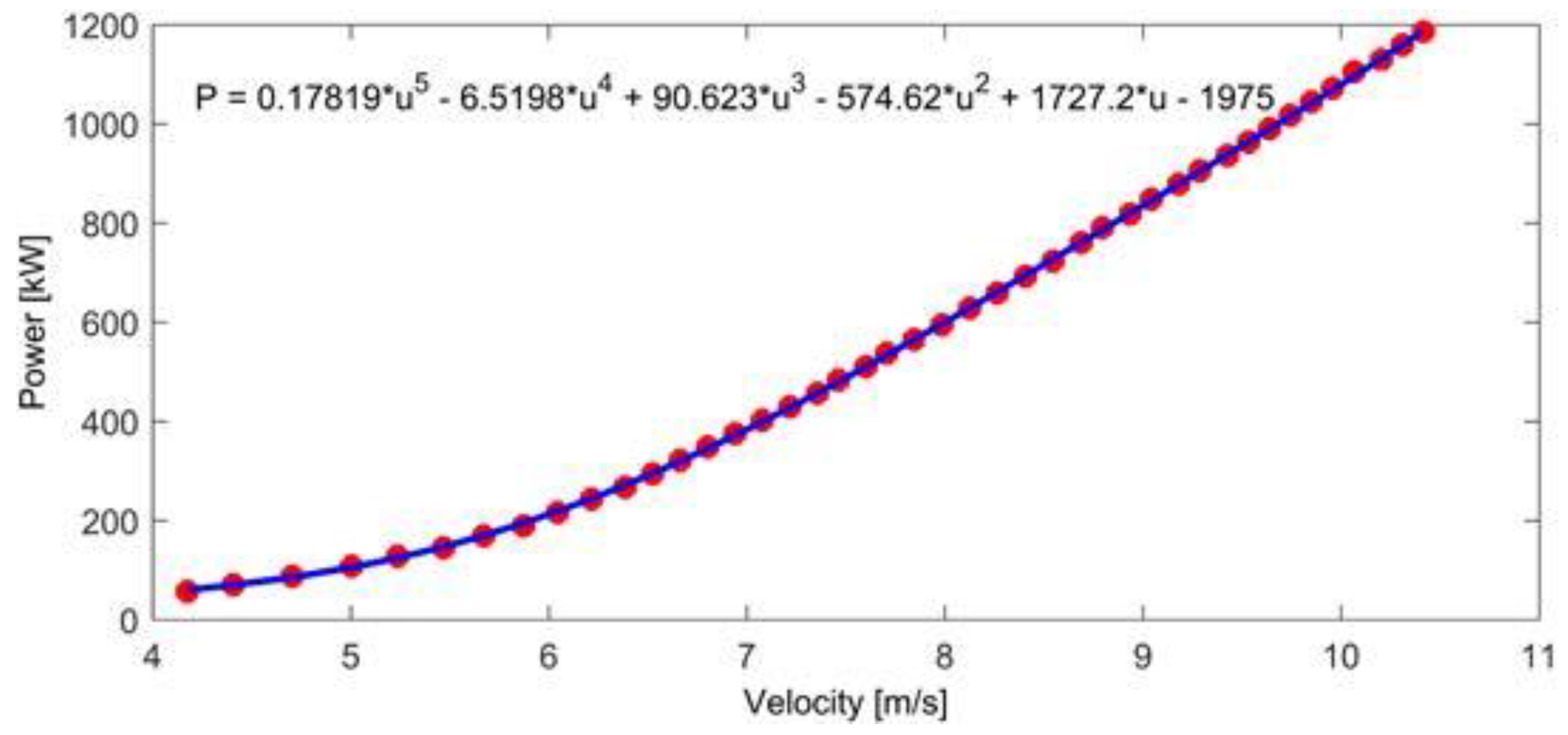
The power curve, which gives the power production as a function of incoming wind speed, is used to predict the power generated by each turbine. Here, the data available for Vestas V-80 wind turbines is used where a fifth degree polynomial is fitted to the data, as shown in Figure 2.
3. Case Description
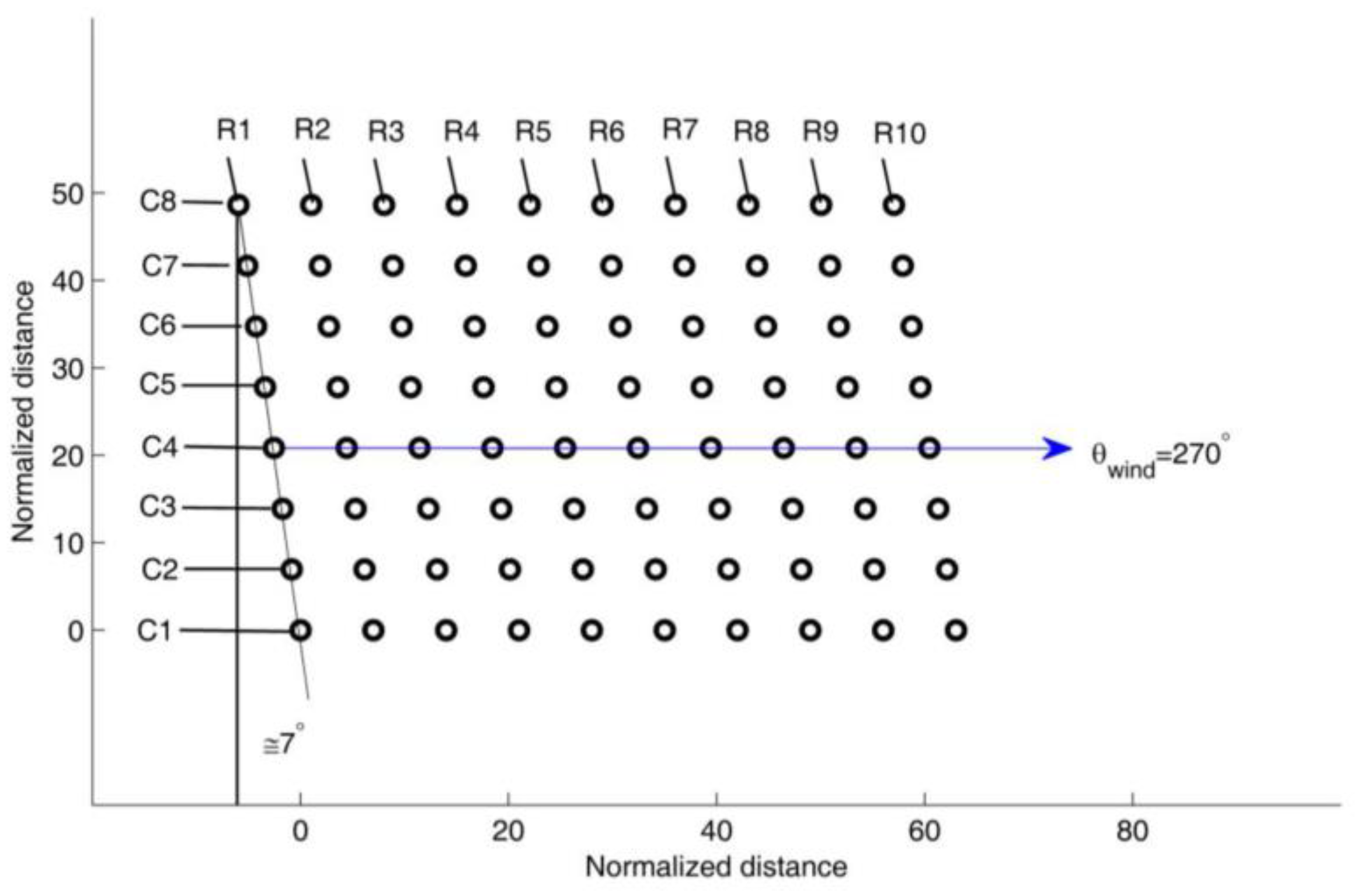
We selected the Horns Rev offshore wind farm as a case study because LES flow and power predictions [26,36] and power measurements [17,37] are available to evaluate the performance of the proposed analytical wind farm model. The wind farm has a total rated power capacity of 160 MW and consists of eighty Vestas V-80 wind turbines within an area of approximately 20 km2. It is located in the North Sea, approximately 15 km off the westernmost point of Denmark. Each turbine has a rotor diameter of and a hub height of (above sea level). Figure 3 shows a schematic of the Horns Rev wind farm layout. The wind farm has a rhomboid shape with wind turbines arranged in 8 columns (aligned with the East-West direction) and 10 rows (turned approximately 7° counterclockwise from the North-South direction). The turbines are regularly spaced, with a minimum spacing between two consecutive turbines of 7 rotor diameters.
The wind turbine power curve and thrust coefficient curve, both of which are inputs required by the new analytical wind farm model, are typically available from the manufacturer. The curves for the Vestas V-80 turbine are shown in Figure 4. The same curves were also used by Wu and Porté-Agel [36] in their LES study of wake flows in the Horns Rev wind farm. To specify the incoming flow conditions, the aerodynamic surface roughness of the sea surface was set to . The inflow wind condition is characterized by a turbulence intensity of 7.7% at the hub height and an average velocity of 8 at the same height. These conditions are the same as those for the available power measurements [17], LES flow, and power results [36].
4. Results and Discussion
In this section, predictions obtained with the new analytical model for the turbine wakes and associated power losses in the Horns Rev wind farm are presented. The results are also compared with available power measurements [17,37] and LES data [26,36], as well as with predictions from an existing analytical top-hat wake model. The top-hat wake model is based on the one proposed by Katic et al. [6] and is commonly used in a variety of software (e.g., the Wind Atlas Analysis and Application Program (WAsP) and the PARK model). In this top-hat wake model, the wake growth rate is set to a constant (and spatially uniform) value of 0.04, which is based on the formula proposed by Frandsen et al. [14].
The simulated total normalized power output from the Horns Rev wind farm calculated with the new model, LES [26], and the top-hat model [6] is shown in Figure 5 for a wide range of wind directions (from to ). This enables an extensive model evaluation over a variety of both full-wake and partial-wake operating conditions. Furthermore, we normalize the simulated power output by the power of an equivalent number of stand-alone wind turbines operating in the same incoming wind condition. As shown in Figure 1, a good agreement is found between the proposed analytical model and LES, while the top-hat model significantly under predicts the normalized power. Furthermore, wind farm power production substantially decreases (approximately 30%) as the wind farm is exposed to wind direction angles (, , and ), corresponding to full-wake conditions with short streamwise distances between consecutive wind turbines. Additionally, when the wind farm is exposed to the wind directions in which there is a large streamwise distance between turbines (e.g., and ), several local maxima can be distinguished.
Next, the performance of different multiple wake superposition approaches is evaluated. For this purpose, we compare the normalized power output simulated with the new analytical model using both velocity deficit superposition (i.e., Equation (12)) and energy deficit superposition (i.e., Equation (8)) with the one obtained with LES. The normalized power output as a function of turbine row (averaged over columns 2, 3, and 4) in the wind farm is shown in Figure 2. The difference between the inflow velocity at the turbine and the wake velocity is used for calculation of the velocity and energy deficits. It is important to mention that if the difference between the incoming velocity to the turbine and the wake velocity is used, unrealistic negative velocities can occur as a result of a large number of turbine rows. As shown in Figure 6, although energy deficit superposition substantially overestimates the normalized power output, velocity deficit superposition shows good agreement with LES.
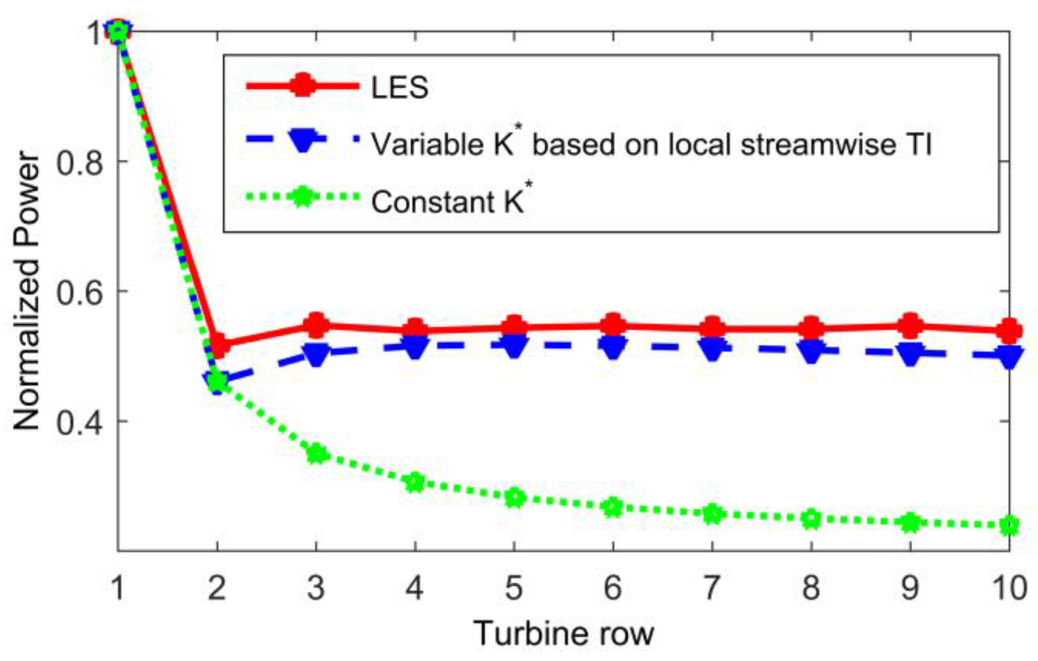
To show the impact of the local wake growth rate on wind farm power prediction, the simulated normalized power output obtained using constant and variable wake growth rates (the latter calculated based on the local streamwise turbulence intensity, Equation (15)) is compared with LES. As shown in Figure 7, reasonable agreement between the analytical model and LES can be achieved using a variable wake growth rate. In contrast, assuming a constant wake growth rate leads to a clear underestimation of the normalized power output. This is because, inside the wind farm, the wakes recover faster (and thus have a larger growth rate) due to the increased flow entrainment induced by the relatively higher turbulence levels in the wakes, compared with the incoming flow. Our results show the importance of taking into account the increased level of turbulence intensity and the associated increased growth rate for the prediction of wakes and power inside wind farms.
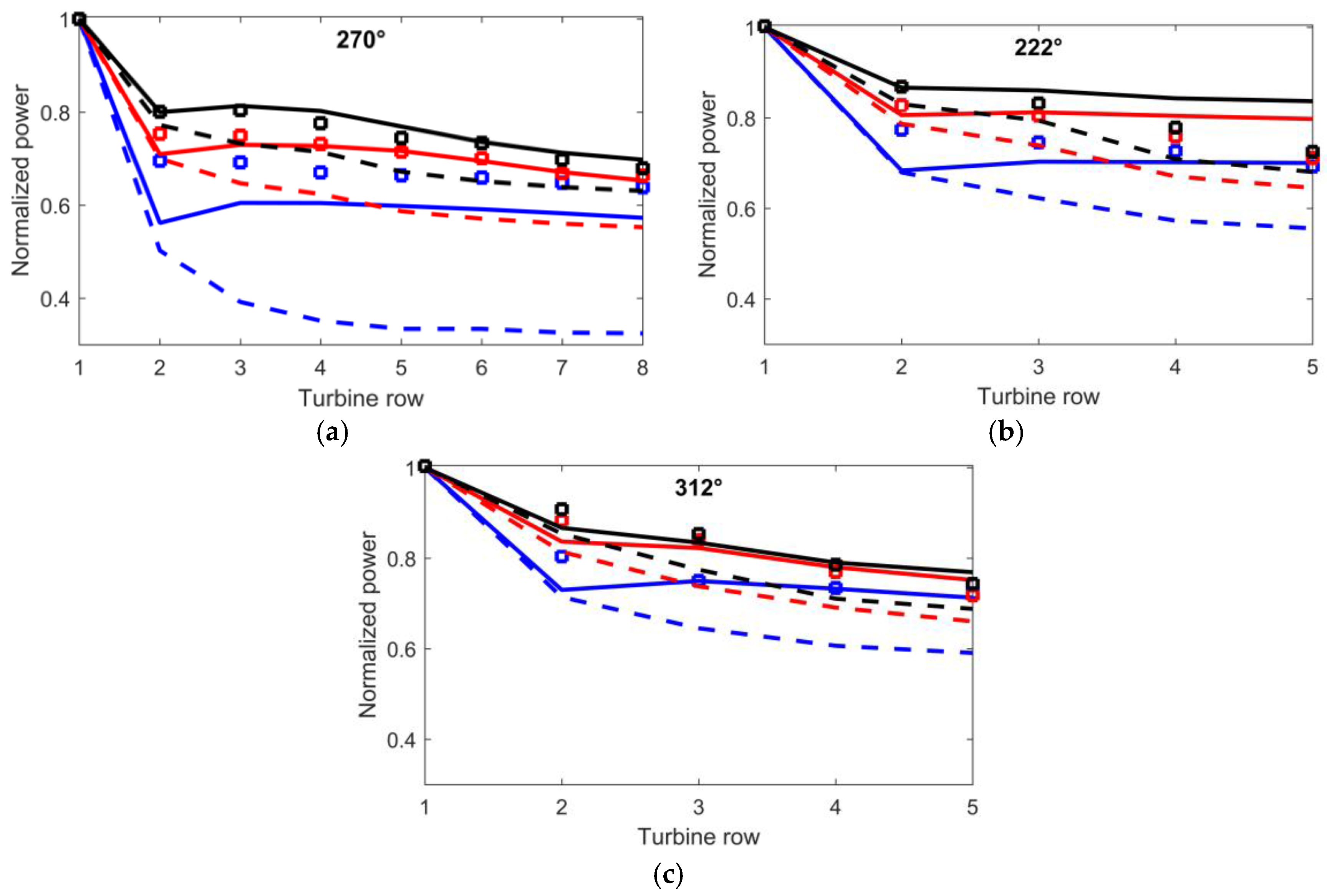
Figure 8 shows the normalized power output for three wind sectors (i.e., ±5°, ±10°, and ±15°) centered on three mean wind directions ( = 270°, 222°, and 312°) simulated by the new analytical model and WAsP, as well as the measurements [37]. As shown in this figure, WAsP clearly tends to under predict the power output, while a very good agreement between the measurements and the proposed model is found. This result reveals the fact that considering a top-hat shape for normalized velocity deficit can lead to substantial error in both full-wake and partial-wake conditions.
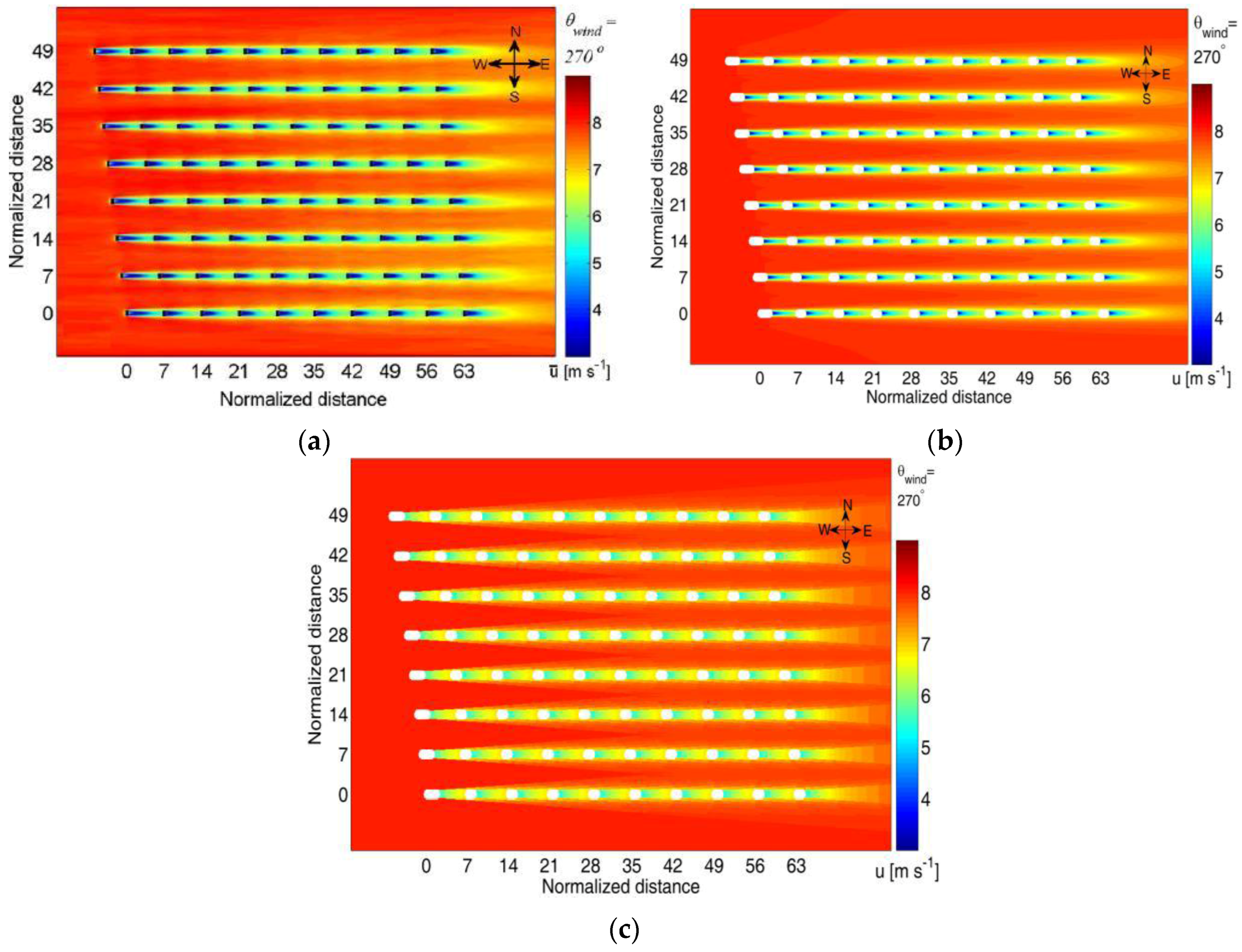
One of the main features of the new analytical wind farm model is the capability of computing the mean velocity field inside a wind farm and the associated power output in a computationally efficient way while keeping the accuracy acceptable. Figure 9 shows a two-dimensional contour plot of the streamwise velocity on a horizontal plane at hub level simulated by LES [26,36], the new analytical model, and the classical top-hat analytical model [6]. It should be mentioned that the analytical wake models can only predict the velocity deficit in the far-wake region (after a downwind distance of approximately two rotor diameters from each turbine) where the wake flows have a self-similar Gaussian behavior and can be described by global parameters such as the thrust coefficient. To this effect, a white rectangle is placed in the near wake region in Figure 9. Reasonable agreement between the proposed analytical model and LES is found, while the top-hat model gives a less realistic prediction of the velocity flow field due to the top-hat assumption for the velocity deficit, which results in a uniform wake velocity distribution in the spanwise direction. Furthermore, it is obvious that wake flows are responsible for a significant reduction of the velocity immediately upstream of the wind turbines inside the wind farm.
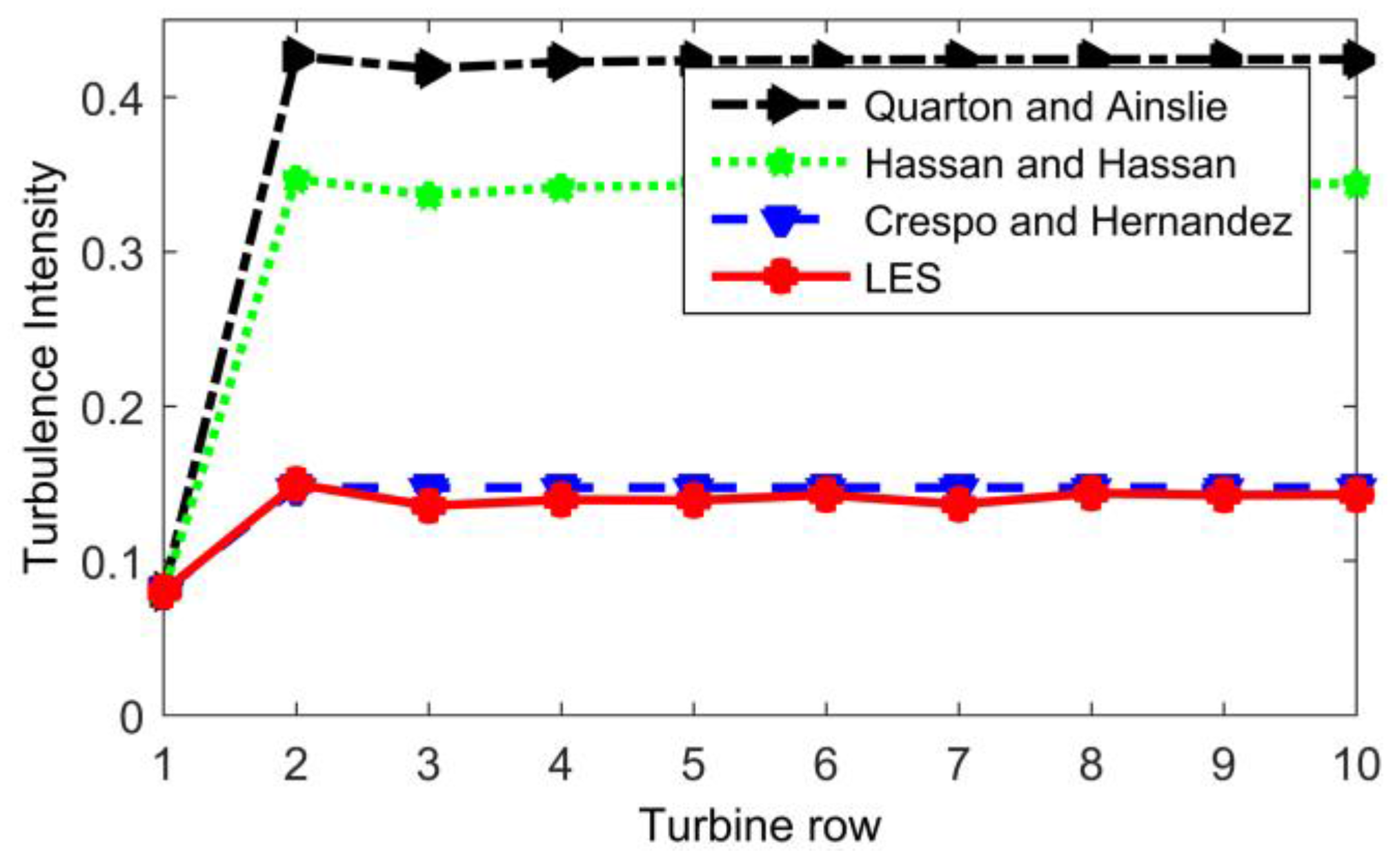
As discussed previously, the wake growth rate is dependent on the local streamwise turbulence intensity. Therefore, the local streamwise turbulence intensity in the wind farm should be predicted in the analytical wind farm model. Furthermore, it is imperative to estimate the level of turbulence intensity at the turbine locations to investigate the impact of fatigue loading due to turbulence on the turbines. Figure 10 presents the level of streamwise turbulence intensity at hub height in the wind farm obtained from the models of Quarton and Ainslie [30], Hassan and Hassan [31], and Crespo and Hernandez [32], as well as the LES predictions. It clearly shows that both the models of Quarton and Ainslie and of Hassan and Hassan over predict the level of streamwise turbulence intensity when compared with LES. In contrast, the model of Crespo and Hernandez, which is used in the new proposed model, predicts turbulence intensity levels that are very similar to those simulated by LES.
5. Conclusions
A new analytical wind-farm wake model is proposed to predict wake flows and associated power losses inside wind farms. The model combines the self-similar Gaussian model recently developed by Bastankhah and Porté-Agel [15] for stand-alone wind turbine wakes with a new wake superposition procedure that is based on the superposition of velocity deficits. This combination guarantees that mass and momentum are conserved by the model. The growth rate of each individual wake needs to be specified and is computed using an empirical expression based on the local streamwise turbulence intensity, which is predicted inside the wind farm using the model proposed by Crespo and Hernandes [32]. Finally, the power curve of the wind turbines is used to estimate the power production.
The Horns Rev wind farm was selected as a validation case study because power measurements and previous LES predictions of the wake flows and turbine power are available for a wide range of inflow conditions. Comparison between the measurements and LES results reveal that the new analytical wind-farm model yields reasonably accurate predictions of the power output from the Horns Rev wind farm for all of the wind directions considered in this study. Additionally, we show that the power prediction of the new analytical wind farm model is significantly better than the one estimated by WAsP.
Future research will consider the development of more general parametrization of the local turbulence intensity and the wake growth rate, which can then be used by the new model for a wider range of inflow characteristics (e.g., including thermal stability) and turbine operation conditions (e.g., turbine down-regulation or yawing). Furthermore, because of its low computational cost, the newly proposed model can be used for the optimization of wind farm layouts to maximize power output and minimize the fatigue load on the wind turbines.
Acknowledgments
This research was supported by the Swiss National Science Foundation (grant 200021-132122), the Swiss Innovation and Technology Committee (CTI) and the Swiss Federal Office of Energy (OFEN) within the context of the Swiss Competence Center for Energy Research ‘FURIES: Future Swiss Electrical Infrastructure’. The authors also thank Yu-Ting Wu for providing the WAsP data.
Author Contributions
This study was done as Amin Niayifar’s internship at Wind Engineering and Renewable Energy Laboratory (WIRE) supervised by Fernando Porté-Agel.
Conflicts of Interest
The authors declare no conflict of interest.
References
- Globalwind Energy Council. Globalwind Report: Annual Market Update 2012. Available online: Http://www.Gwec.Net/wp-content/uploads/2012/06/annual report 2012 lowres.pdf (accessed on 30 June 2013).
- Barthelmie, R.J.; Pryor, S.; Frandsen, S.T.; Hansen, K.S.; Schepers, J.; Rados, K.; Schlez, W.; Neubert, A.; Jensen, L.; Neckelmann, S. Quantifying the impact of wind turbine wakes on power output at offshore wind farms. J. Atmos. Oceanic Technol. 2010, 27, 1302–1317. [Google Scholar] [CrossRef]
- Crespo, A.; Hernandez, J.; Frandsen, S. Survey of modelling methods for wind turbine wakes and wind farms. Wind Energy 1999, 2, 1–24. [Google Scholar] [CrossRef]
- Chowdhury, S.; Zhang, J.; Messac, A.; Castillo, L. Optimizing the arrangement and the selection of turbines for wind farms subject to varying wind conditions. Renew. Energy 2013, 52, 273–282. [Google Scholar] [CrossRef]
- Lissaman, P.B.S. Energy effectiveness of arbitrary arrays of wind turbines. J. Energy 1979, 3, 323–328. [Google Scholar] [CrossRef]
- Katic, I.; Højstrup, J.; Jensen, N. A Simple Model for Cluster Efficiency. In Proceedings of the European Wind Energy Association Conference and Exhibition, Rome, Italy, 1986; pp. 407–410.
- Frandsen, S. On the wind speed reduction in the center of large clusters of wind turbines. J. Wind Eng. Ind. Aerodyn. 1992, 39, 251–265. [Google Scholar] [CrossRef]
- Calaf, M.; Meneveau, C.; Meyers, J. Large eddy simulation study of fully developed wind-turbine array boundary layers. Phys. Fluids 2010, 22, 015110. [Google Scholar] [CrossRef]
- Abkar, M.; Porté-Agel, F. The effect of free-atmosphere stratification on boundary-layer flow and power output from very large wind farms. Energies 2013, 6, 2338–2361. [Google Scholar] [CrossRef]
- Stevens, R.J.; Gayme, D.F.; Meneveau, C. Coupled wake boundary layer model of wind-farms. J. Renew. Sustain. Energy 2015, 7, 023115. [Google Scholar] [CrossRef]
- Stevens, R.J.; Gayme, D.F.; Meneveau, C. Generalized coupled wake boundary layer model: Applications and comparisons with field and les data for two wind farms. Wind Energy 2016. [Google Scholar] [CrossRef]
- Jensen, N.O. A Note on Wind Generator Interaction; Technical report Ris-M-2411; Risø National Laboratory: Roskilde, Denmark, 1983. [Google Scholar]
- Voutsinas, S.; Rados, K.; Zervos, A. On the analysis of wake effects in wind parks. Wind Eng. 1990, 14, 204–219. [Google Scholar]
- Frandsen, S.; Barthelmie, R.; Pryor, S.; Rathmann, O.; Larsen, S.; Højstrup, J.; Thøgersen, M. Analytical modelling of wind speed deficit in large offshore wind farms. Wind Energy 2006, 9, 39–53. [Google Scholar] [CrossRef]
- Bastankhah, M.; Porté-Agel, F. A new analytical model for wind-turbine wakes. Renew. Energy 2014, 70, 116–123. [Google Scholar] [CrossRef]
- González, J.S.; Rodriguez, A.G.G.; Mora, J.C.; Santos, J.R.; Payan, M.B. Optimization of wind farm turbines layout using an evolutive algorithm. Renew. Energy 2010, 35, 1671–1681. [Google Scholar] [CrossRef]
- Barthelmie, R.; Larsen, G.; Frandsen, S.; Folkerts, L.; Rados, K.; Pryor, S.; Lange, B.; Schepers, G. Comparison of wake model simulations with offshore wind turbine wake profiles measured by sodar. J. Atmos. Oceanic Technol. 2006, 23, 888–901. [Google Scholar] [CrossRef]
- Crasto, G.; Gravdahl, A.; Castellani, F.; Piccioni, E. Wake modeling with the actuator disc concept. Energy Procedia 2012, 24, 385–392. [Google Scholar] [CrossRef]
- Garrad Hassan and Partners Ltd. GH Windfarmer Theory Manual; Garrad Hassan and Partners Ltd.: Bristol, UK, 2009. [Google Scholar]
- Openwind Theoretical Basis and Validation; AWS Truepower, LCC: Albany, NY, USA, 2010.
- Thogersen, M.L.; Sorensen, T.; Nielsen, P.; Grotzner, A.; Chun, S. Introduction to Wind Turbine Wake Modelling and Wake Generated Turbulence; Risø National Laboratory, EMD International A/S: Aalborg, Denmark, 2006. [Google Scholar]
- Chamorro, L.P.; Porté-Agel, F. A wind-tunnel investigation of wind-turbine wakes: Boundary-layer turbulence effects. Boundary-Layer Meteorol. 2009, 132, 129–149. [Google Scholar] [CrossRef]
- Wu, Y.-T.; Porté-Agel, F. Atmospheric turbulence effects on wind-turbine wakes: An les study. Energies 2012, 5, 5340–5362. [Google Scholar] [CrossRef]
- Xie, S.; Archer, C. Self-similarity and turbulence characteristics of wind turbine wakes via large-eddy simulation. Wind Energy 2015, 18, 1815–1838. [Google Scholar] [CrossRef]
- Abkar, M.; Porté-Agel, F. Influence of atmospheric stability on wind-turbine wakes: A large-eddy simulation study. Phys. Fluids 2015, 27, 035104. [Google Scholar] [CrossRef]
- Porté-Agel, F.; Wu, Y.-T.; Chen, C.-H. A numerical study of the effects of wind direction on turbine wakes and power losses in a large wind farm. Energies 2013, 6, 5297–5313. [Google Scholar] [CrossRef]
- Abkar, M.; Porté-Agel, F. Mean and turbulent kinetic energy budgets inside and above very large wind farms under conventionally-neutral condition. Renew. Energy 2014, 70, 142–152. [Google Scholar] [CrossRef]
- Abkar, M.; Sharifi, A.; Porté-Agel, F. Wake flow in a wind farm during a diurnal cycle. J. Turbulence 2016, 17, 1–22. [Google Scholar] [CrossRef]
- Porté-Agel, F.; Wu, Y.-T.; Lu, H.; Conzemius, R.J. Large-eddy simulation of atmospheric boundary layer flow through wind turbines and wind farms. J. Wind Eng. Ind. Aerodyn. 2011, 99, 154–168. [Google Scholar] [CrossRef]
- Quarton, D.; Ainslie, J. Turbulence in wind turbine wakes. Wind Eng. 1990, 14, 15–23. [Google Scholar]
- Hassan, U.; Hassan, G. A Wind Tunnel Investigation of the Wake Structure within Small Wind Turbine Farms; Harwell Laboratory, Energy Technology Support Unit: Brighton, UK, 1993. [Google Scholar]
- Crespo, A.; Hernandez, J. Turbulence characteristics in wind-turbine wakes. J. Wind Eng. Ind. Aerodyn. 1996, 61, 71–85. [Google Scholar] [CrossRef]
- Vermeulen, P. An Experimental Analysis of Wind Turbine Wakes. In Proceedings of the International Symposium on Wind Energy Systems, Copenhagen, Denmark, 26–29 August 1980; pp. 431–450.
- Abkar, M.; Porté-Agel, F. A new wind-farm parameterization for large-scale atmospheric models. J. Renew. Sustain. Energy 2015, 7, 013121. [Google Scholar] [CrossRef]
- Frandsen, S.; Thogersen, M.L. Integrated fatigue loading for wind turbines in wind farms by combining ambient turbulence and wakes. Wind Eng. 1999, 23, 327–340. [Google Scholar]
- Wu, Y.-T.; Porté-Agel, F. Modeling turbine wakes and power losses within a wind farm using les: An application to the horns rev offshore wind farm. Renew. Energy 2015, 75, 945–955. [Google Scholar] [CrossRef]
- Barthelmie, R.J.; Hansen, K.; Frandsen, S.T.; Rathmann, O.; Schepers, J.; Schlez, W.; Phillips, J.; Rados, K.; Zervos, A.; Politis, E. Modelling and measuring flow and wind turbine wakes in large wind farms offshore. Wind Energy 2009, 12, 431–444. [Google Scholar] [CrossRef]
Figure 1.
Wake growth rate for the V-80 turbine in boundary layer flow with different streamwise turbulence intensities at hub height.
Figure 1.
Wake growth rate for the V-80 turbine in boundary layer flow with different streamwise turbulence intensities at hub height.
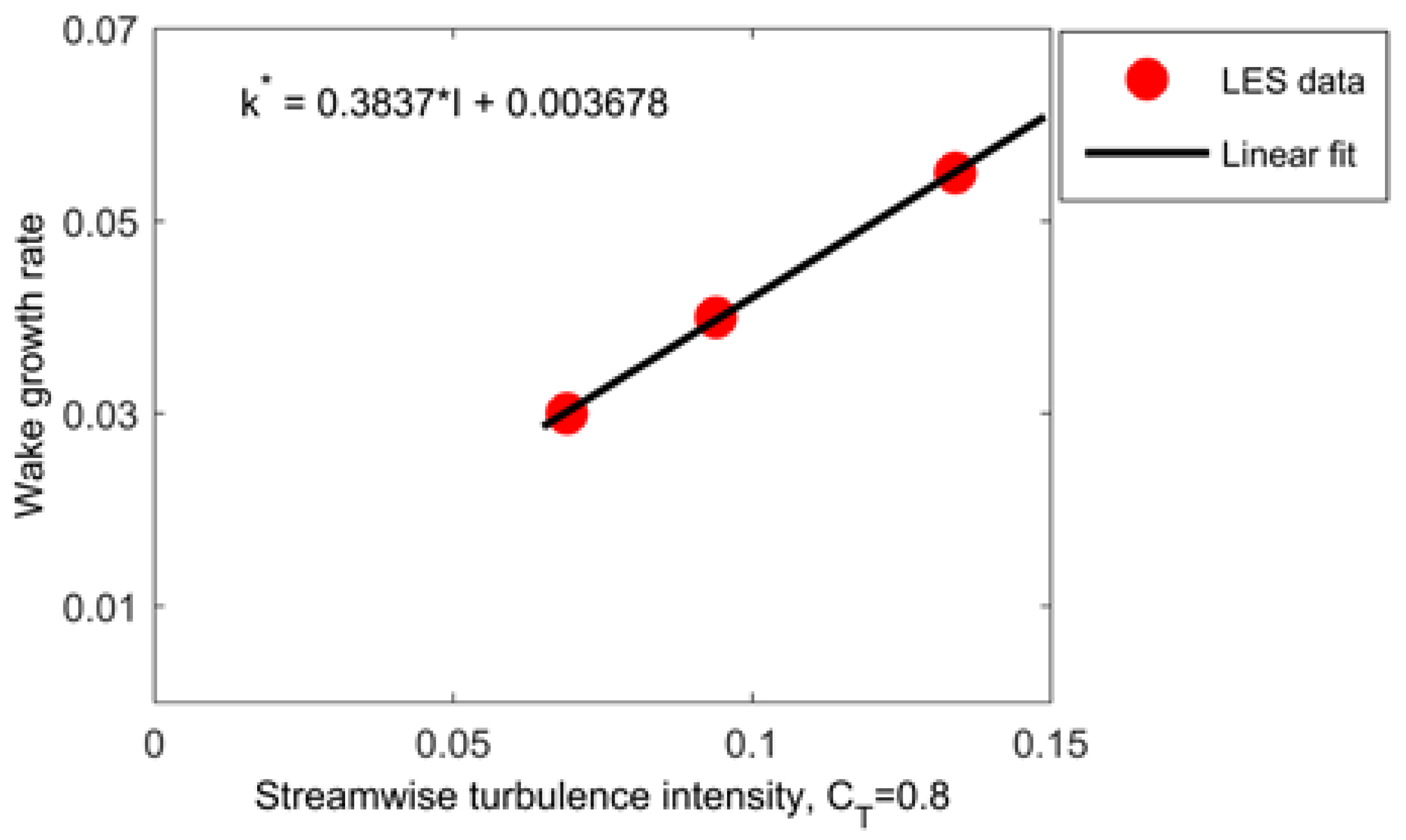
Figure 2.
Power curve of the V-80 wind turbine. Red circles correspond to the manufacturer’s data and the blue line represents a polynomial fit.
Figure 2.
Power curve of the V-80 wind turbine. Red circles correspond to the manufacturer’s data and the blue line represents a polynomial fit.

Figure 3.
Layout of the Horns Rev wind farm. Distances are normalized by the rotor diameter .

Figure 4.
Measured and simulated power curve and thrust coefficient curve of the Vestas V-80 2 MW wind turbine, for a range of wind speeds (Source: Wu and Porté-Agel, 2014).
Figure 4.
Measured and simulated power curve and thrust coefficient curve of the Vestas V-80 2 MW wind turbine, for a range of wind speeds (Source: Wu and Porté-Agel, 2014).
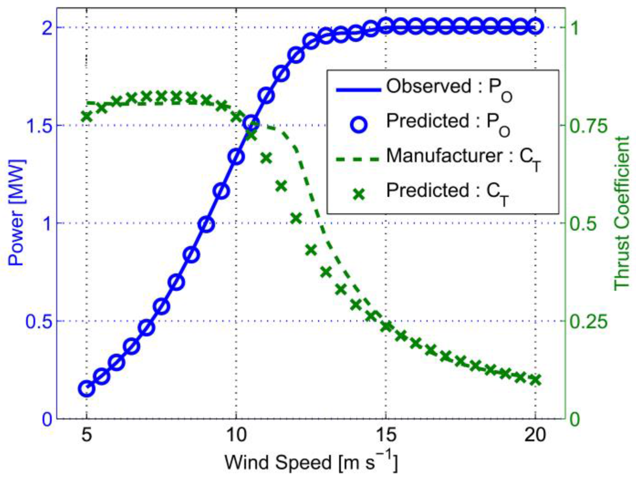
Figure 5.
Distribution of the normalized Horns Rev wind farm power output obtained with the new analytical model and LES for different wind directions.
Figure 5.
Distribution of the normalized Horns Rev wind farm power output obtained with the new analytical model and LES for different wind directions.
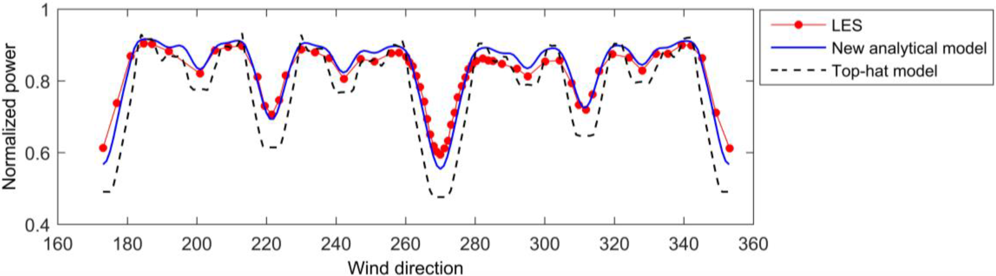
Figure 6.
Comparison of the wind-farm power output for obtained using LES as well as the new analytical model with both energy and velocity deficit superpositions.
Figure 6.
Comparison of the wind-farm power output for obtained using LES as well as the new analytical model with both energy and velocity deficit superpositions.
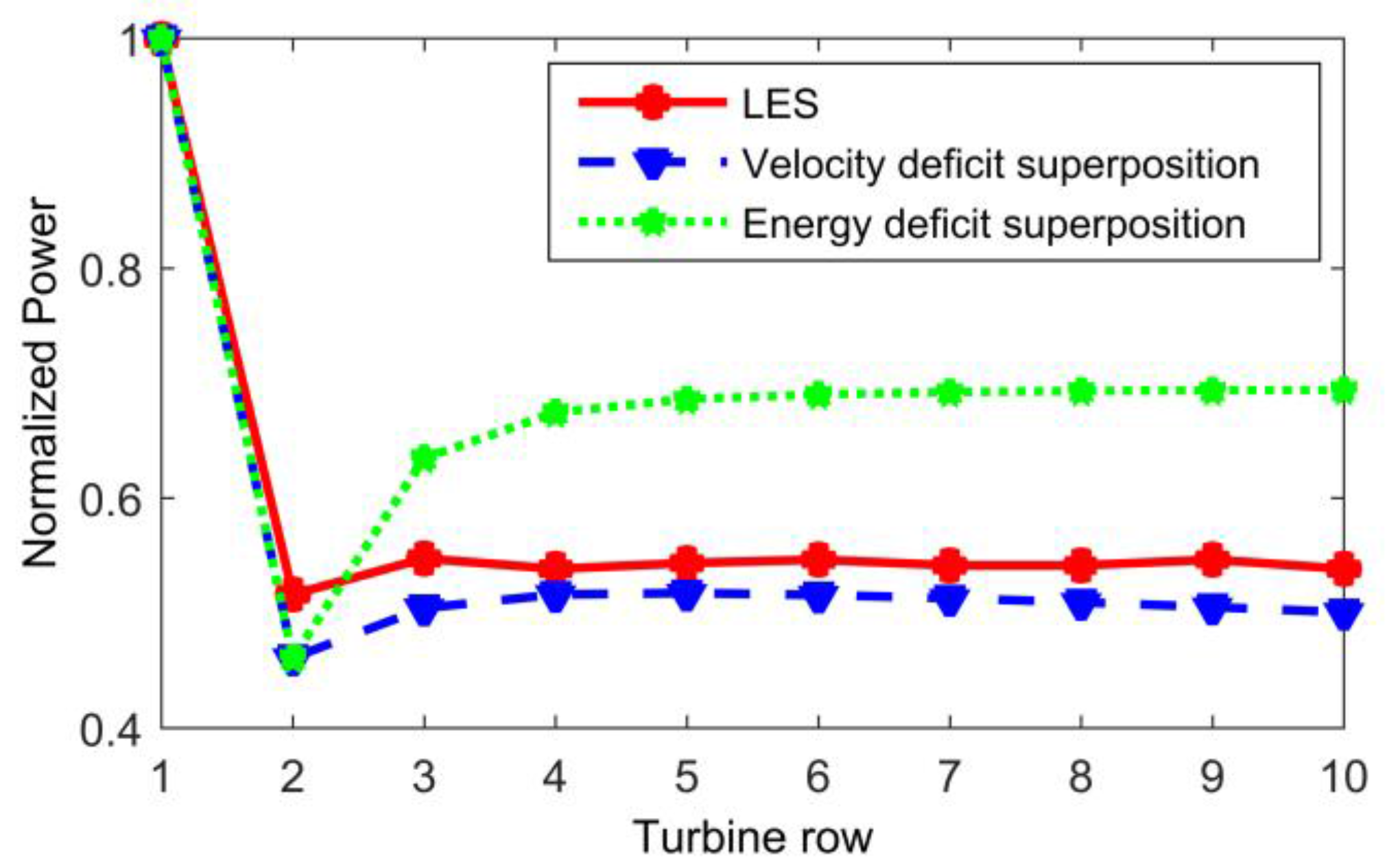
Figure 7.
Comparison of the power output for = 270° obtained with the new analytical model using a constant wake growth rate and a variable wake growth rate based on the local streamwise turbulence intensity.
Figure 7.
Comparison of the power output for = 270° obtained with the new analytical model using a constant wake growth rate and a variable wake growth rate based on the local streamwise turbulence intensity.

Figure 8.
Comparison of the simulated and observed power output centered on three mean wind directions = 270° (a); 222° (b) and 312° (c). Symbols, lines, and dashed lines denote the observed, new analytical model, and WAsP data, respectively. Blue, red, and black colors represent ±5°, ±10°, and ±15° wind sectors, respectively.

Figure 9.
Comparison of the time-averaged streamwise velocity at a horizontal plane at hub height: (a) LES; (b) new analytical model and (c) top-hat model.
Figure 9.
Comparison of the time-averaged streamwise velocity at a horizontal plane at hub height: (a) LES; (b) new analytical model and (c) top-hat model.

Figure 10.
Comparison of the streamwise turbulence intensity at hub height immediately upstream of each turbine row, obtained with LES and three simple models.
Figure 10.
Comparison of the streamwise turbulence intensity at hub height immediately upstream of each turbine row, obtained with LES and three simple models.
© 2016 by the authors; licensee MDPI, Basel, Switzerland. This article is an open access article distributed under the terms and conditions of the Creative Commons Attribution (CC-BY) license (http://creativecommons.org/licenses/by/4.0/).
Share and Cite
MDPI and ACS Style
Niayifar, A.; Porté-Agel, F. Analytical Modeling of Wind Farms: A New Approach for Power Prediction. Energies 2016, 9, 741. https://doi.org/10.3390/en9090741
AMA Style
Niayifar A, Porté-Agel F. Analytical Modeling of Wind Farms: A New Approach for Power Prediction. Energies. 2016; 9(9):741. https://doi.org/10.3390/en9090741
Chicago/Turabian StyleNiayifar, Amin, and Fernando Porté-Agel. 2016. "Analytical Modeling of Wind Farms: A New Approach for Power Prediction" Energies 9, no. 9: 741. https://doi.org/10.3390/en9090741
Note that from the first issue of 2016, this journal uses article numbers instead of page numbers. See further details here.