
Adaptive Hybrid Fuzzy-Proportional Plus Crisp-Integral Current Control Algorithm for Shunt Active Power Filter Operation

 , ,
, ,
Abstract
:1. Introduction
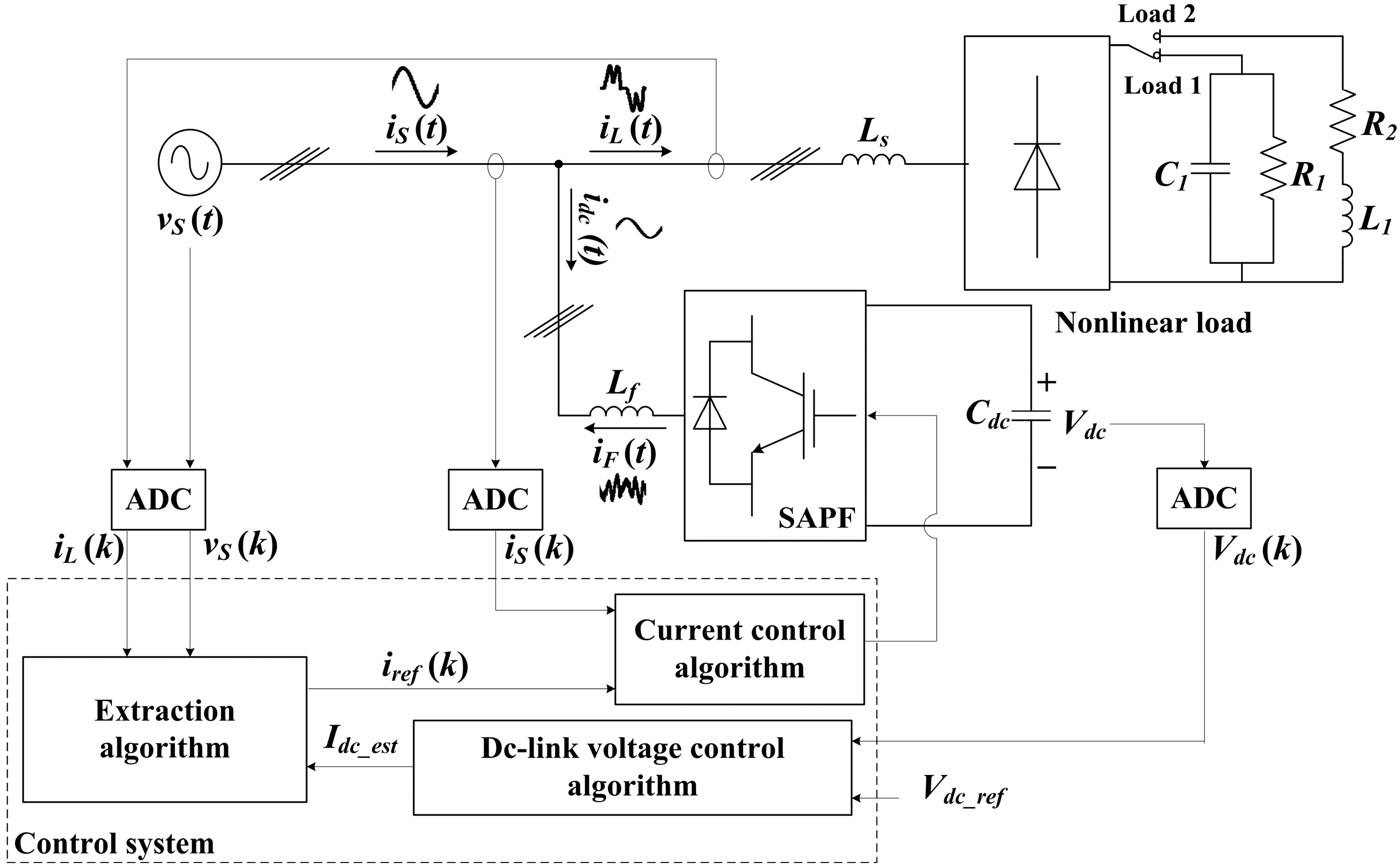
2. Principle Operation of Shunt Active Power Filter
3. Proposed Adaptive Hybrid Fuzzy-Proportional Plus Crisp-Integral Current Control Algorithm
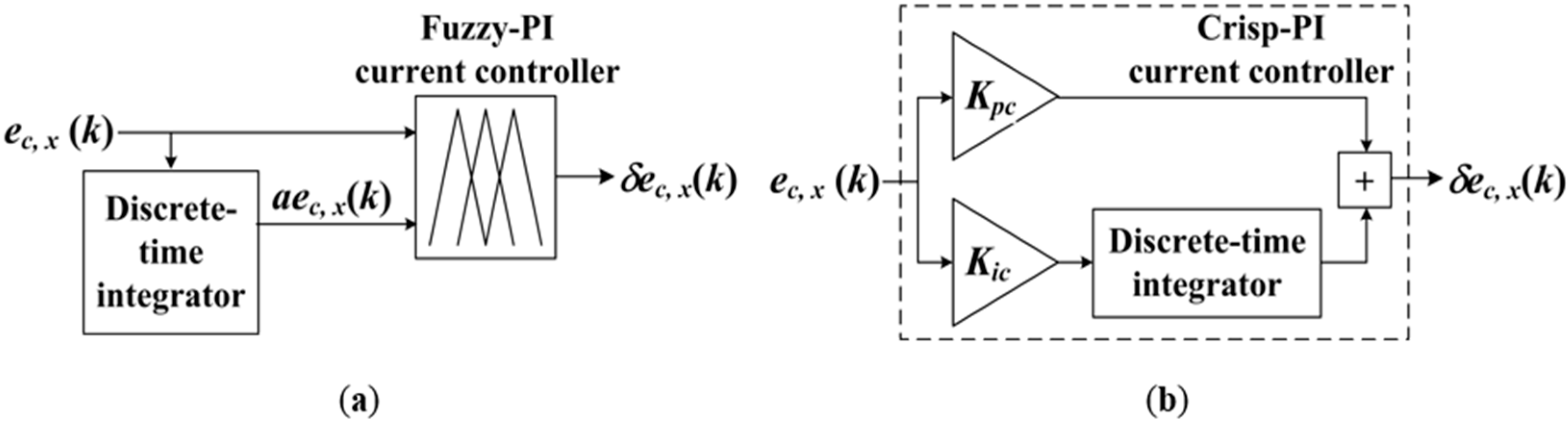
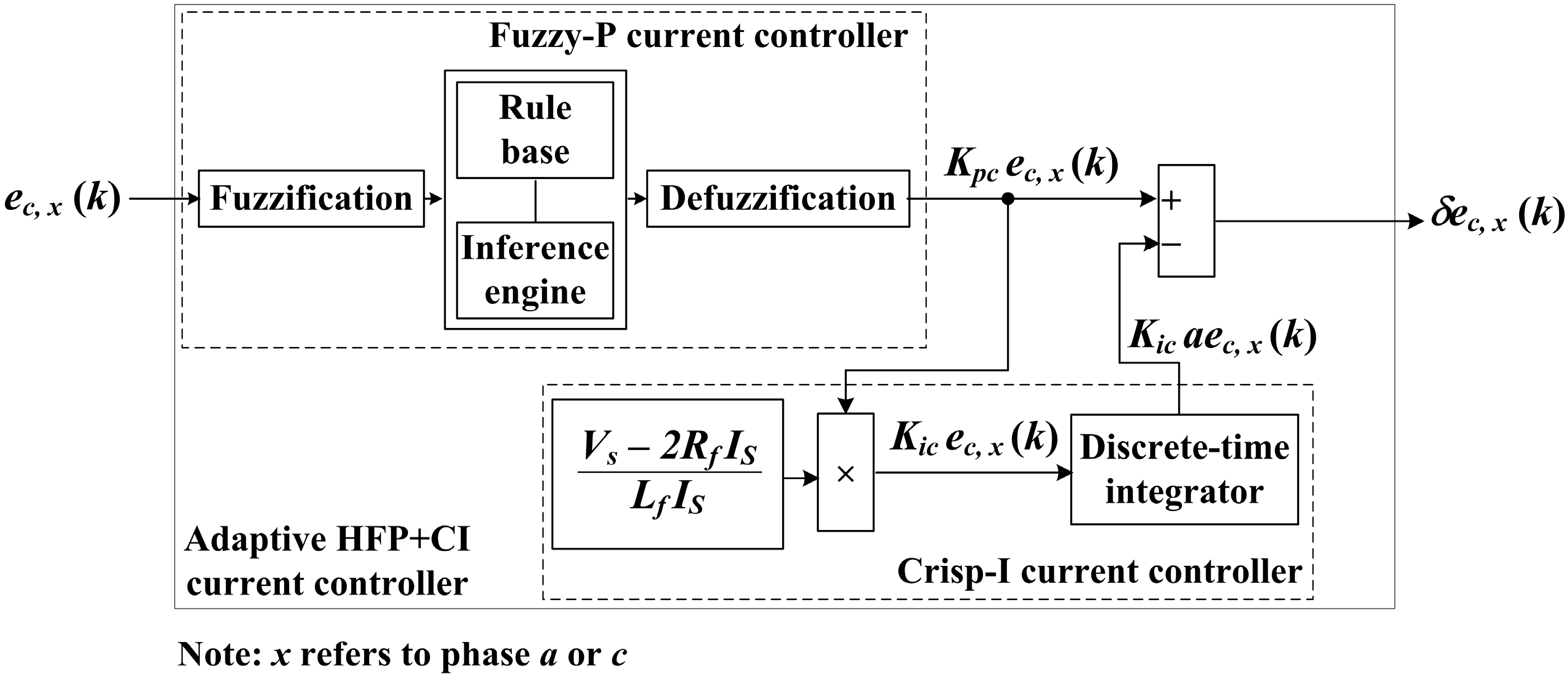
3.1. Proposed Adaptive Hybrid Fuzzy-Proportional Plus Crisp-Integral Current Controllers
- For the MF set of :The boundary is determined based on the response of the proposed CCA during the open-loop operation.
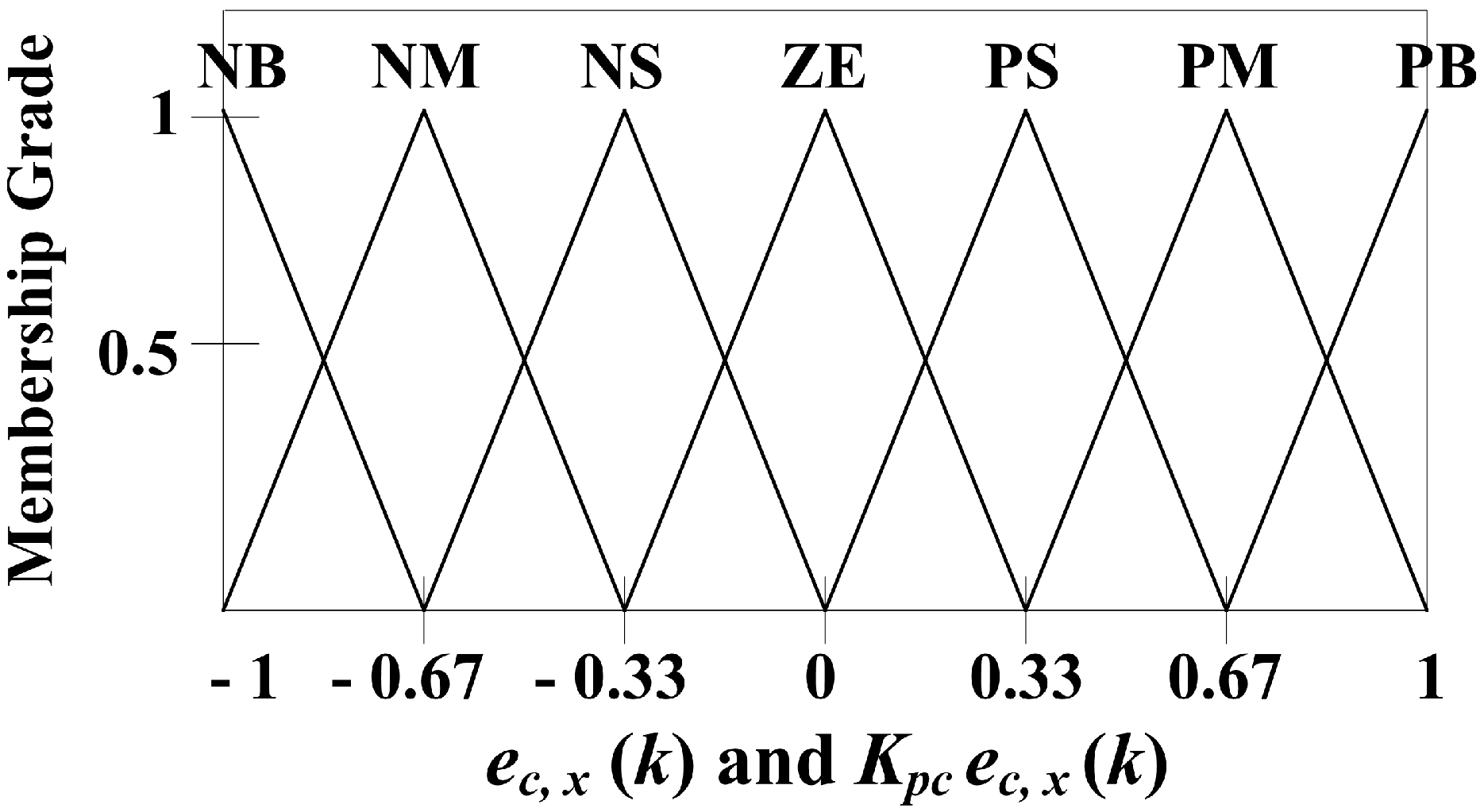
- For the MF set of :The boundary is determined based on the total harmonic distortion (THD) value of . At this moment, the SAPF applies a fixed supply; for eliminating the effect of the operation of the dc-link VCA. Thus, Equation (1) becomes:Then, the rule base implements SISO fuzzy rules; for simplifying the controller structure. It is developed based on the relationship between and , and the relationship between and . Both relationships can be expressed as in Equations (3) and (5); they can easily be interpreted in linguistic reasoning. Since the shape of remains unchanged throughout the compensation process, therefore the rule base is developed as follows:
- If is positive:is higher than . Then, is reduced by increasing . Hence, is positive.
- If is negative:is lower than . Then, is increased by decreasing . Hence, is negative.
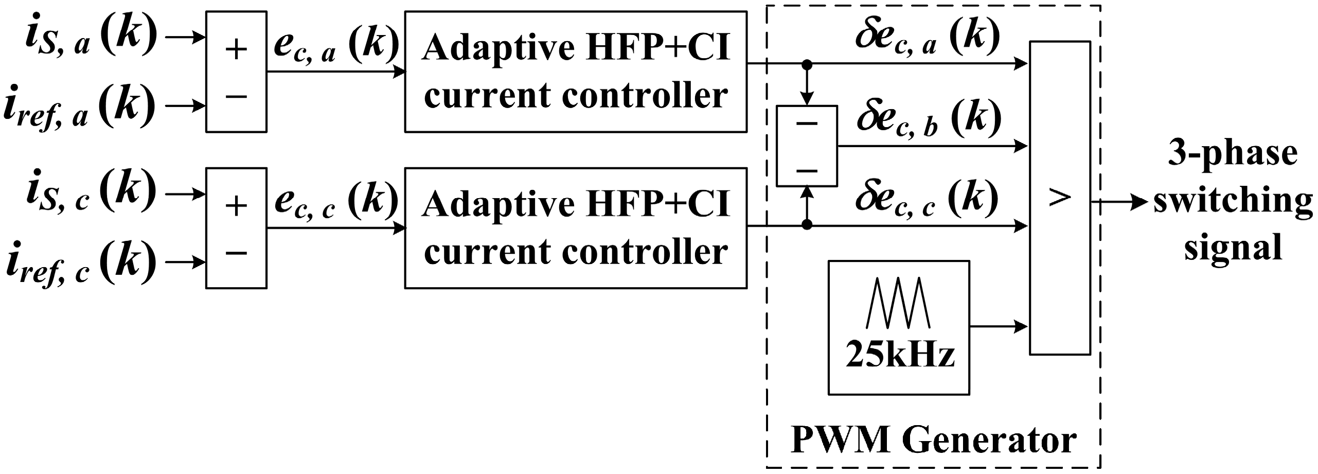
3.2. Pulse Width Modulation Generator
- If is greater than the carrier signal, then the switching signal equals to 1.
- If is lower than the carrier signal, then the switching signal equals to 0.
4. Simulation Work
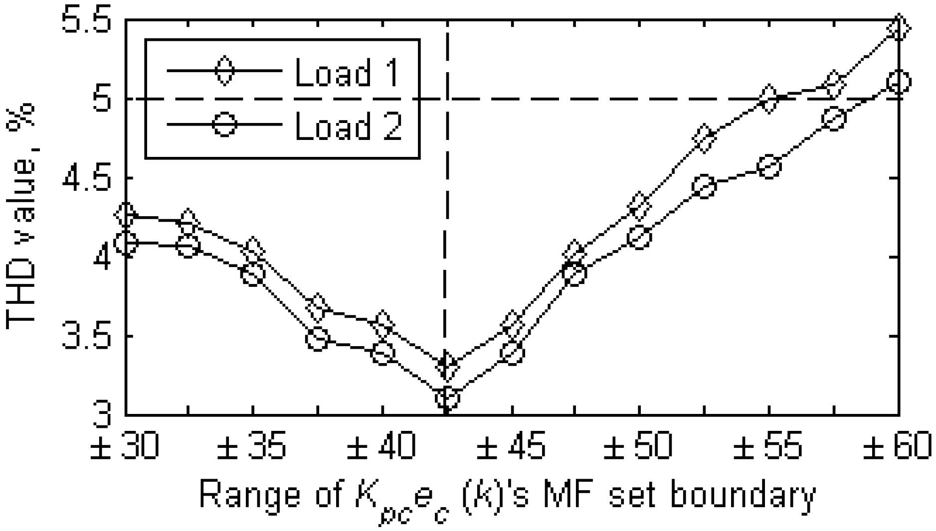
4.1. Selection of the Range of ’s Membership Function Set Boundary
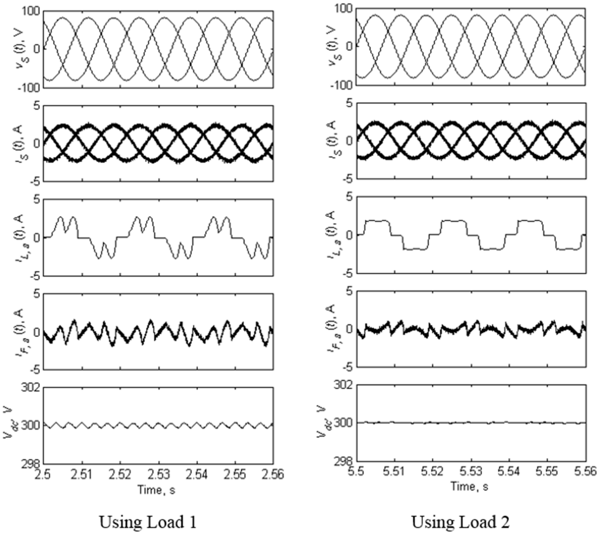
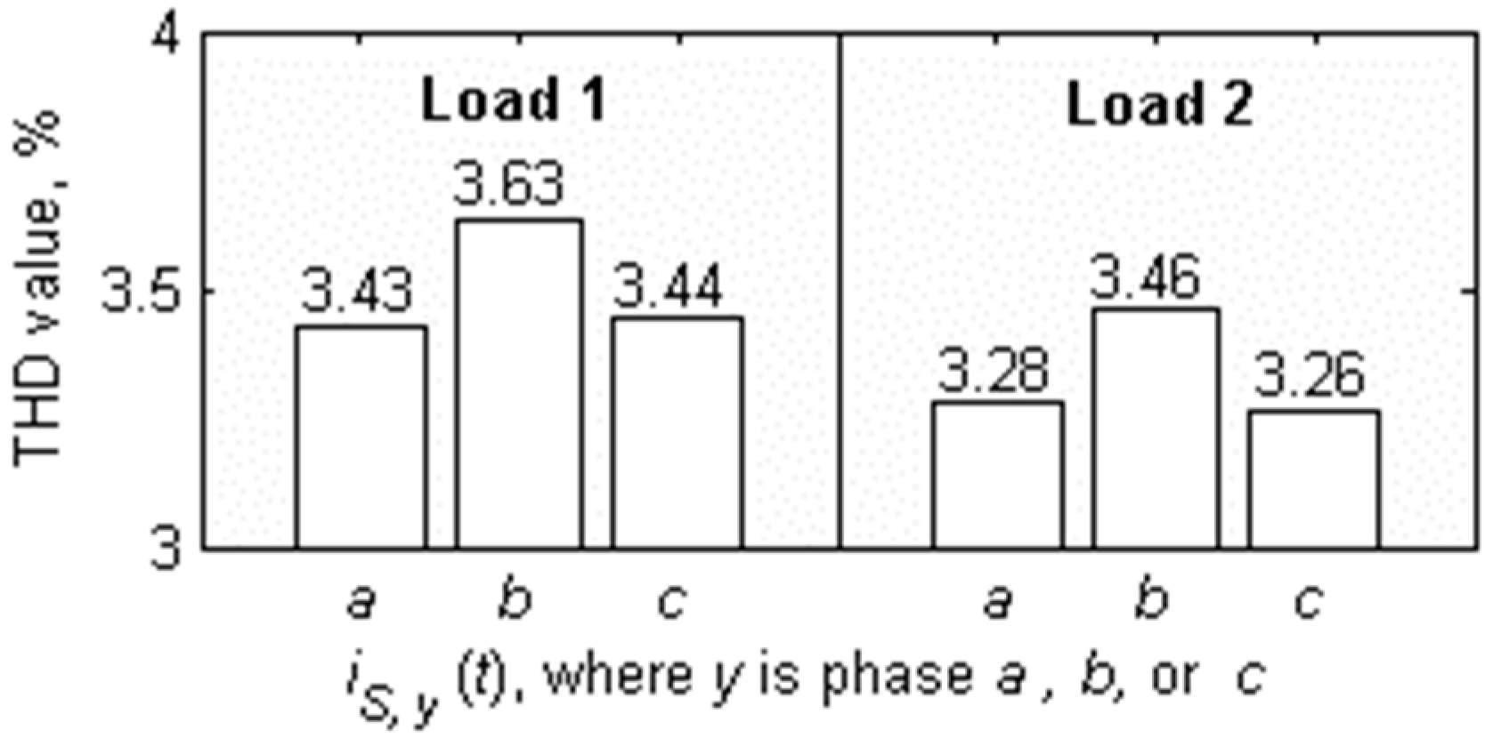
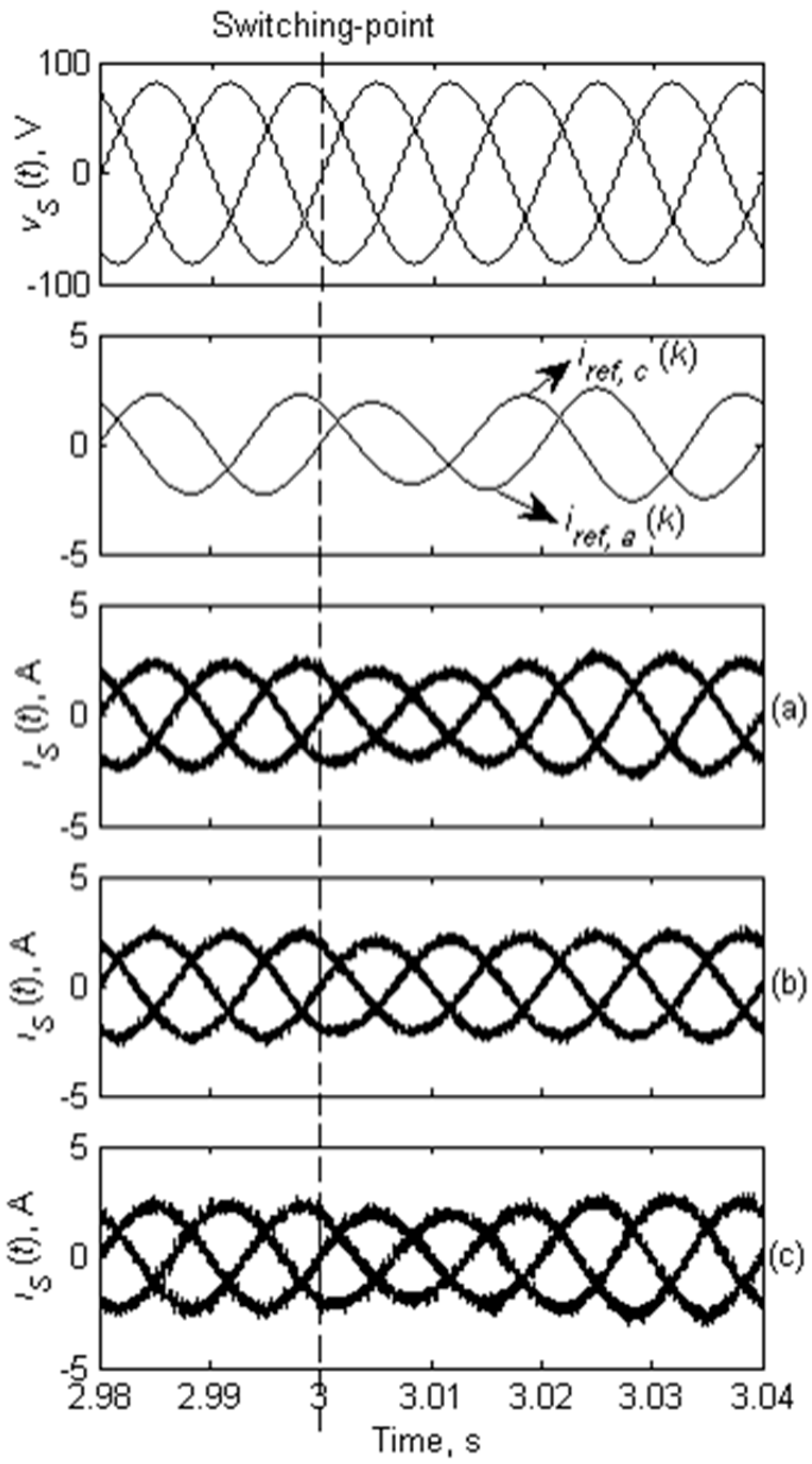
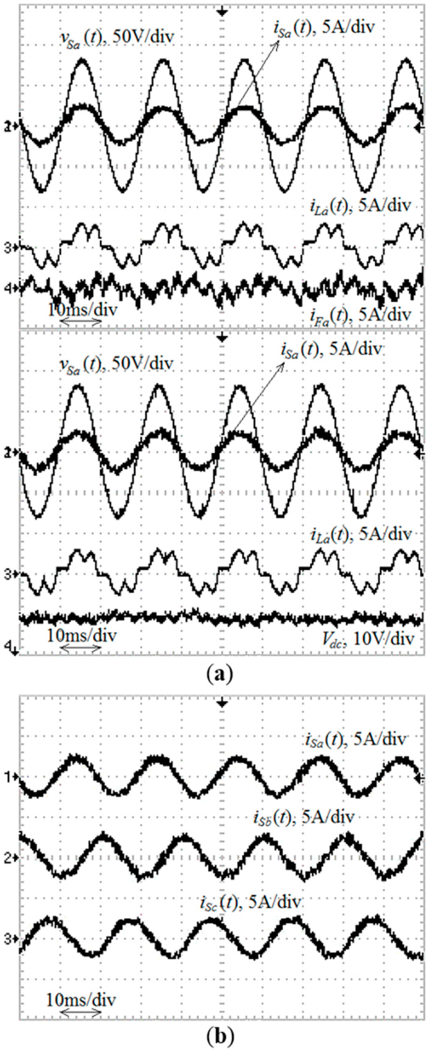
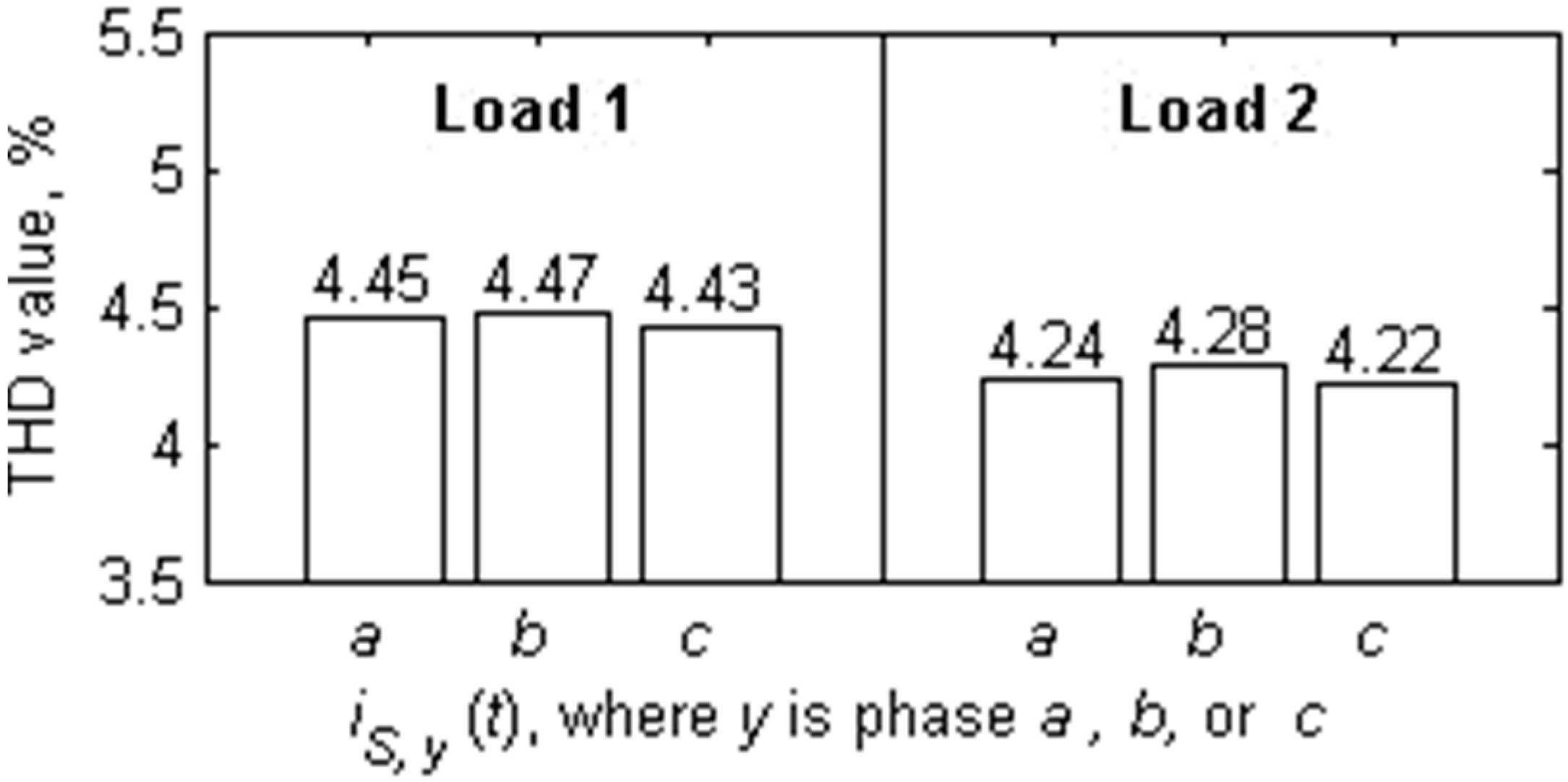
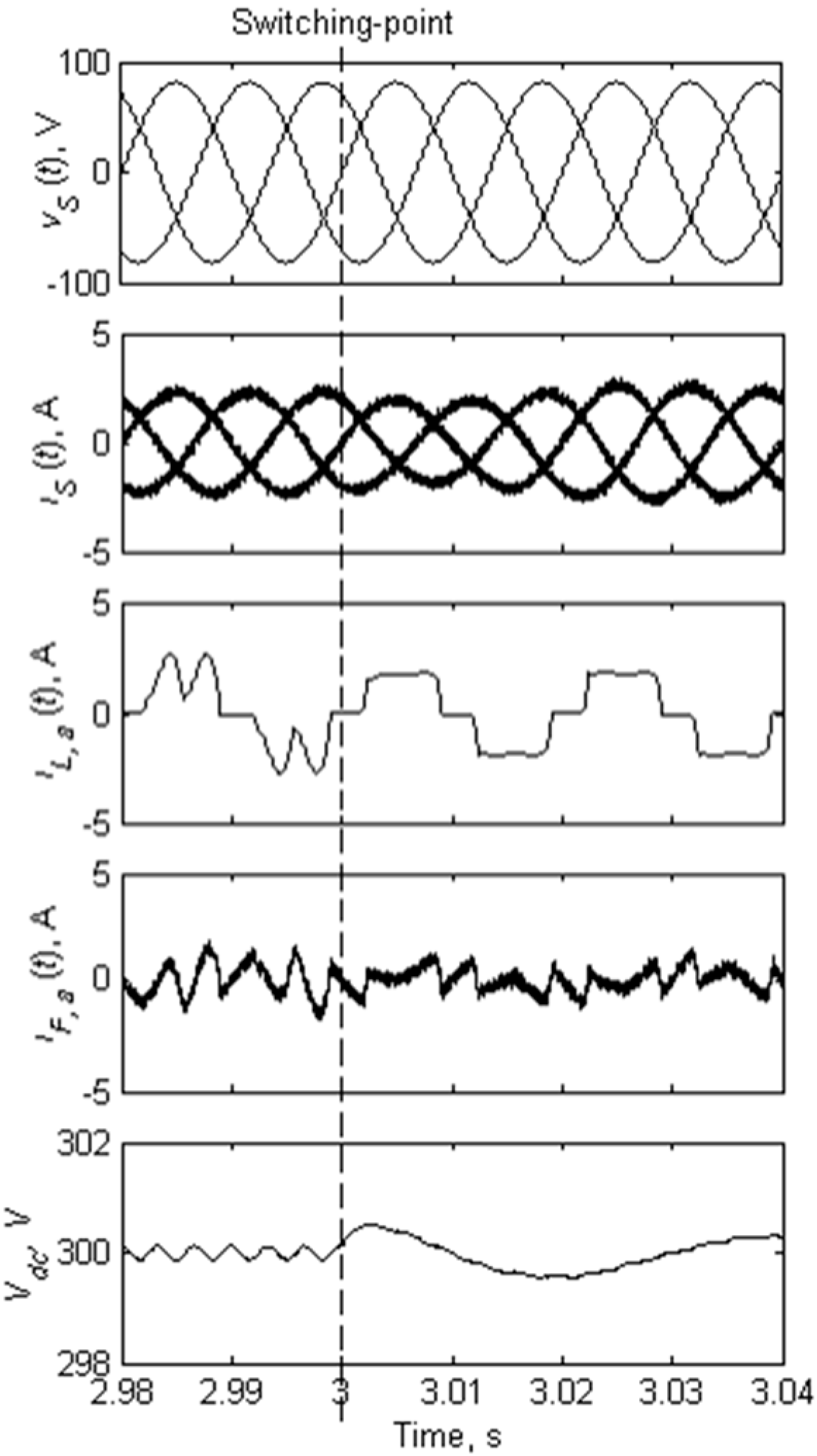
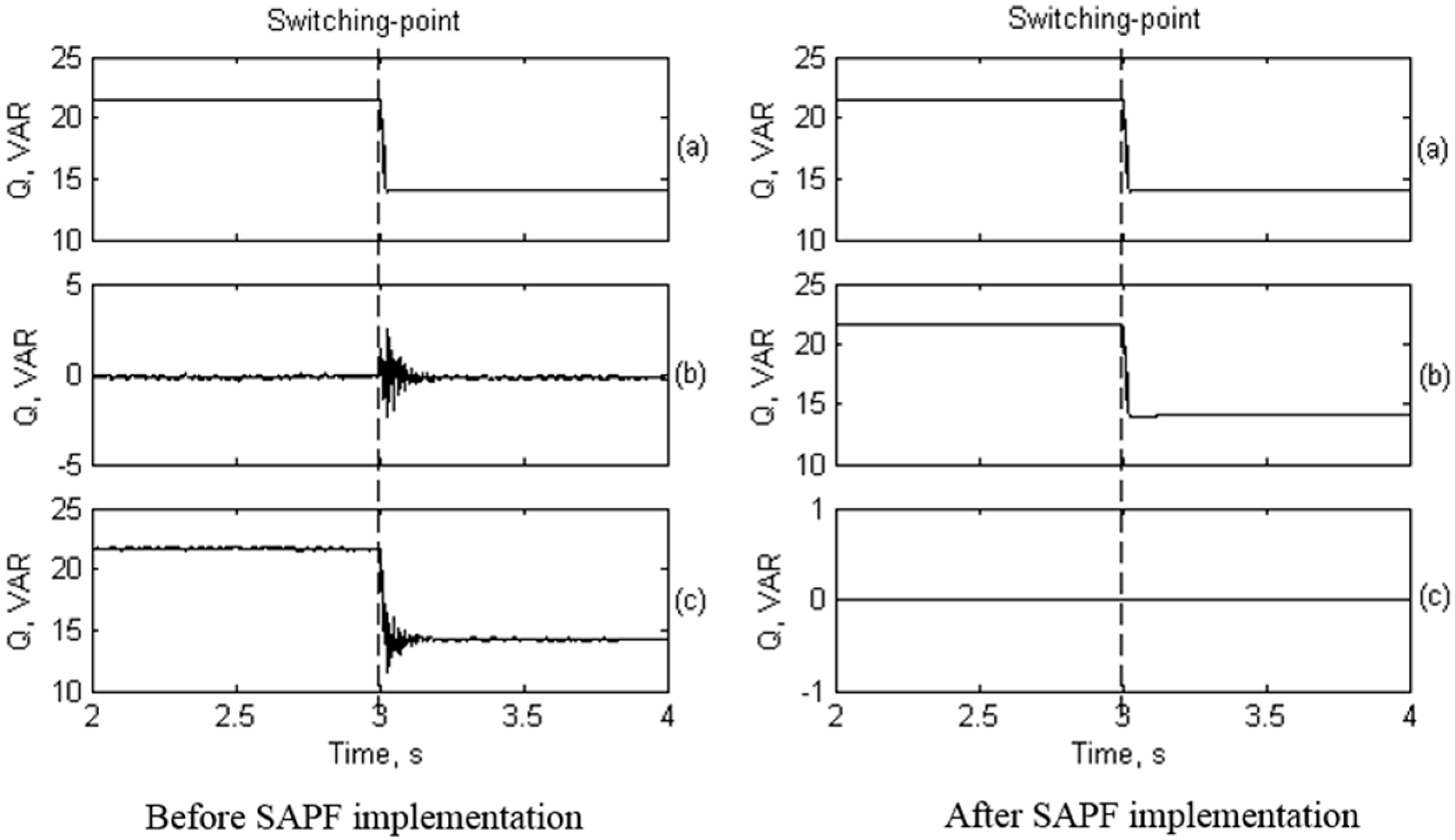
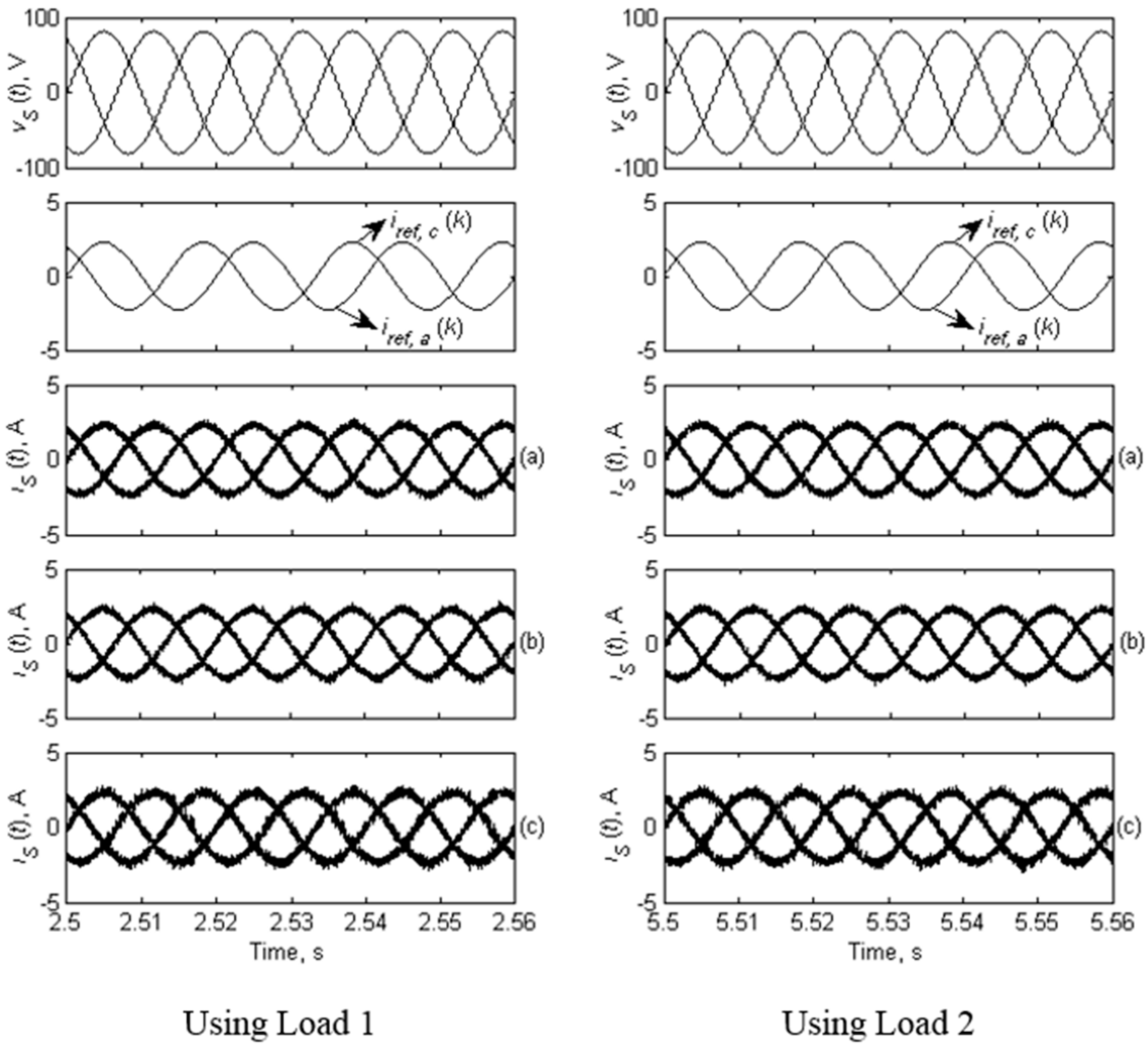
4.2. Harmonic Currents and Reactive Power Compensation
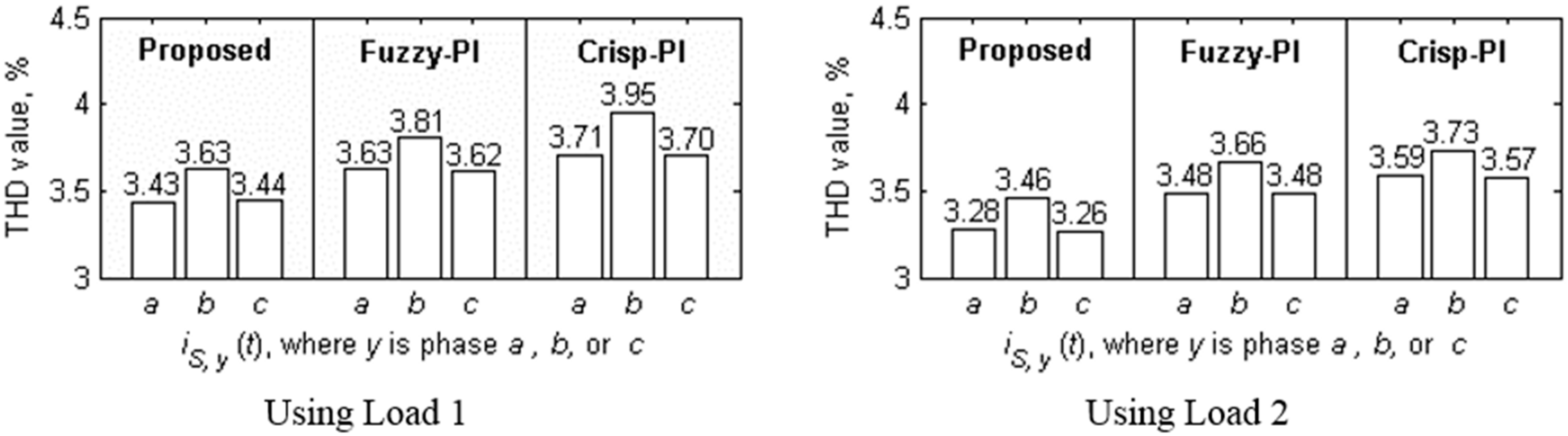
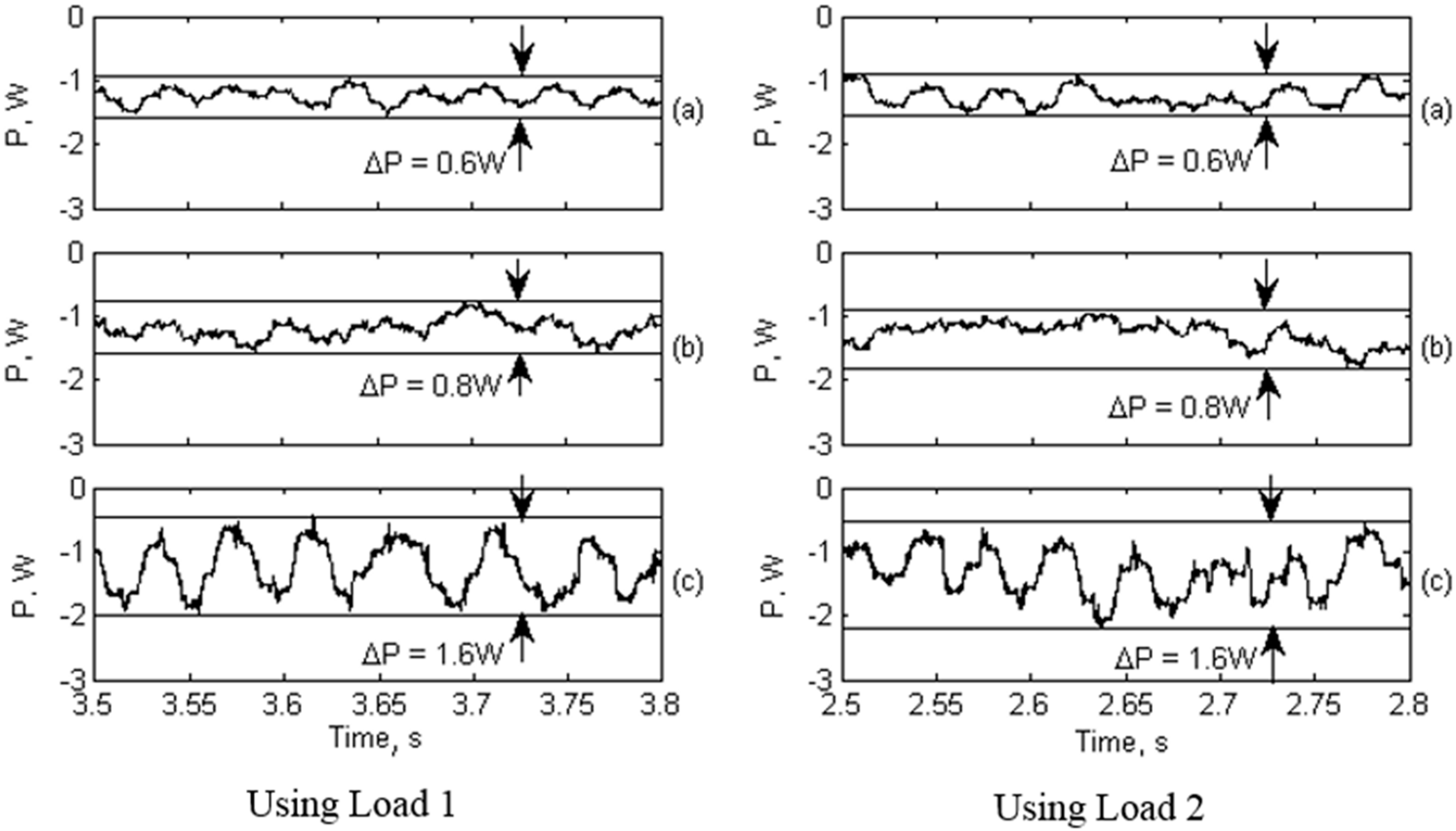
4.3. Comparison of Performance with Other Proportional-Integral Current Control Algorithms
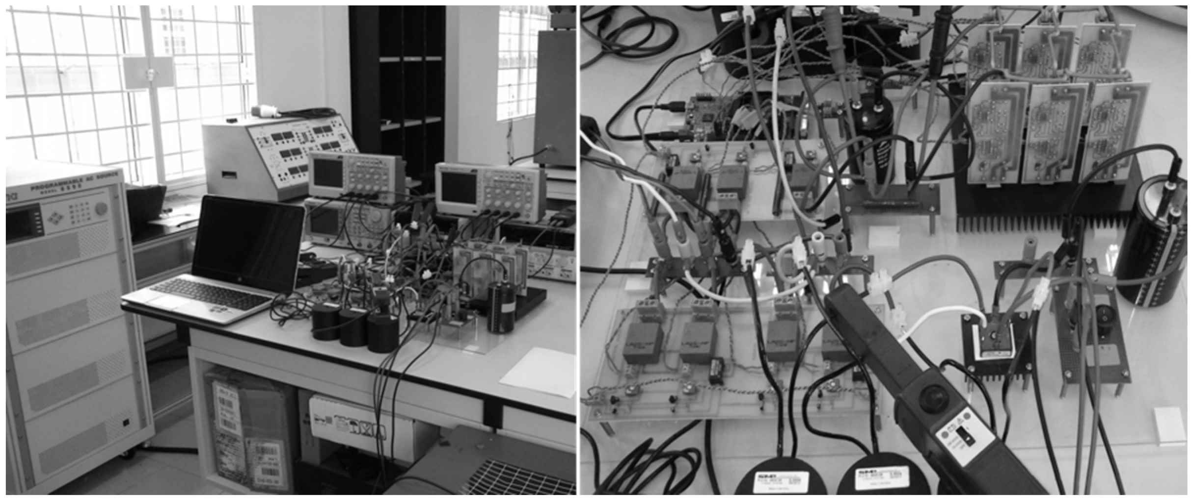
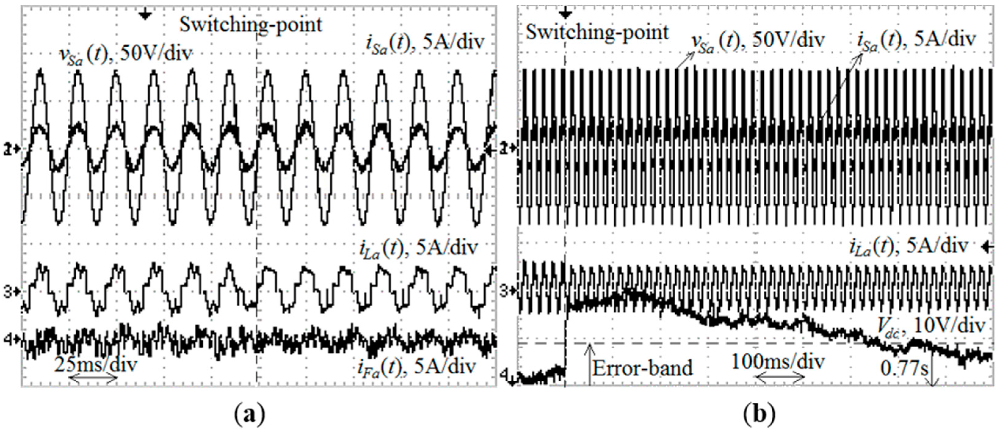
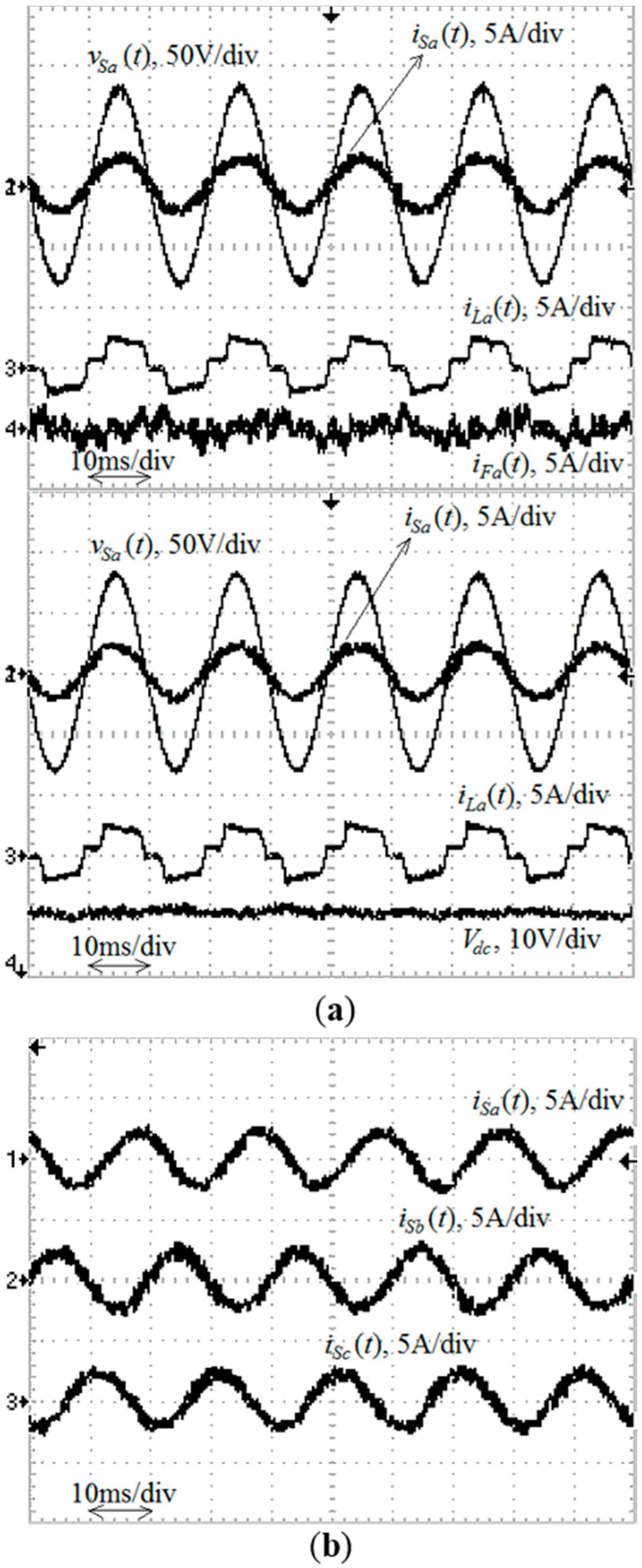
5. Experimental Work
6. Conclusions
Acknowledgments
Author Contributions
Conflicts of Interest
References
- Rashid, M.H. Power Electronics Handbook Devices, Circuits, and Applications, 3rd ed.; Elsevier: Oxford, UK, 2011; pp. 1–1193. [Google Scholar]
- Shahbaz, M. Active Harmonics Filtering for Distributed AC Systems. Master’s Thesis, Norwegian University of Science and Technology, Trondheim, Norway, 2012. [Google Scholar]
- Singh, B.; Al-Haddad, K.; Chandra, A. A review of active filters for power quality improvement. IEEE Trans. Ind. Electron. 1999, 46, 960–971. [Google Scholar] [CrossRef]
- Bouloumpasis, I.; Vovos, P.; Georgakas, K.; Vovos, N. Current harmonics compensation in microgrids exploiting the power electronics interfaces of renewable energy sources. Energies 2015, 8, 2295–2311. [Google Scholar] [CrossRef]
- Qasim, M.; Kanjiya, P.; Khadkikar, V. Artificial-neural-network-based phase-locking scheme for active power filters. IEEE Trans. Ind. Electron. 2014, 61, 3857–3866. [Google Scholar] [CrossRef]
- Kinhal, V.G.; Agarwal, P.; Gupta, H.O. Performance investigation of neural-network-based unified power-quality conditioner. IEEE Trans. Power Deliv. 2011, 26, 431–437. [Google Scholar] [CrossRef]
- Singh, B.; Verma, V.; Solanki, J. Neural network-based selective compensation of current quality problems in distribution system. IEEE Trans. Ind. Electron. 2007, 54, 53–60. [Google Scholar] [CrossRef]
- Bojoi, R.; Limongi, L.R.; Roiu, D.; Tenconi, A. Enhanced power quality control strategy for single-phase inverters in distributed generation systems. IEEE Trans. Power Electron. 2011, 26, 798–806. [Google Scholar] [CrossRef]
- Xin, T.; Tsang, K.M.; Chan, W.L. A power quality compensator with dg interface capability using repetitive control. IEEE Trans. Energy Convers. 2012, 27, 213–219. [Google Scholar]
- Ramos, G.A.; Costa-Castelló, R. Power factor correction and harmonic compensation using second-order odd-harmonic repetitive control. IET Control Theory Appl. 2012, 6, 1633–1644. [Google Scholar] [CrossRef]
- Hamad, M.S.; Masoud, M.I.; Williams, B.W.; Finney, S. Medium voltage 12-pulse converter: AC side compensation using a shunt active power filter in a novel front end transformer configuration. IET Power Electron. 2012, 5, 1315–1323. [Google Scholar] [CrossRef]
- Yaramasu, V.; Rivera, M.; Bin, W.; Rodriguez, J. Model Predictive Current Control of Two-Level Four-Leg Inverters-Part I: Concept, Algorithm, and Simulation Analysis. IEEE Trans. Power Electron. 2013, 28, 3459–3468. [Google Scholar] [CrossRef]
- Rivera, M.; Yaramasu, V.; Rodriguez, J.; Bin, W. Model predictive current control of two-level four-leg inverters-part ii: Experimental implementation and validation. IEEE Trans. Power Electron. 2013, 28, 3469–3478. [Google Scholar] [CrossRef]
- Matas, J.; de Vicuna, L.G.; Miret, J.; Guerrero, J.M.; Castilla, M. Feedback linearization of a single-phase active power filter via sliding mode control. IEEE Trans. Power Electron. 2008, 23, 116–125. [Google Scholar] [CrossRef]
- Djazia, K.; Krim, F.; Chaoui, A.; Sarra, M. Active power filtering using the ZDPC method under unbalanced and distorted grid voltage conditions. Energies 2015, 8, 1584–1605. [Google Scholar] [CrossRef]
- Chandra, A.; Singh, B.; Singh, B.N.; Al-Haddad, K. An improved control algorithm of shunt active filter for voltage regulation, harmonic elimination, power-factor correction, and balancing of nonlinear loads. IEEE Trans. Power Electron. 2000, 15, 495–507. [Google Scholar] [CrossRef]
- Rahmani, S.; Hamadi, A.; Al-Haddad, K.; Dessaint, L.A. A combination of shunt hybrid power filter and thyristor-controlled reactor for power quality. IEEE Trans. Ind. Electron. 2014, 61, 2152–2164. [Google Scholar] [CrossRef]
- Rahmani, B.; Li, W.; Liu, G. A wavelet-based unified power quality conditioner to eliminate wind turbine non-ideality consequences on grid-connected photovoltaic systems. Energies 2016, 9, 390. [Google Scholar] [CrossRef]
- Panda, A.K.; Mikkili, S. FLC based shunt active filter (p-q and id-iq) control strategies for mitigation of harmonics with different fuzzy mfs using matlab and real-time digital simulator. Int. J. Electr. Power Energy Syst. 2013, 47, 313–336. [Google Scholar] [CrossRef]
- Chang, G.W.; Shee, T.C. A novel reference compensation current strategy for shunt active power filter control. IEEE Trans. Power Deliv. 2004, 19, 1751–1758. [Google Scholar] [CrossRef]
- Vodyakho, O.; Mi, C.C. Three-Level inverter-based shunt active power filter in three-phase three-wire and four-wire systems. IEEE Trans. Power Electron. 2009, 24, 1350–1363. [Google Scholar] [CrossRef]
- Chen, Z.; Wang, Z.; Chen, M. Four hundred hertz shunt active power filter for aircraft power grids. IET Power Electron. 2014, 7, 316–324. [Google Scholar] [CrossRef]
- Xiao, Z.; Deng, X.; Yuan, R.; Guo, P.; Chen, Q. Shunt active power filter with enhanced dynamic performance using novel control strategy. IET Power Electron. 2014, 7, 3169–3181. [Google Scholar] [CrossRef]
- Odavic, M.; Biagini, V.; Zanchetta, P.; Sumner, M.; Degano, M. One-sample-period-ahead predictive current control for high-performance active shunt power filters. IET Power Electron. 2011, 4, 414–423. [Google Scholar] [CrossRef]
- Kumar, P.; Mahajan, A. Soft computing techniques for the control of an active power filter. IEEE Trans. Power Deliv. 2009, 24, 452–461. [Google Scholar] [CrossRef]
- Luo, A.; Shuai, Z.; Zhu, W.; Shen, Z.J. Combined system for harmonic suppression and reactive power compensation. IEEE Trans. Ind. Electron. 2009, 56, 418–428. [Google Scholar] [CrossRef]
- Suetake, M.; da Silva, I.N.; Goedtel, A. Embedded DSP-based compact fuzzy system and its application for induction-motor v/f speed control. IEEE Trans. Ind. Electron. 2011, 58, 750–760. [Google Scholar] [CrossRef]
- Kirawanich, P.; Oconnell, R.M. Fuzzy logic control of an active power line conditioner. IEEE Trans. Power Electron. 2004, 19, 1574–1585. [Google Scholar] [CrossRef]
- Rahman, N.F.A.; Radzi, M.A.M.; Soh, A.C.; Mariun, N.; Rahim, N.A. Dual function of unified adaptive linear neurons based fundamental component extraction algorithm for shunt active power filter operation. Int. Rev. Electr. Eng. 2015, 10, 544–552. [Google Scholar]
- Rahman, N.F.A.A.; Radzi, M.A.M.; Mariun, N.; Soh, A.C.; Rahim, N.A. Integration of dual intelligent algorithms in shunt active power filter. In Preceedings of the 2013 IEEE Conference on Clean Energy and Technology, Langkawi, Malaysia, 18–20 November 2013.
- Suresh, Y.; Panda, A.K.; Suresh, M. Real-time implementation of adaptive fuzzy hysteresis-band current control technique for shunt active power filter. IET Power Electron. 2012, 5, 1188–1195. [Google Scholar] [CrossRef]
- Jantzen, J. Foundation of Fuzzy Control, 1st ed.; Wiley: London, UK, 2007; pp. 1–57. [Google Scholar]
- Bhattacharya, A.; Chakraborty, C. A shunt active power filter with enhanced performance using ann-based predictive and adaptive controllers. IEEE Trans. Ind. Electron. 2011, 58, 421–428. [Google Scholar] [CrossRef]
- Borisov, K.; Ginn, H.L.; Trzynadlowski, A.M. Attenuation of electromagnetic interference in a shunt active power filter. IEEE Trans. Power Electron. 2007, 22, 1912–1918. [Google Scholar] [CrossRef]


| NB | NB |
| NM | NM |
| NS | NS |
| ZE | ZE |
| PS | PS |
| PM | PM |
| PB | PB |
| Description | Value | |
|---|---|---|
| 3-phase line-to-line voltage supply | 100 V | |
| Line inductor | 5 mH | |
| Filter inductor | 5 mH | |
| Dc-link capacitor | 2200 μF | |
| Dc-link voltage reference | 300 V | |
| Load 1: | Resistor Capacitor | 43 Ω and 63 Ω 470 μF |
| Load 2: | Resistor Inductor | 43 Ω and 63 Ω 80 mH |
© 2016 by the authors; licensee MDPI, Basel, Switzerland. This article is an open access article distributed under the terms and conditions of the Creative Commons Attribution (CC-BY) license (http://creativecommons.org/licenses/by/4.0/).
Share and Cite
Abdul Rahman, N.F.; Mohd Radzi, M.A.; Che Soh, A.; Mariun, N.; Abd Rahim, N. Adaptive Hybrid Fuzzy-Proportional Plus Crisp-Integral Current Control Algorithm for Shunt Active Power Filter Operation. Energies 2016, 9, 737. https://doi.org/10.3390/en9090737
Abdul Rahman NF, Mohd Radzi MA, Che Soh A, Mariun N, Abd Rahim N. Adaptive Hybrid Fuzzy-Proportional Plus Crisp-Integral Current Control Algorithm for Shunt Active Power Filter Operation. Energies. 2016; 9(9):737. https://doi.org/10.3390/en9090737
Chicago/Turabian StyleAbdul Rahman, Nor Farahaida, Mohd Amran Mohd Radzi, Azura Che Soh, Norman Mariun, and Nasrudin Abd Rahim. 2016. "Adaptive Hybrid Fuzzy-Proportional Plus Crisp-Integral Current Control Algorithm for Shunt Active Power Filter Operation" Energies 9, no. 9: 737. https://doi.org/10.3390/en9090737