Does Your Domestic Photovoltaic Energy System Survive Grid Outages?

Abstract

Domestic renewable energy systems, including photovoltaic energy generation, as well as local storage, are becoming increasingly popular and economically feasible, but do come with a wide range of options. Hence, it can be difficult to match their specification to specific customer’s needs. Next to the usage-specific demand profiles and location-specific production profiles, local energy storage through the use of batteries is becoming increasingly important, since it allows one to balance variations in production and demand, either locally or via the grid. Moreover, local storage can also help to ensure a continuous energy supply in the presence of grid outages, at least for a while. Hybrid Petri net (HPN) models allow one to analyze the effect of different battery management strategies on the continuity of such energy systems in the case of grid outages. The current paper focuses on one of these strategies, the so-called smart strategy, that reserves a certain percentage of the battery capacity to be only used in case of grid outages. Additionally, we introduce a new strategy that makes better use of the reserved backup capacity, by reducing the demand in the presence of a grid outage through a prioritization mechanism. This new strategy, called power-save, only allows the essential (high-priority) demand to draw from the battery during power outages. We show that this new strategy outperforms previously-proposed strategies through a careful analysis of a number of scenarios and for a selection of survivability measures, such as minimum survivability per day, number of survivable hours per day, minimum survivability per year and various survivability quantiles.

1. Introduction

Over the last decade, we have witnessed an enormous increase in local (distributed) energy generation, e.g., through photovoltaic panels. Recent changes in national subsidy schemes, as for example in Germany, also lead to an increased interest in local battery storage systems, as this appears economically more attractive. When managed in a grid-convenient way, recent research [1,2] suggests that local energy storage may lead to a more balanced grid, but can also be used to increase the energy independence in the case of grid outages. While the importance of the latter may not be immediately obvious, related work states that due to the variability in power production introduced by decentralized renewable power generation, the number of grid failures is expected to increase up to 60% until 2020 [3]. Furthermore, in many countries, grid outages occur more regularly than one is used to in countries like Germany or the Netherlands (where the authors reside). In [4], it is suggested that the combined use of photovoltaic generation and local (community) storage is an important way to go for increasing power delivery resilience; we exactly investigate that in this paper.

Domestic renewable energy systems are small-scale energy installations that may be integrated into a building already at design time or later as an add-on. Most of the time, they include a set of photovoltaic (PV) panels, whose orientation and tilt will determine the total production that can be achieved. A battery that is added to the system for local storage is able to balance small-scale variations between production and demand. The capacity of the battery, as well as the battery management strategy have a large impact on the available energy throughout a day. Such a system can be installed as a stand-alone, i.e., not connected to the grid at all, or as an online system and then needs to take into account the grid-connection requirements from the local provider. Safety equipment and net-metering needs to be added to the system in such cases in order to ensure safe operation and correct accounting.

Next to renewable energy systems, plenty of other extensions are possible in the context of smart homes and home automation, including heat pumps, automated temperature regulation, CCHP (combined chilling-heating-power generators) or charging stations for electric vehicles [5]. Smart appliances and smart plugs [6] can control, e.g., white goods, whenever solar energy is available, hence, can be used for load balancing on a distributed scale. Clearly, this requires reliable communication protocols [7,8] that are able to control the interplay between the different modules; the project e-balance develops and evaluates such communication protocols [9].

The focus of this paper is, however, on domestic energy systems with just local generation and local storage. We do, however, assume the availability of smart devices/smart plugs that allow one to reduce the demand in the presence of a power outage. For home owners or installation companies, it can be difficult to estimate which battery size is needed to match their specific needs, especially when different battery management strategies are available. This paper provides the means to oversee the effect of different storage capacities on the continuous availability of the power supply. To better take into account the variability of production and demand for different types of households and solar installations, we have used the Artificial Load Profile Generator (ALPG) [10] to generate appropriate production and demand profiles for a full year. Using these, we then compute the probability that the effective energy supply is not interrupted by a grid outage (the so-called survivability probability [11,12,13]; see also Section 5). Note that this probability not only depends on the demand and production profile, but also on the capacity and state-of-charge of the battery at the moment the outage occurs, as well as on the outage duration (distribution) and the employed battery management strategy.

By introducing stochastic durations for grid outages, we used previously developed algorithms [14] to analyze the impact of such outages for a whole range of battery sizes and by taking every hour as a potential starting point for a grid failure. Previously, we mainly used the so-called smart strategy, which reserves a certain percentage of the battery capacity to be used only in the case of a power outage. This paper introduces a new battery management strategy that attempts to make better use of the reserved backup capacity, by also reducing the demand in the presence of power outages. This new strategy, called power-save, only allows the essential demand to be drawn from the battery during a power outage.

The survivability of a solar energy system with a local storage in the presence of stochastic power outages has also been investigated in [15]. The trade-off in terms of cost between a flexible battery use and reserving a certain amount of battery capacity as backup is investigated in [16]. Both works combine deterministic demand [17] and production profiles [18] for exemplary days in different seasons, with an abstract battery model for a single house. The current paper extends the work of [15] and [16] in the following ways:

• The new battery management strategy power-save is included in the model, which reduces the demand in the case of a power outage.
• To better reflect the variability of production and demand, we analyze the survivability of the energy system for every day of a complete year, using synthesized profiles obtained from the tool ALPG [10] for a particular type of household.
• We are able to show that for medium-sized batteries (between 2.5 kWh and 3.5 kWh), the power-save strategy outperforms the smart strategy considerably, i.e., it almost doubles the minimum survivability that can be achieved.

The paper is further organized as follows. Section 2 discusses related work on smart grids and domestic smart energy systems. Section 3 introduces the scenario for a domestic smart energy system that will be used throughout the rest of the paper. Section 4 explains the hybrid Petri net model for the presented scenario, and Section 5 introduces the parameter choices and the measures of interest. Section 6 presents and discusses the computed survivability results for both battery management strategies. Section 7 concludes the paper.

2. Related Work

Next to our own previous work on this topic (cf. [15,16]), there is much related work on the topic at large, however not much that addresses the effect of grid outages on the system survivability. We discuss important approaches below. Furthermore, the general topic of (network) survivability evaluation has been studied in detail in the past two decades; please refer to [11,12,13] and the references therein.

Related work on smart grids mainly models the stability of the grid in the presence of renewable generation [19,20], focuses on optimization [21,22] or presents relatively simple Petri net models for dependability assessment [23]. Economical aspects are discussed in [24,25]; the authors conclude that from a purely economical viewpoint, PV-battery systems are not interesting, yet. However, in these studies, resiliency and survivability are not addressed.

While both, grid stability and economical aspects are clearly important, the occurrence of random grid outages makes energy resilience in a domestic environment an important topic; see also [4]. Related work specifically on grid resilience primarily focuses on the resilience of the high- and medium-voltage grid and is studied in terms of the (expected) energy not supplied per unit of time (see, e.g., [26,27]), often computed using time-scale decomposition; we refer to [13] for a recent survey. In contrast, we address the resilience of the energy delivery (in terms of surviving grid outages) from the perspective of an end-customer.

The use of local storage is often considered for grid balancing and peak shaving [28,29,30,31]. Related work on energy management strategies mainly focuses on optimization, e.g., through evolutionary algorithms [32], mixed-integer linear programming [33] or model predictive control [30]. Adaptive strategies take into account the weather prediction as in [34,35] to achieve a robust management strategy. Since the main objective for these works is grid balancing, they mostly evaluate the interests of the grid operator.

Furthermore, the work by German et al. [36,37] addresses the analysis of smart energy systems with locally-generated electricity and local or distributed storage. However, it does so by only using simulation and does not address the notion of energy resilience under grid outages.

In contrast, this and our recent work [15,16] focus on the interest of the end-user in the presence of power outages. We consider the grid simply as a source of energy with possible interruptions. The models we use are truly stochastic hybrid models, in that they combine deterministic events with probabilistic events on a mixed discrete/continuous state space. This combination allows us to investigate the consequences of grid failures with random durations on the continuous energy supply of the house. This has not been done before. Note that the solution we propose does have a cost, because we will not always use locally-generated (and stored) energy, even though it is in principle available, simply because we reserve it for backup purposes. The current work can be extended to also take costs into account, in a similar way as has been done in [16].

3. Domestic Smart Energy System

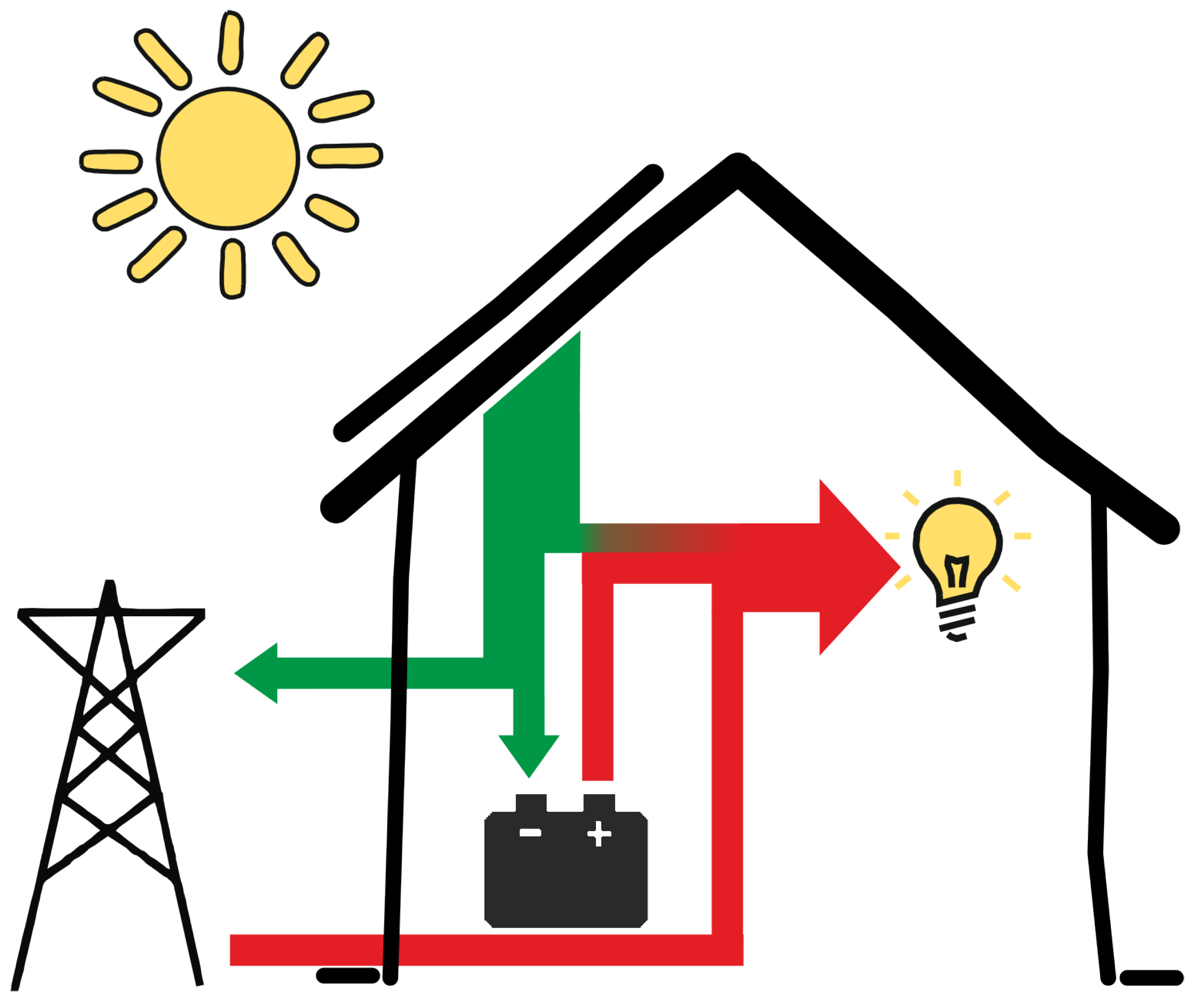
We consider a domestic smart energy system (“a house”) that is equipped with a solar energy system and local storage in the form of a battery. Figure 1 gives a schematic overview of the energy flows within such a house. The produced energy can be supplied directly to the demand, if any; it can be stored in the battery or fed back into the grid. The electricity demand is supplied by the local production, the battery or the grid. An energy management system decides when to use which energy source. In the following subsections, we will discuss demand and production, local storage and the energy management system, respectively.

3.1. Demand and Production

We consider the production and demand within the house for a period of one year. We use the Artificial Load Profile Generator (ALPG) developed by Hoogsteen et al. [10] to generate the demand and production profiles. The ALPG tool has been developed to synthesize power profiles for different household types for the analysis of demand-side management algorithms. The generated demand profiles consist of several static categories: standby, electronics, lighting, fridge, inductive and other. Additionally, the tool includes flexible loads, such as a smart washing machine, dishwasher and electrical vehicles. The loads for the washing machine and dishwasher consist of the power profile of a single cycle of the machine and the time interval within which such a cycle must run.

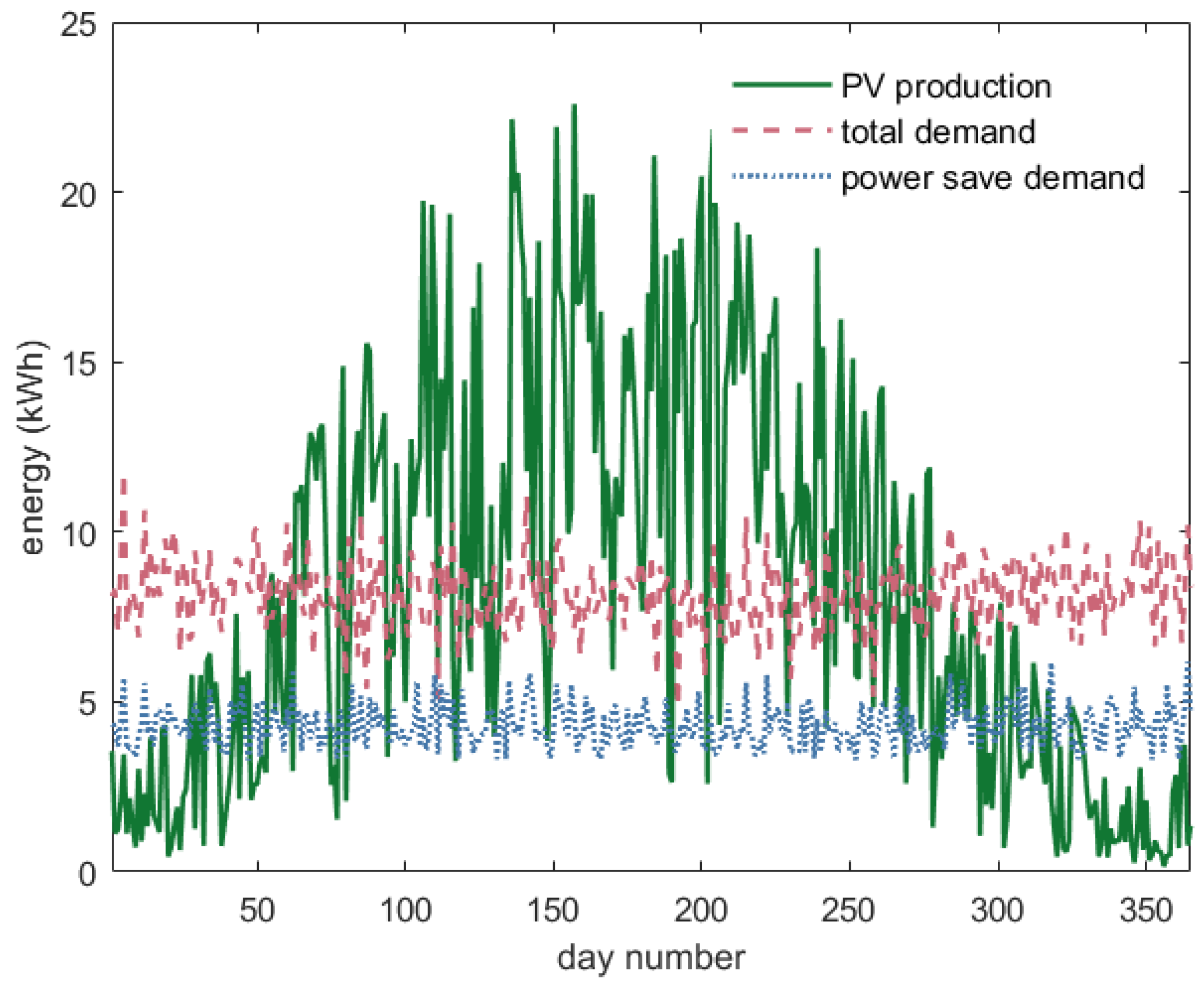
We generated a demand profile for a so-called FamilyDualWorker household, with a smart washing machine and dishwasher. Since we do not aim at scheduling flexible loads, we fix the starting time of smart appliances always to the earliest possible time point. From the ALPG tool, we obtain a minute-based demand profile with a total yearly demand of 2983 kWh. The per minute demand values are aggregated to hourly demand values, which are used in our model.

In case of a grid failure, part of the demand could be switched off to save energy, either by a home automation system or an energy-aware inhabitant of the house. We assume that the load categories electronics, lighting and inductive can be turned off, as well as the flexible loads of the washing machine and dishwasher. The reduced, i.e., the power-save demand is roughly half of the full demand, at 1418 kWh per year.

The production profile computed with ALPG is based on weather data supplied by the Royal Netherlands Meteorological Institute (KNMI) [38] of the weather station Twenthe for the year 2014. The PV panels are set to face south, with a tilt of 35 degrees. The ALPG tool provides the energy production per hour. The obtained profile is scaled to a yearly production of approximately 3000 kWh to (closely) match the yearly demand. This would correspond to a PV system of approximately 3.3 kWh.

Figure 2 shows the daily production, total demand and power-save demand, for the modeled household. Day 1 corresponds to 1 January, and Day 365 corresponds to 31 December.

3.2. Local Storage

Within the house, the installed battery has two functions. First, the battery can be used to increase the amount of locally-produced energy that is also used locally (the so-called self-use). When the production is higher than the demand, part of the generated electricity can be stored temporarily in the battery, to be used later when the production is lower than the demand. In this way, the impact of the household on the grid is reduced. Furthermore, such an approach might be economically more attractive, as selling energy to the grid typically goes at lower prices per kWh than buying from the grid. The second function of the battery is to provide backup energy in the case of grid outages.

In the model, we only consider the so-called usable capacity of the battery. In practice, the battery will never be fully discharged in order to extend the cycle-life, i.e., the number of charge-discharge cycles until the battery is depleted. Commercial systems, such as Nedap’s PowerRouter [39], use lead-acid batteries with a usable capacity of 50% of the nominal capacity or lithium-ion batteries with a usable capacity of 70 to 80%. Note that the present study only considers the usable capacity of a battery; hence, this can be used for different kinds of battery storage. Since the battery is only partially discharged, the non-linear properties, such as the rate capacity and recovery effect [40], have a smaller impact. Therefore, we can model the battery as an ideal energy storage unit, without introducing large errors. We also do not consider the aging effects of the battery.

Note that a battery cannot be charged and discharged at the same time; hence, it is not feasible to store solar energy in the battery and power the house from the same battery at the same time. Hence, in practice, if the production is larger than the demand, the house is directly powered from the solar panels, and only the excess energy is stored in the battery. Please note that the presented model abstracts such technicalities and only considers the net sum of the energy flows.

3.3. Energy Management Strategies

In order to control the use of solar power and to decide in the absence of solar power whether the house has to be powered from the battery or from the grid, battery management strategies are needed. This paper focuses on the customer viewpoint and considers two strategies that support the survivability of a house with a renewable energy system.

Earlier work (cf. [15]) also considered the so-called greedy and conservative strategies: greedy always depletes the battery completely before drawing from the power grid and has been shown to lead to a very low survivability. In contrast, the conservative strategy also draws from the grid to recharge the battery if it has been discharged too much. Since this leads to very many state changes between ‘charging’ and ‘discharging’, which is not beneficial for the available capacity of the battery, this strategy is not recommended, nor further considered here.

The two strategies used in this paper are the smart strategy, as proposed in [15] and the (new) power-save strategy. The first uses the local production mainly to supply the local demand. When the production is higher than the demand, the excess energy is stored in the battery. Only when the battery is full is the local production fed to the grid. Reversely, when the demand is larger than the production, first the battery is used to supply the shortage in production. However, the battery is not fully discharged. The energy management system always reserves a certain percentage of the overall capacity, which may only be used in the case of power outages.

The power-save strategy works similar to the smart strategy when the grid is operational, thus reserving part of the battery capacity as backup. Only under grid outages does the strategy behave differently: in such cases, a predetermined part of the demand will be switched off. In this way, the demand is reduced to the level of the power-save demand, as shown in Figure 2. The reduced demand will clearly increase the probability that the house can survive a grid outage.

4. Hybrid Petri Net Model for a Domestic Smart Energy System

We enhance the hybrid Petri net model as presented in [15,16] by including the new battery management strategy power-save. We also adapt the demand and the production part of the model to cover longer time periods, instead of just single days.

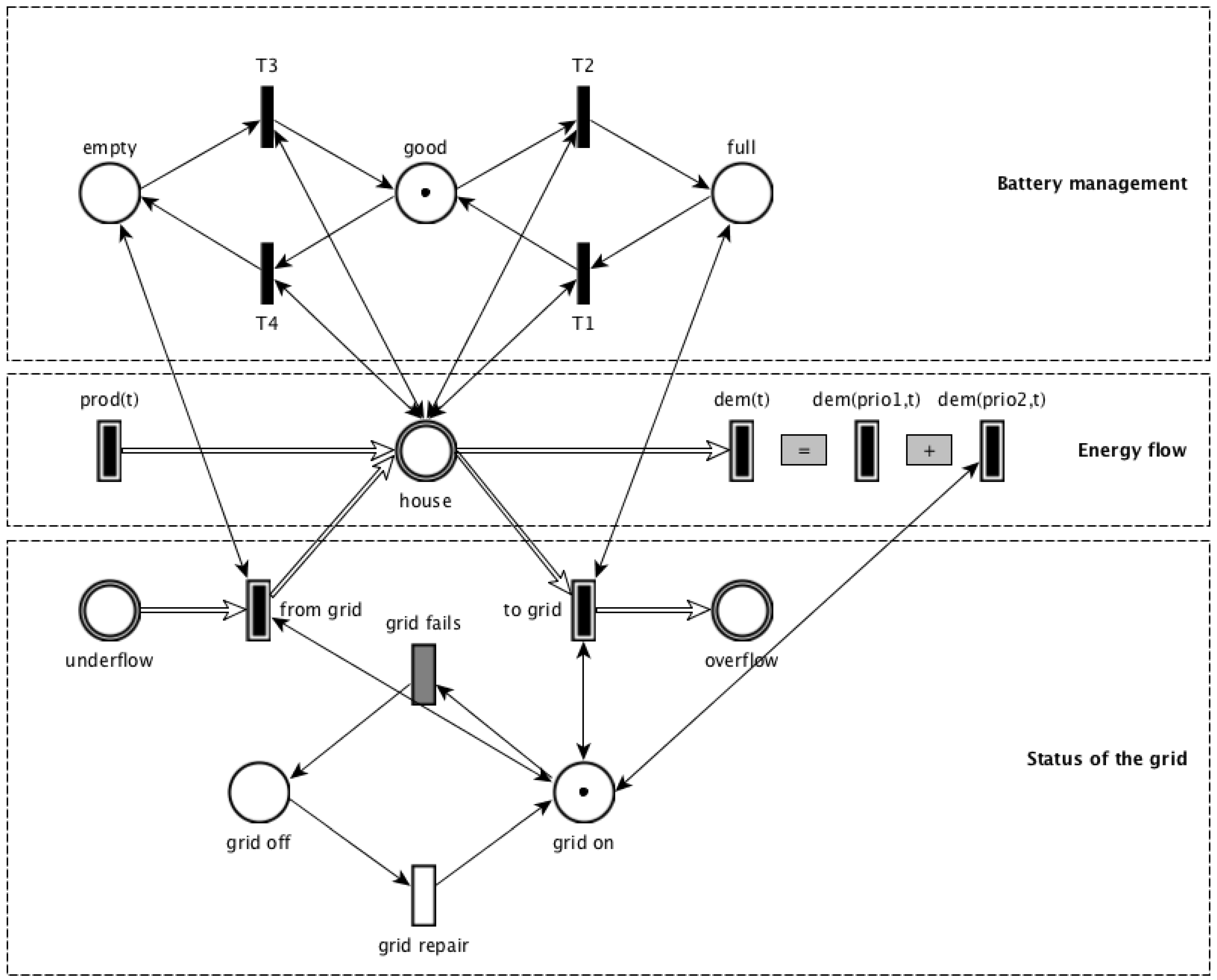
The model can be analyzed with existing techniques for hybrid Petri nets that allow for one stochastic variable in the model. This stochastic variable is used to describe the time that is needed for the grid to recover to an operational state again after the occurrence of an outage. In the following, we will briefly recall the main parts of the model; for details, we refer to [15]. Figure 3 shows an abstraction of the hybrid Petri net (HPN) model; it consists of three parts (from top to bottom): (i) the battery management system; (ii) the model of the battery together with production and demand; and (iii) the model for the status of the grid.

The battery is modeled as a continuous place with overall capacity B. Its current state (of charge) changes, with the time-dependent production $prod\left(t\right)$ and demand $dem\left(t\right)$, which represent the deterministic production and demand profiles during the day. When the local generation exceeds the demand and the storage capacity, the surplus is fed into the grid; similarly, energy is taken from the grid into the house when there is not enough local energy available. A bidirectional continuous arc represents the interaction between the battery and the grid. However, this interaction is only possible when the grid is operational. When the grid fails (modeled by the deterministic transition ‘grid fails’ at time a), the token is moved to place ‘grid off’, and the house is practically isolated from the grid. This allows us to study the impact of different time points of the grid failure occurrence. The grid returns from its failure, i.e., the outage ends, according to a stochastic repair time distribution that can be chosen freely.

The battery management system controls the flow of power between the local generation, the battery, the house and the grid, depending on the battery management strategy. The model distinguishes between three states of the battery; it can either be full, good or empty. In state empty, the battery cannot be discharged, although there might still be energy in it, which is, however, reserved as backup in case of grid failures. The transitions $T_i$ for $i\in \{1,2,3,4\}$ coordinate the change of state via test arcs that enable the firing of transition $T_i$ according to the available capacity of the battery. Transitions $T_1$ and $T_2$ are enabled if the state of charge of the battery equals the total battery capacity and a token is in place full and good, respectively. Transitions $T_3$ and $T_4$ are enabled if the state of charge equals the pre-defined backup level, e.g., $20\%$ or $30\%$ of the total battery capacity, and a token is available in place empty and good, respectively.

The newly-added battery management strategy, which turns off part of the demand when the grid fails, is realized through guard arcs between the low-priority demand and the place, which represents the grid working properly. This results in the high-priority demand being always served from the battery (if still possible) and the low priority demand only being served when the grid is available. This is illustrated on the right part of the figure, in which the actual demand at time t, i.e., $dem\left(t\right)$, equals the demand with priority 1 at time t, i.e., $dem(prio1,t)$, plus the demand with priority 2 at time t, i.e., $dem(prio2,t)$, if and only if the grid is working.

5. Case Study: Set-Up and Measures of Interest

We use the HPN model presented above to compute the survivability of the solar energy system for a certain set-up. While Section 5.1 repeats the main measure of survivability, Section 5.2 defines the notion of minimum survivability over a longer time period. Section 5.3 discusses parameter choices for the battery and the battery management strategies, as well as the initial setting of the presented case study.

5.1. Survivability

The main measure of interest in this paper is the probability to survive a grid outage, the so-called survivability, which is specified in the following for so-called given the occurrence of disaster (GOOD) models [13], where a failure (the power outage) is assumed to occur at a certain time a, specified in Stochastic Time Logic (STL) [14]:

$$\mathtt{survivability}=\mathtt{battery\_up}{\mathcal{U}}^{[\mathtt{a},\mathtt{a}+\mathtt{t}]}\mathtt{grid\_on}.$$

(1)

The above logical STL expression specifies that power is available from the battery continuously until the grid is repaired within t time units, after a grid outage occurring at time point a. For finite values of t, efficient algorithms for validating such formulae are available [14,41].

The time of failure a is a parameter of the model, in order to consider the impact of different failure time points during the day. Although power outage times are monitored and reported by the Council of European Energy Regulators (CEER) [42], providing numbers on average outage times, we did not manage to obtain information on outage duration distributions, even though we contacted several grid operators directly about this. It is stated in [43] that the number and duration of interruptions in European networks is generally low, ranging from about 15 min to 400 min a year. In the following, we assume that the repair time of the grid is distributed according to a folded normal distribution with parameters $\mu =0.5$ and $\sigma =1$. The time bound t (in the survivability expression) is chosen to be 5 h, since for the used repair duration distribution, the probability that the grid is not repaired within 5 h is smaller than ${10}^{-10}$.

5.2. Minimum Survivability per Day

As in [16], we compute the minimum survivability over longer periods of time. This is done by simply taking the minimum value of all computed survivability for the considered time period. This can be done, e.g., for a single day or a full year and allows us to reason about which setting has to be chosen to ensure a minimal required survivability.

5.3. Set-Up

We analyze the two strategies smart and power-save with respect to the resulting survivability for a backup capacity of 20% and 30% of the overall battery capacity of 3 kWh. To evaluate the system for a full year with changing demand and production patterns per day, we split the year into segments of several days and assume each hour as a possible outage occurrence (this corresponds to the choices for parameter a).

Note that the underlying state-space of the HPN models incorporates their evolution over time. Hence, evaluating a model for a longer time period results in a larger state-space. When combining multiple failure times in one model, the model needs to expand at least to the maximum failure time plus the specified time for recovery t (cf. Equation (1)). Furthermore, the size of the underlying state-space depends on the number of state changes that may occur. This results in differently-sized models for the different strategies. For the smart strategy, we are able to deal with models of eight days, and for the power-save strategy, we are only able to evaluate models of three days. This is due to the added number of state changes that occur when part of the demand is switched off in the case of a power outage.

For each generated model, the hourly parameters for demand and production are automatically loaded from the ALPG tool and entered into the HPN model to instrument the transitions $dem\left(t\right)$ and $prod\left(t\right)$. Furthermore, we initialize the state of charge of the battery with the correct value assuming that no grid failure has occurred recently. These initial values are obtained by executing the model without a grid failure for a year.

6. Results and Discussion

We present the results for two different battery management strategies and different backup levels. Section 6.1 presents and discusses the minimum survivability for the smart strategy, and Section 6.2 does the same for the power-save strategy. Section 6.3 analyzes the minimum survivability for a full year for both strategies as a function of the battery capacity. Note that all results are computed using the load and demand profile shown in Figure 2.

6.1. Smart Strategy with Two Different Backup Capacities

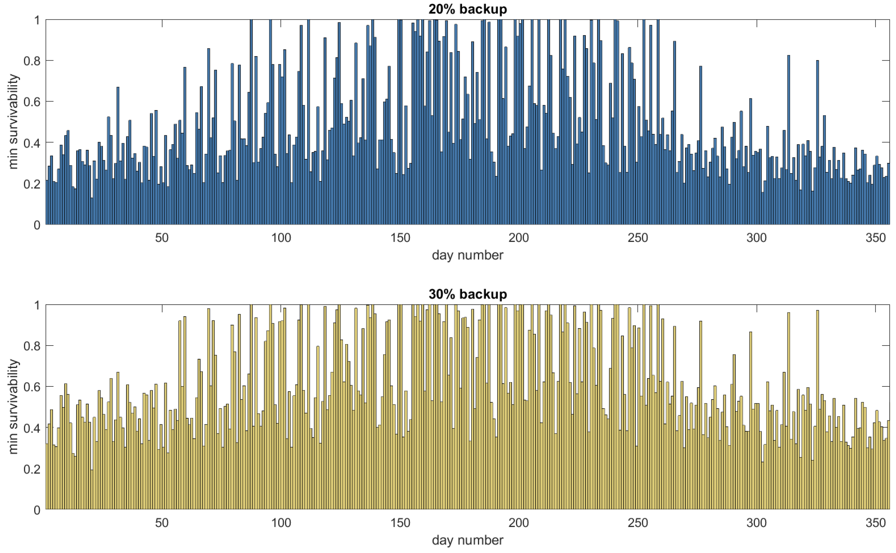
Figure 4 shows the minimum survivability per day for a full year for the smart battery management strategy. The upper figure shows the results when 20% of the battery capacity is reserved as backup, and the lower figure shows similar results for 30% backup capacity. The minimum survivability indicates the probability that the house will survive a grid failure when the failure occurs on the worst possible moment of the day. The worst moment is when the demand is high and the local production and the energy in the battery are low. In Figure 4, we see that the minimum survivability on a day highly depends on the ratio between the production and demand of that day. During the winter, the daily demand is higher than the production. The battery will be at the level of the reserved backup, that is close to 20% or 30% state of charge, at the worst case time of grid failure. This results in a low minimum survivability level. Increasing the backup capacity from 20% to 30% increases the minimum survivability during the winter period by approximately 50%.

In the summer period, during the days with a high production, the battery will be charged during the day. Thus, the survivability level will be much higher. Furthermore, in summer, an increase of the backup capacity results in an increase of the minimum survivability level by approximately 30%. The lower increase in survivability in summer is due to the fact that already, 50% of the days had a survivability that was larger than 70%. Hence, there is less room for improvement. Still, when only 20% of the battery is reserved for backup, the minimum survivability remains below 0.5 for 235 days of the year. When the backup is increased to 30%, this number decreases to 150.

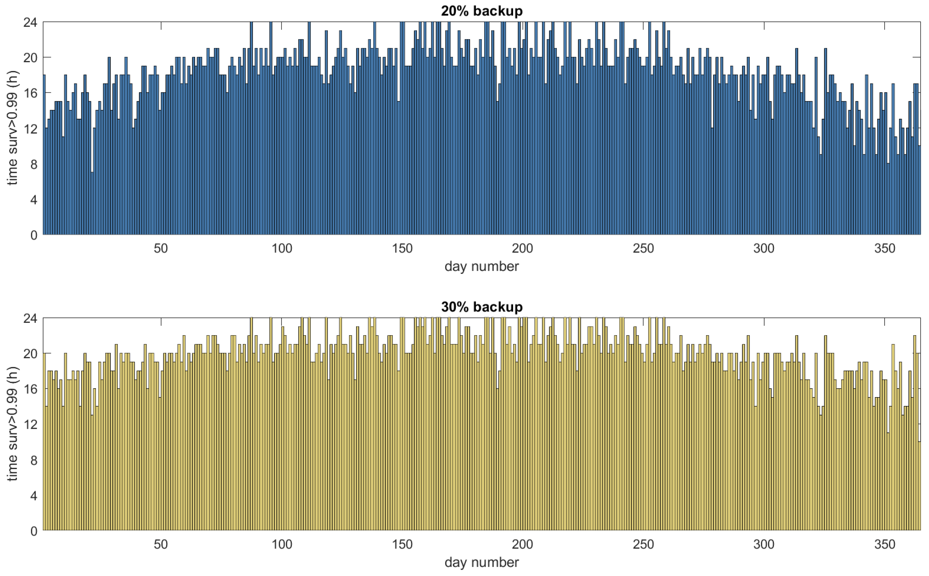
Next to the minimum survivability level, we consider the fraction of time the survivability is above 0.99. Figure 5 shows the number of hours per day that the house is survivable with at least probability 0.99, both for 20% and 30% backup capacity. This measure gives an indication of how likely the house will survive a grid failure at a random point in time with a probability of at least 0.99. In contrast, the minimum survivability is a worst-case measure that may be determined by a very short interval with low available backup capacity.

Figure 5 shows the same trends as Figure 4; during the winter, on average, 13 h of the day have a survivability that is larger than 0.99, when only 20% of the battery is reserved for back up. During the summer, the survivability will be larger than 0.99 on average for 20 h. When the backup capacity is increased to 30%, the time the survivability is larger than 0.99 is increased, especially during winter. Now, for almost all days, the survivability is larger than 0.99 for more than 16 h. For the full year, the fraction of time during which the survivability is larger than 0.99 increases from 0.77 (20% backup) to 0.83 (30% backup).

6.2. Reducing the Demand upon a Grid Failure: The Power-Save Strategy

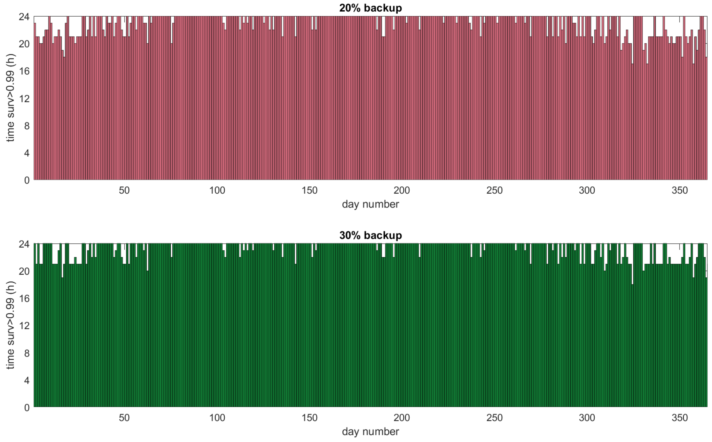
Furthermore, for the power-save strategy, we analyze the minimum survivability per day and the time per day the survivability is larger than 0.99. The results are shown in Figure 6 and Figure 7, respectively.

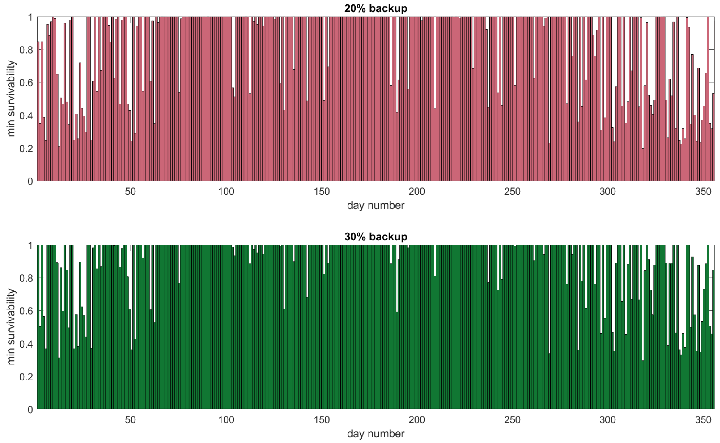
In the power-save strategy, part of the demand is shut down as soon as the grid fails. This clearly improves the survivability of the system. As can be seen in Figure 6, with a backup capacity of 30%, the minimum survivability is close to one for most days in summer. In winter, approximately half of the days have a high minimum survivability, i.e., larger than 0.8. Even though the other days have a minimum survivability of around 0.5 (with a minimum of 0.31), the fraction of time the survivability is above 0.99 is highly increased; see Figure 7. When the backup capacity is increased from 20% to 30%, the fraction of time during one year with a survivability larger than 0.99, is increased from 0.95 to 0.97. This is considerably larger than the results obtained for the smart strategy.

When increasing the reserved backup capacity form 20% to 30%, the smart strategy already increases the minimum hours per day that are survivable from seven to 11; however, using that strategy, we are still left with several days that have a minimum survivability of only $0.19$, even when 30% of the battery is used as backup. The new power-save strategy improves this situation substantially, as it reduces the demand during a grid outage using a prioritization mechanism. Although the new strategy improves the minimum survivability on average significantly, for the worst day of the year, it is still as low as $0.23$ for a 20% backup reservation and $0.29$ for a 30% backup reservation, whereas the minimum number of hours per day that are survivable increases from 17 to 18, respectively.

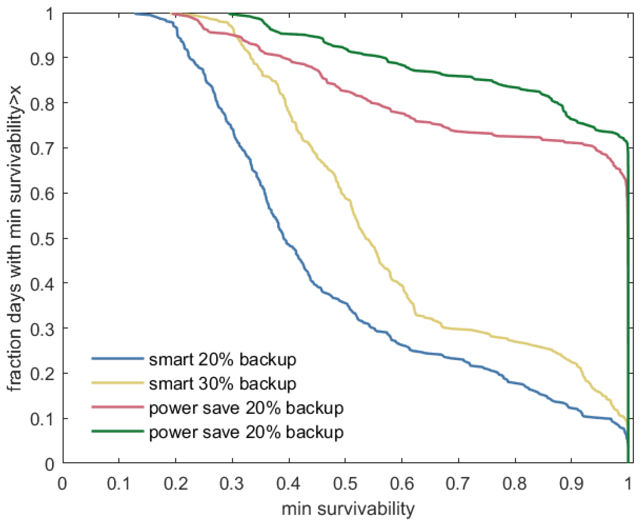
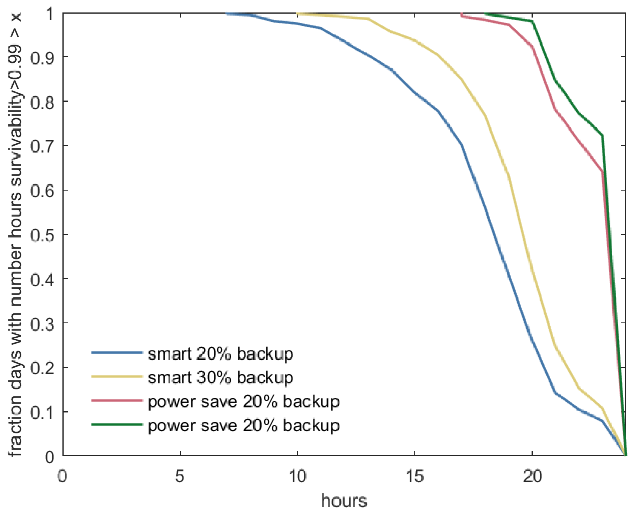
Figure 4, Figure 5, Figure 6 and Figure 7 illustrate the variation of the survivability of the system throughout the year. Even during summer, days with a high minimum survivability may be directly followed by days with a low minimum survivability. However, the figures do not allow for easy comparison between the different strategies. It is especially hard to see the improvements due to a higher level of backup capacity. Therefore, we also plot and analyze the experimental distributions of the minimum survivability per day and the number of hours per day the survivability is larger than 0.99.

Figure 8 shows the fractions of days with a minimum survivability larger than a given threshold, plotted on the x-axis, for the four analyzed strategies. Figure 9 shows the fraction of days for which the survivability is larger than 0.99 for more than a given number of hours. For both plots, we can conclude that a strategy is better when the curve shifts to the top of the figure. In both plots, we can clearly see the improvements obtained by increasing the backup capacity. The improvements are larger for the smart strategy than for the power-save strategy, since the power-save strategy already has a high performance for the 20% backup capacity level. This illustrates the benefit of the power-save strategy, as it is able to deliver a high level of survivability even for a relatively small backup capacity level; it leaves more battery capacity for flexible use.

6.3. Ensuring Survivability All Year Long

Finally, we analyze how much capacity is needed to obtain a given level of survivability throughout the full year. Instead of varying the backup capacity, we now vary the battery capacity itself and set the backup level to 100%, which results in all stored energy being saved for the case of a power outage. This allows us to compute the absolute amount of battery capacity that is needed as backup; in case the full battery capacity should not be used as backup, the actually required size of the battery can be scaled accordingly.

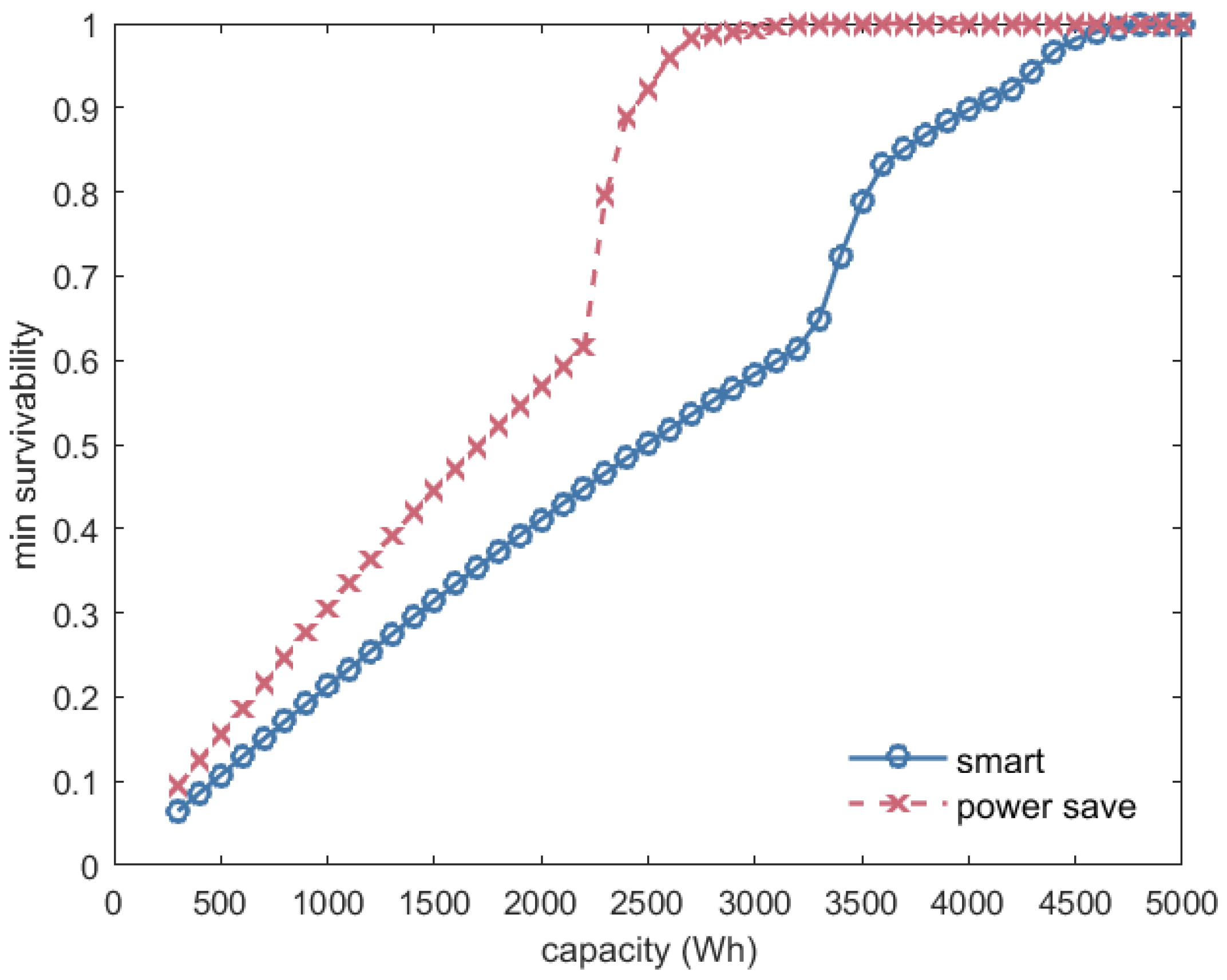
We compute the minimum survivability per year as a function of the battery capacity for both the smart and power-save strategy and for all possible outage occurrences. The results of this analysis are shown in Figure 10.

For a battery with 300 Wh of capacity (the leftmost points in the curves), the minimum survivability is very low for both strategies. The backup capacity is very small; hence, the battery will be empty very fast, and the house will only survive short grid outages. When the battery capacity is increased, the minimum survivability slowly rises for both strategies. The survivability is higher for the power-save strategy, since the reduction of the demand will ensure that the battery can supply the demand longer.

For a battery capacity between 2100 Wh and 2400 Wh, we see a sudden large increase in the survivability level for the power-save strategy. This can be explained as follows. The minimum survivability in the year is determined by the largest peak in the demand. When the battery has enough capacity to supply this peak demand, the survivability level may increase more rapidly, since the remaining battery capacity can supply the lower demand for a longer period of time. A similar effect is seen in the results for the smart strategy around 3500 Wh, although slightly less profound. This is due to the fact that the off-peak demand remains higher in this strategy.

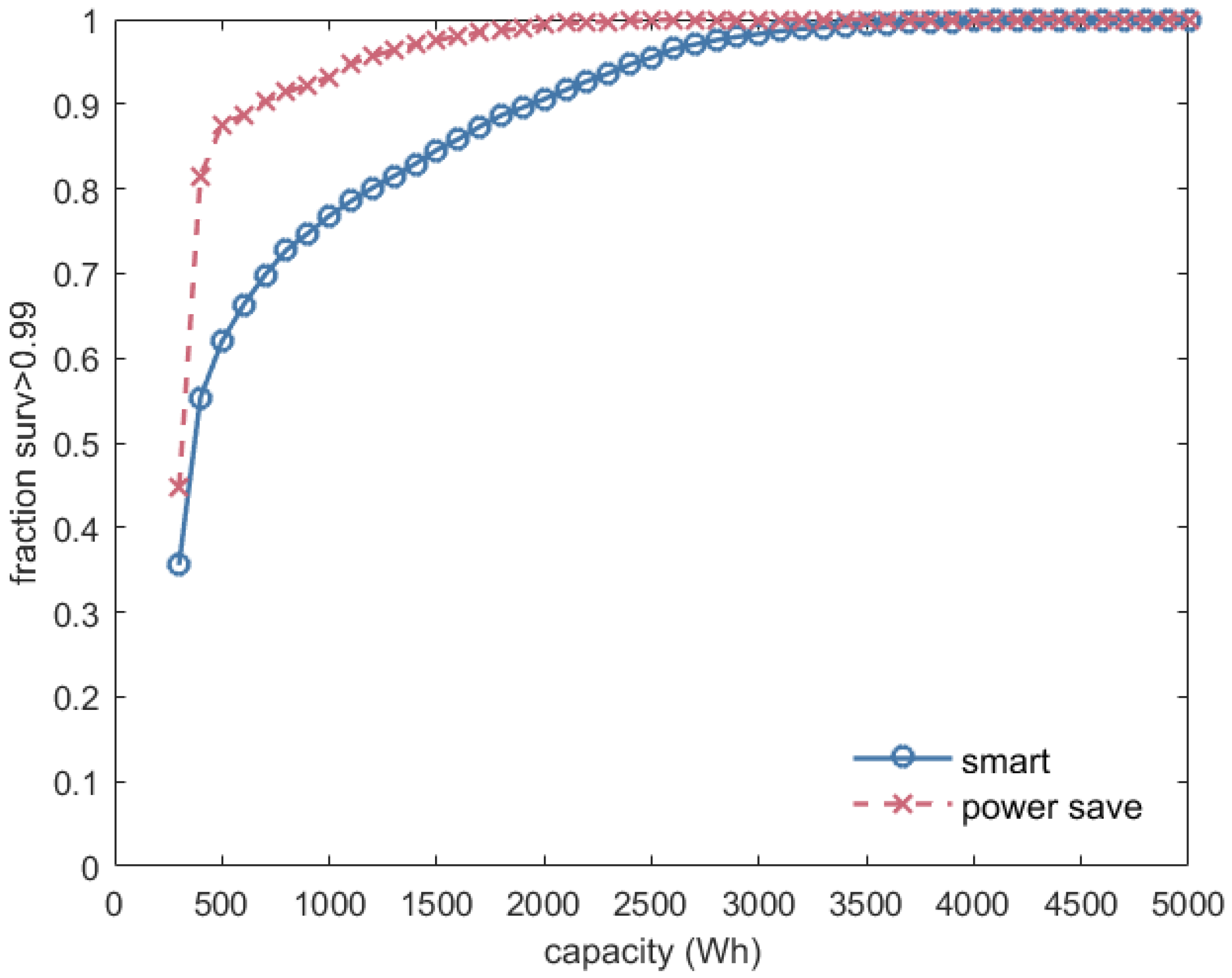
Finally, Figure 11 shows the fraction of the year during which the survivability is larger than 0.99 as a function of the battery capacity. As in Figure 10, the battery is 100% reserved for backup. As can be observed, for a battery of 300 Wh, the system is survivable with a probability of 0.99 for less than 50% of the time; 35% for the smart strategy and 45% for the power-save strategy. When the battery capacity is increased, the fraction of the year the survivability is larger than 0.99 increases rapidly for the power-save strategy. The system has a survivability of larger than 0.99 for 90% of the time with a battery capacity of 700 Wh and for 99% of the time with a battery capacity of 2000 Wh. Note that in order to achieve a system that is always survivable with a probability larger than 0.99, one would need a capacity of 3000 Wh, as shown in Figure 10. Hence, this last 1% is extremely expensive in terms of battery capacity. For the smart strategy, the fraction of the year the system has a survivability larger than 0.99 increases more slowly. For a battery capacity of 2000 Wh, the fraction of time with at least 0.99 survivability is just below 90%. To reach 99%, a battery capacity of 3300 Wh is needed.

When analyzing the minimum survivability as a function of the battery capacity for both strategies, we see that power-save performs much better for battery capacities between 2500 and 3500 Wh. This is quite interesting, since this is a capacity range where batteries are becoming quite affordable; a reasonably-priced battery of 2.7 kWh using power-save results in a very high minimum survivability of 0.99, while the smart strategy still lies at around 0.78 in that case.

7. Conclusions

This paper presents a study of the survivability of a domestic smart energy system in which part of the local battery capacity is reserved for backup purposes in case of grid outages. We analyze this system over a full year, based on simulated electricity generation and demand profiles, made using the ALPG simulator. We analyze, among others, the minimum survivability for each day and the number of hours per day the house is survivable, for two different battery management strategies, smart, which reserves a pre-defined percentage of the battery capacity for backup during grid outages, as well as power-save, which additionally turns off low-priority demand in case of a grid outage.

In contrast to earlier work [15,16], we see that the variability in production and demand per day even within the same season is very large and results in highly different minimum survivability per day. Hence, it is very difficult to guarantee a certain minimum survivability all year round. The newly-introduced power-save strategy leads to a higher survivability on average compared to the smart strategy. Furthermore, with respect to the minimum survivability, power-save outperforms smart, especially for reasonably-sized batteries with a capacity between 2500 and 3500 Wh.

Overall, we show that the variabilities between days even within the same season can have a large impact on the resulting survivability measures and illustrate the added benefit of turning off part of the demand in the case of a grid failure.

In future work, we will investigate adaptive strategies that use weather predictions as part of the battery management system; also, the priority assignment might be adapted based on such forecasts. We will evaluate the impact of such strategies on both the interest of the customer, as well as on the interests of the grid operator. We will also consider to extend our work with more detailed cost considerations, as well as allow for stochastic variations in the demand and generation profiles.

References

- Sterner, M.; Eckert, F.; Thema, M.; Bauer, F. Der positive Beitrag dezentraler Batteriespeicher für eine stabile Stromversorgung; Internal report for Forschungsstelle Energienetze und Energiespeicher (FENES), OTH Regensburg: Regensburg/Berlin/Hannover, Germany, 2015. [Google Scholar]
- Williams, C.; Binder, J.; Danzer, M.; Sehnke, F.; Felder, M. Battery Charge Control Schemes for Increased Grid Compatitbility of Decentralized PV Systems. In Proceedings of the 28th European Photovoltaic Solar Energy Conference, Paris, France, 30 September–4 October 2013; pp. 145–154.
- Ganchinho, M.; Kari, L.; Raut, C. How can utilities survive energy demand disruption? In Accenture’s Digitally Enabled Grid Program; Accenture: Dublin, Ireland, 2014. [Google Scholar]
- McGranaghan, M.; Olearczyk, M.; Gellings, C. Enhancing Distribution Resiliency: Opportunities for Applying Innovative Technologies; Technical Report; Electric Power Research Institute: Palo Alto, CA, USA, 2013. [Google Scholar]
- Van der Klauw, T.; Gerards, M.E.; Smit, G.J.; Hurink, J.L. Optimal scheduling of electrical vehicle charging under two types of steering signals. In Proceedings of the 2014 IEEE PES Innovative Smart Grid Technologies Conference Europe, Istanbul, Turkey, 12–15 October 2014; IEEE Computer Society: Washington, DC, USA; pp. 1–6.
- Bakker, V.; Molderink, A.; Hurink, J.; Smit, G.; Nykamp, S.; Reinelt, J. Controlling and optimizing of energy streams in local buildings in a field test. In Proceedings of the 22nd International Conference and Exhibition on Electricity Distribution (CIRED 2013), Stockholm, Sweden, 10–13 June 2013; pp. 1–4.
- Wang, W.; Xu, Y.; Khanna, M. A survey on the communication architectures in smart grid. Comput. Netw. 2011, 55, 3604–3629. [Google Scholar] [CrossRef]
- Wang, L.; Peng, D.; Zhang, T. Design of Smart Home System Based on WiFi Smart Plug. Int. J. Smart Home 2015, 8, 173–182. [Google Scholar] [CrossRef]
- e-balance consortium. Available online: http://www.e-balance-project.eu (accessed on 5 September 2015).
- Hoogsteen, G.; Molderink, A.; Hurink, J.L.; Smit, G.J. Generation of Flexible Domestic Load Profiles to Evaluate Demand Side Management Approaches. In Proceedings of the IEEE International Energy Conference (Energycon 2016), Leuven, Belgium, 4–8 April 2016; pp. 1–6.
- Ellison, B.; Fisher, D.; Linger, R.; Lipson, H.; Longstaff, T.; Mead, N. Survivable Network Systems: An Emerging Discipline; Technical Report; Carnegie-Mellon Software Engineering Institute: Pittsburgh, PA, USA, 1997. [Google Scholar]
- Cloth, L.; Haverkort, B.R. Model Checking for Survivability. In Proceedings of the Second International Conference on the Quantitative Evaluaiton of Systems, Torino, Italy, 19–22 September 2005; IEEE Computer Society: Washington, DC, USA, 2005; pp. 145–154. [Google Scholar]
- Avritzer, A.; Carnevali, L.; Ghasemieh, H.; Happe, L.; Haverkort, B.R.; Koziolek, A.; Menasche, D.; Remke, A.; Sarvestani, S.S.; Vicario, E. Survivability Evaluation of Gas, Water and Electricity Infrastructure. In Proceedings of the 7th International Workshop on Practical Applications of Stochastic Modelling (PASM 2014), Newcastle, UK, 13 May 2014; Elsevier: Amsterdam, The Netherlands, 2014; pp. 1–20. [Google Scholar]
- Ghasemieh, H.; Remke, A.; Haverkort, B.R. Survivability evaluation of fluid critical infrastructures using Hybrid Petri nets. In Proceedings of the IEEE 19th Pacific Rim International Symposium on Dependable Computing (PRDC 2013), Vancouver, BC, Canada, 2–4 December 2013; pp. 152–161.
- Ghasemieh, H.; Haverkort, B.R.; Jongerden, M.R.; Remke, A. Energy Resilience Modelling for Smart Houses. In Proceedings of the 45th Annual IEEE/IFIP International Conference on Dependable Systems and Networks (DSN 2015), Rio de Janeiro, Brazil, 22–25 June 2015; pp. 275–286.
- Jongerden, M.R.; Hüls, J.; Haverkort, B.R.; Remke, A. Assessing the Cost of Energy Independence. In Proceedings of the IEEE International Energy Conference (Energycon 2016), Leuven, Belgium, 4–8 April 2016; pp. 1–6.
- EDSN. Available online: http://www.edsn.nl/verbruiksprofielen/ (accessed on 3 November 2015).
- NREL. Available online: http://pvwatts.nrel.gov/index.php (accessed on 5 September 2016).
- Hermanns, H.; Wiechmann, H. Future design challenges for electric energy supply. In Proceedings of the IEEE Conference on Emerging Technologies Factory Automation (ETFA 2009), Palma de Mallorca, Spain, 22–25 September 2009; pp. 1–8.
- Hartmanns, A.; Hermanns, H. Modelling and Decentralised Runtime Control of Self-stabilising Power Micro Grids. In Proccesdings of the 5th International Symposium Leveraging Applications of Formal Methods, Verification and Validation. Technologies for Mastering Change (ISoLA 2012), Heraklion, Greece, 15–18 October 2012; Springer: Berlin/Heidelberg, Germany, 2012; pp. 420–439. [Google Scholar]
- Bakker, V.; Bosman, M.G.; Molderink, A.; Hurink, J.L.; Smit, G.J. Improved Heat Demand Prediction of Individual Households. In Proceedings of the first Conference on Control Methodologies and Technology for Energy Efficiency, Vilamoura, Portugal, 29–31 March 2010; Elsevier: Amsterdam, The Netherlands, 2010; pp. 110–115. [Google Scholar]
- Welsch, M.; Howells, M.; Bazilian, M.; DeCarolis, J.; Hermann, S.; Rogner, H. Modelling elements of Smart Grids? Enhancing the {OSeMOSYS} (Open Source Energy Modelling System) code. Energy 2012, 46, 337–350. [Google Scholar] [CrossRef]
- Wang, B.; Sechilariu, M.; Locment, F. Power flow Petri Net modelling for building integrated multi-source power system with smart grid interaction. Math. Comput. Simul. 2013, 91, 119–133. [Google Scholar] [CrossRef]
- Weniger, J.; Tjaden, T.; Quaschning, V. Sizing of Residential PV Battery Systems. Energy Procedia 2014, 46, 78–87. [Google Scholar] [CrossRef]
- Weniger, J.; Bergner, J.; Tjaden, T.; Quaschning, V. Economics of Residential PV Battery Systems in the Self-Consumption Age. In Proceedings of the 29th European Photovoltaic Solar Energy Conference and Exhibition, Amsterdam, The Netherlands, 22–26 September 2014; pp. 1–7.
- Avritzer, A.; Carnevali, L.; Happe, L.; Koziolek, A.; Menasché, D.S.; Paolieri, M.; Suresh, S. A Scalable Approach to the Assessment of Storm Impact in Distributed Automation Power Grids. In Proceedings of the 11th International Conference on Quantitative Evaluation of Systems, (QEST 2014), Florence, Italy, 8–10 September 2014; Springer: Medford, MA, USA, 2014; pp. 345–367. [Google Scholar]
- Chiaradonna, S.; Giandomenico, F.D.; Murru, N. On a Modeling Approach to Analyze Resilience of a Smart Grid Infrastructure. In Proceedings of the Tenth European Dependable Computing Conference (EDCC 2014), Newcastle, UK, 13–16 May 2014; pp. 166–177.
- Rowe, M.; Yunusov, T.; Haben, S.; Holderbaum, W.; Potter, B. The real-time optimisation of DNO owned storage devices on the LV network for peak reduction. Energies 2014, 7, 3537–3560. [Google Scholar] [CrossRef]
- Ferreira, H.; Garde, R.; Fulli, G.; Kling, W.; Lopes, J. Characterisation of electrical energy storage technologies. Energy 2013, 53, 288–298. [Google Scholar] [CrossRef]
- Nguyen, T.; Yoo, H.; Kim, H. Application of Model Predictive Control to BESS for Microgrid Control. Energies 2015, 8, 8798–8813. [Google Scholar] [CrossRef]
- Rahimi, A.; Zarghami, M.; Vaziri, M.; Vadhva, S. A simple and effective approach for peak load shaving using Battery Storage Systems. In Proceedings of the North American Power Symposium (NAPS), Manhatan, KS, USA, 22–24 September 2013.
- Allerding, F.; Mauser, I.; Schmeck, H. Customizable Energy Management in Smart Buildings Using Evolutionary Algorithms. In Applications of Evolutionary Computation; Springer: Berlin/Heidelberg, Germany, 2014; Volume 8602, pp. 153–164. [Google Scholar]
- Van der Klauw, T.; Hurink, J.L.; Smit, G.J.M. Scheduling of Electricity Storage for Peak Shaving with Minimal Device Wear. Energies 2016, 9, 465. [Google Scholar] [CrossRef]
- Tagawa, Y.; Koike, M.; Ishizaki, T.; Ramdani, N.; Oozeki, T.; da Silva Fonseca, J.G.; Masuta, T.; Imura, J.i. Day-ahead scheduling for supply-demand-storage balancing—Model predictive generation with interval prediction of photovoltaics. In Proceedings of the 2015 European Control Conference (ECC), Linz, Austria, 15–17 July 2015; pp. 247–252.
- Sun, C.; Sun, F.; Moura, S.J. Data enabled predictive energy management of a PV-battery smart home nanogrid. In Proceedings of the American Control Conference (ACC), Chicago, IL, USA, 1–3 July 2015; pp. 1023–1028.
- Awad, A.; Bazan, P.; German, R. SGsim: Co-simulation Framework for ICT-Enabled Power Distribution Grids. In Measurement, Modelling and Evaluation of Dependable Computer and Communication Systems; Lecture Notes in Computer Science; Springer: Medford, MA, USA, 2016; Volume 9629, pp. 5–8. [Google Scholar]
- Steber, D.; Bazan, P.; German, R. SWARM: Increasing Households’ Internal PV Consumption and Offering Primary Control Power with Distributed Batteries. In Energy Informatics—4th D-A-CH Conference; Lecture Notes in Computer Science; Springer: Medford, MA, USA, 2015; Volume 9424, pp. 3–11. [Google Scholar]
- KNMI. Available online: http://www.knmi.nl/klimatologie/uurgegevens/ (accessed on 5 September 2016).
- Nedap. Available online: http://www.powerrouter.com/en/ (accessed on 5 September 2016).
- Jongerden, M.R.; Haverkort, B.R. Which battery model to use? IET Softw. 2009, 3, 445–457. [Google Scholar] [CrossRef]
- Postema, B.F.; Remke, A.; Haverkort, B.R.; Ghasemieh, H. Fluid Survival Tool: A Model Checker for Hybrid Petri Nets. In Proceedings of the 17th International GI/ITG Conference, MMB & DFT 2014, Bamberg, Germany, 17–19 March 2014; Springer: Medford, MA, USA, 2014; pp. 255–259. [Google Scholar]
- Council of European Energy Regulators (CEER), Benchmarking Report 5.2 on the Continuity of Electricity Supply, Ref. C14-EQS-62-03. Available online: http://www.ceer.eu/ (accessed on 5 September 2016).
- Union of the Electricity Industry (EURELECTRIC), Power Distribution in Europe Facts & Figures. Available online: http://www.eurelectric.org/media/113155/dsoreport-webfinal-2013-030-0764-01-e.pdf (accessed on 5 September 2016).
© 2016 by the authors; licensee MDPI, Basel, Switzerland. This article is an open access article distributed under the terms and conditions of the Creative Commons Attribution (CC-BY) license (http://creativecommons.org/licenses/by/4.0/).