Evaluation of Rail Potential Based on Power Distribution in DC Traction Power Systems

Abstract

Running rails used as a return conductor and ungrounded scheme have been widely adopted in DC traction power systems. Due to the longitudinal resistance of running rails and insulation resistance of rail-to-ground, there will be a potential rise between running rails and the ground when return current flows through the running rails, which is known as rail potential. At present, abnormal rise of rail potential exists widely in DC traction power systems. The present rail potential model still cannot simulate and explain the abnormal rail potential in the system. Based on the analysis of power distribution with multiple trains running in multiple sections, a dynamic simulation model of rail potential in the whole line is proposed. The dynamic distribution of rail potential and stray current in DC traction power systems when multiple trains run in multiple sections is analyzed, and the impact of traction current distribution on rail potential is evaluated. Simulation results show that the abnormal rise of rail potential during the dynamic operation of the system can be evaluated effectively.

1. Introduction

Direct current (DC) traction power systems with an ungrounded scheme are widely used in urban rail transit lines; the running rails are usually used as return conductor. Due to the longitudinal resistance of running rails, there will be a potential between running rails and the ground when traction current flows back to the traction substation, which is called rail potential. Since the running rails cannot be completely insulated to the ground, some of the return current will leak from running rails into the ground and buried metallic structures, which is known as stray current [1]. At present, abnormal rise of rail potential and stray current exists in many urban railway lines, which may exceed the limit value stipulated in relative standards [2,3]. This will cause damage to human safety and electrochemical corrosion of reinforcing bars and buried metal pipelines [4,5]. In order to guarantee human safety and normal operation of equipment, the regulations to control the rail potential in DC traction power systems should be designed [6,7]. Maximum permissible body voltages as a function of time duration in DC traction systems are provided in IEC 62128-1 [3]. For long-term conditions, the accessible rail potential shall not exceed 120 V. Voltage-limiting devices are usually used to reduce the rail potential by connecting the running rails to the substation ground, in which case the current leakage from voltage-limiting devices can reach 800 A, and the stray current increases significantly. Currently, abnormal rise of rail potential cannot be simulated and evaluated by existing models when multiple trains run in multiple sections. Many anomalies in the line cannot be clarified. For example, rail potential in the first and last sections is much higher than that in the middle sections during the operation of the line. In many lines, rail potential in the first and last sections frequently surpasses the stipulated limits [8]. Although the longitudinal resistance of running rails meets the design requirements, rail potential is still high and inconsistent with the theoretical calculation results. Therefore, the dynamic distribution of rail potential needs further studying when multiple trains run in multiple sections.

There are some studies on controlling the rail potential in DC traction power systems. Relevant studies show that [9,10] reducing the resistance of running rails, improving the voltage level of power supply systems and shortening the distance between traction substations can drop the rail potential effectively. In addition, different grounding schemes of the system—such as solid grounding, diode grounding and being ungrounded—have an impact on rail potential distribution [10]. A number of simulations and experimental results [9] show that the connecting cables between different railway lines are the main cause of high rail potential. What is more, running modes of trains [11], cross-track regeneration supply [12] and other factors also influence the distribution of rail potential and stray current. However, the impact of power distribution on rail potential when multiple trains run in multiple sections has broadly been ignored, and the abnormal rise of rail potential in the actual line has not yet been clarified.

In the last few decades, the simulation model of rail potential and stray current have been studied. The distribution of rail potential is analyzed through finite-element methods and distributed parameter model of return circuit [12,13,14]. Charalambous [12] uses CDEGS software from Safe Engineering Services & Technologies, Ltd. (SES) in Canada to analyze and assess the change of stray current when the cross-track regeneration supply exists. Meanwhile, a topologically accurate model in cut-and-cover sections of DC traction power systems is established to simulate the dynamic distribution of stray current under the influence of train characteristics, time tabling, headway, etc. [13]. In a lumped parameter model of rail potential and stray current [9,14], a segment of 100 m is sufficient and accurate for the simulation, but the conductance matrixes of the whole line will be very large, and speed of the calculation will be slow. In a distributed parameter model of rail potential and stray current [11,15], the impact of power distribution between source nodes and load nodes on rail potential is always ignored. Traction current transmitting over sections exists widely when multiple trains run in multiple sections in DC traction power systems. As stated by Lin [16] and Falvo [17], in DC traction power systems, all traction substations and trains are in parallel operation for the connectivity of the catenary and running rails in the whole line. Traction current of an accelerating train comes not only from the traction substations of the section, but also from traction substations in other sections or regenerative braking trains with a long distance. The current that regenerative braking trains feed back to the catenary can supply power for accelerating trains in other sections. However, little attention has been paid to the power distribution between source nodes and load nodes. Traction current transmitting with a long distance will have an impact on rail potential. The number of nodes in the network of DC traction power systems is large, and the running mode of the traction substation and train can change, becoming very complicated. Subsequently, current flow has many paths. The current distribution between power source nodes and load nodes cannot be drawn exactly by power flow calculation. When multiple trains run in multiple sections, traction current distribution is affected by the parameters of rectifier units, the train’s running modes, as well as the coincidence degree of the trains, parameters of regenerative braking energy absorbing device (RBEAD), line parameters, etc. At present, related l studies [18,19] generally focus on the method of power flow calculation, whereas little attention has been paid to the power flow tracing in a DC traction power system with multiple nodes. Traction current distribution relations between source nodes and load nodes need to be calculated. The impact of traction current distribution on an abnormal rise of rail potential when multiple trains run dynamically in multiple sections is lack of accurate modeling and analysis. For the realization of fast and accurate calculation of rail potential, a new simulation model is proposed in this paper. The simulation model of rail potential consists of the train movement calculation module, power flow calculation module, power flow tracing calculation module and rail potential calculation module.

This paper illustrates the impact of power distribution on rail potential. A dynamic model of rail potential based on power distribution when multiple trains run in multiple sections is established, thereby clarifying the abnormal rise of rail potential in the actual line. Field tests and simulations show that traction current transferring over sections widely exists in DC traction power systems, and the abnormal rise of rail potential during the dynamic operation of the system can be evaluated effectively.

2. System Description

A DC traction power system mainly consists of rectifier units, catenaries, trains, running rails, buried conductor, RBEAD, etc. A schematic of a DC traction power system is shown in Figure 1. For the connectivity of catenaries and running rails in the whole line, all the trains and traction substations are in parallel operation.

The 24-pulse diode rectifier units are usually set in traction substations, which can provide unidirectional current from the alternating current (AC) side to DC side. In this paper, assuming that internal resistance of the rectifier units is changeless, output characteristic of the rectifier units is shown as line I in Figure 2. A train’s running mode can actually be divided into three stages: accelerating, coasting and braking. Regenerative braking is the main braking method, which will feed the current back to the catenary and rise catenary voltage. When the catenary voltage rises to no-load voltage, U₀, of the rectifier units, rectifier units will be out of operation. The output characteristic is shown as line II in Figure 2. If the current that regenerative braking trains feed back to the catenary cannot be fully absorbed by surrounding accelerating trains, then catenary voltage will rise continuously. In order to prevent the catenary voltage from exceeding the safety limit, an RBEAD is usually set in trains or traction substations. When the catenary voltage at RBEAD exceeds its trigger voltage, U_max, the RBEAD will start to absorb the remaining energy so as to ensure that the catenary voltage does not exceed U_max. In the urban railway lines of China, the RBEAD is usually set at traction substations, and its output characteristic is shown as line III in Figure 2. The output characteristic of traction substation with RBEAD is shown in Figure 2.

The train’s traction and regenerative braking curve are constrained by the traction network voltage. With the drop of traction network voltage, train tractive and regenerative braking capacity will be limited [16]. In this paper, the models are simplified without considering the effect of traction network voltage on train traction and braking performance, and it is assumed that the current network voltage can meet the needs of the train traction and braking performance. In the dynamic operation of DC traction power systems, the voltage and current at each node of traction substation or train can be obtained by power flow calculation at each moment. At present, there are many pieces of power flow calculation software for DC traction power systems to obtain the current and voltage at each node [20,21]. Power flow calculation software for DC traction power systems mainly consists of a train movement calculation model and power flow calculation model. With the route parameters, train characteristics, and scheduled timetables, etc., the relation between power and time, as well as the relation between position and time of the trains, can be obtained by the train movement calculation model. Then, parameters such as the current, voltage and power of traction substations and trains at each moment can be attained through the power flow calculation model.

As shown in Figure 1, the return circuit consists of running rails, the buried conductor and the ground. Up line rail and down line rail are connected by cross-bonding cables at intervals of 400 m∼500 m. The buried conductor is set in the ballast bed to collect stray current. The distributed parameters of the return circuit must be converted to lumped parameters for the calculation of power flow. For the realization of fast and accurate calculation of rail potential in this paper, the segment of return circuit between traction substation and train is converted to double π circuit in the power flow calculation. In order to ensure the accuracy of the lumped parameters in double π circuit, the parameters can be calculated by the distributed parameter model [22]. The model in power flow calculation is shown in Figure 3.

As shown in Figure 3, the train is equivalent to a constant power model in the up line or down line, such as P₂ and P₄. P₂ and P₄ are the power of trains at this moment. y_cN is the equivalent resistance of the traction substation. z_r1 and z_s1 are the equivalent resistances of the rail and the buried conductor. y_g1 is the equivalent conductance of rail to buried conductor. y_p1 is the equivalent conductance of buried conductor to the ground. Based on the lumped parameter model at each moment shown in Figure 3, the nodal voltage equations can be obtained, and the power flow can be calculated by iterative methods.

For the realization of fast and accurate calculation of the rail potential, the return circuit between traction substation and train is converted to lumped parameters in the power flow calculation. In order to obtain the rail potential and stray current at each position and evaluate the impact of power distribution on rail potential, the power flow tracing of the system should be calculated, and the rail potential should be calculated by the distributed parameter model of the return circuit.

3. Power Flow Tracing of DC Traction Power Systems

When multiple trains run in multiple sections, the current of each node and branch can be drawn based on power flow calculation at a certain moment. However, it is difficult to obtain the traction current distribution between source nodes and load nodes due to the complexity of the current flow path. The source nodes and load nodes on the catenary at one moment are shown in Figure 4. The current that the regenerative braking train at node 14 feeds back to the catenary can flow to node 7. However, due to the complexity of the path and nodes, it is difficult to calculate the current distribution between nodes 14 and 7. Therefore, it is necessary to trace the power flow in order to obtain the traction current distribution coefficients between the source nodes and the load nodes.

Assuming that there are N nodes on the line at a moment, the traction current distribution coefficient k_ij from the current of source node i, I_Gi, to current of load node j, I_Lj, is shown in Equation (1):

$$I_{ij}=k_{ij}{I}_{Lj}$$

(1)

I_ij is the current from source node i to load node j. The traction current distribution coefficient K of all source nodes and all load nodes is calculated based on the power flow tracing of the DC traction power system.

An analytic model of current distribution in a DC traction power system is established in this paper. In this way, the current distribution relation can be accurately calculated between the power sources and the loads in order to obtain the current and power supply areas.

Assuming that $A={(a_{ij})}_{N\times N}$ is the downstream distribution matrix of a power network with N nodes and I_ij is the current supply from node i to node j by i-j branch, the downstream distribution matrix can be expressed as follows:

$$a_{ij}=\{\begin{array}{cc}-I_{ij}/I_{Tj},& i\ne j,I_{ij}>0\\ 1,& i=j\\ 0,& else\end{array}$$

(2)

where, i, j = 1, 2, 3, …, N. I_Tj is the total injected current of node j.

As shown in Equation (2), the downstream distribution matrix includes the connection relationship between nodes, current flows in branches and the injected current values. The downstream distribution matrix is an unsymmetrical matrix.

$I_L={[I_{L1},I_{L2},\dots ,I_{LN}]}^T$, $I_G={[I_{G1},I_{G2},\dots ,I_{GN}]}^T$ and $I_T={[I_{T1},I_{T2},\dots ,I_{TN}]}^T$ respectively represent the N-dimension load current column vector, source current column vector and total injected current column vector. Based on Kirchhoff’s current law, the input current of each node is equal to the output current, so the vector $I_L$ and $A{I}_T$ can be expressed as:

$$\begin{array}{c}{\displaystyle \sum _{j=1}^N{a}_{ij}{I}_{Tj}=I_{Ti}+{\displaystyle \sum _{j=1,j\ne i,I_{ij}>0}^N\left(\frac{-I_{ij}}{I_{Tj}}\right)}}{I}_{Tj}\\ =I_{Ti}-{\displaystyle \sum _{j=1,j\ne i,I_{ij}>0}^N{I}_{ij}}=I_{Li}\end{array}$$

(3)

where, $i=1,2,\dots ,N$.

It can be expressed as:

$$A{I}_T=I_L$$

(4)

$I_{LL}=diag(I_{L1},I_{L2},\dots ,I_{LN})$, $I_{GG}=diag(I_{G1},I_{G2},\dots ,I_{GN})$ and $I_{TT}=diag(I_{T1},I_{T2},\dots ,I_{TN})$ are the N × N diagonal matrix, $E={[1,1,\dots ,1]}^T$ is the N-dimension unit column vector. The relation of $I_T$ and $I_{TT}$ can be expressed as Equation (5), and the relation of $I_G$ and $I_{GG}$ can be expressed as Equation (6).

$$I_T={[I_{T1},I_{T2},\dots ,I_{TN}]}^T=I_{TT}E$$

(5)

$$I_G={[I_{G1},I_{G2},\dots ,I_{GN}]}^T=I_{GG}E$$

(6)

The analytic relation between $I_G$ and $I_L$ can be expressed as Equation (7).

$$I_G=I_{GG}E=I_{GG}{\left(I_{TT}\right)}^{-1}{I}_T=I_{GG}{\left(I_{TT}\right)}^{-1}{A}^{-1}{I}_L$$

(7)

That is,

$$I_G=I_{GG}{(I_{TT})}^{-1}{A}^{-1}{I}_L$$

(8)

The current distribution between power sources and loads is presented in Equation (8). $I_{GG}{(I_{TT})}^{-1}{A}^{-1}$ is the traction current distribution coefficients. $K=(k_{ij})$, then,

$$K=I_{GG}{(I_{TT})}^{-1}{A}^{-1}$$

(9)

So,

$$I_{Gi}={\displaystyle \sum _{j=1}^N{k}_{ij}{I}_{Lj}}$$

(10)

where, $I_{ij}=k_{ij}{I}_{Lj}$ is the current that the power source at node i supplies for the load at node j.

Based on the current distribution principle, the sum of current distribution coefficients of each power source to all loads should be 1.

The matrix of traction current distribution coefficients meet the relation presented in Equation (11):

$$E^{T}K=E^T{I}_{GG}{I}_{TT}^{-1}{A}^{-1}={\left(I_G\right)}^T{\left(A{I}_{TT}\right)}^{-1}$$

(11)

In order to obtain the property of $K$, the relation between ${\left(I_G\right)}^T$ and $A{I}_{TT}$ should be solved.

Assuming that $B=A{I}_{TT}$, the element at i-th row and j-th column is:

$$B_{ij}=\left(\begin{array}{cccc}{a}_{i1}& a_{i2}& \dots & a_{iN}\end{array}\right)\left[\begin{array}{c}{(I_{TT})}_{1j}\\ {(I_{TT})}_{2j}\\ \dots \\ {(I_{TT})}_{Nj}\end{array}\right]$$

(12)

$I_{TT}$ is a diagonal matrix. Based on $I_{TT}$ and $I_T$, $B_{ij}=a_{ij}{B}_{jj}=a_{ij}{I}_{Tj}$. Based on Equation (2), we can deduce that:

$$B_{ij}=\{\begin{array}{cc}-I_{ij},& i\ne j,I_{ij}>0\\ I_{Tj},& i=j\\ 0,& else\end{array}$$

(13)

Therefore, the sum of elements in j-th column of matrix B is:

$${\displaystyle \sum _{i=1}^N{B}_{ij}=}{\displaystyle \sum _{s=1}^{j-1}{B}_{sj}+B_{jj}+{\displaystyle \sum _{s=j+1}^N{B}_{sj}}}$$

(14)

By the definition of B_ij and I_Tj, we can know that:

$${\displaystyle \sum _{i=1}^N{B}_{ij}=}{\displaystyle \sum _{s=1}^{j-1}{B}_{sj}+I_{Gj}+{\displaystyle \sum _{i,I_{ij}>0}{I}_{ij}}+{\displaystyle \sum _{s=j+1}^N{B}_{sj}}}=I_{Gj}$$

(15)

That is:

$${\left(I_G\right)}^T=E^{T}A{I}_{TT}$$

(16)

Then, $E^{T}K=E^T{I}_{GG}{I}_{TT}^{-1}{A}^{-1}={\left(I_G\right)}^T{\left(A{I}_{TT}\right)}^{-1}=E^T$, and the sum of each column element is 1, which complies with the current distribution principle.

Based on the above method, the current distribution of all power sources and loads at a moment can be obtained in DC traction power systems.

4. Modeling of Rail Potential

In DC traction power systems, multiple trains run in multiple sections. The current at load node comes from many power sources, and each power source supplies power to many load nodes simultaneously. On the basis of traction current distribution coefficients, the line consists of multiple power supply sections. The return circuit is a linear model, and it follows linear superposition theorem. The rail potential with multiple trains running in multiple sections can be obtained by superimposing the rail potential of each power supply section in the line, assuming that the total length of the line is L and there are N nodes in the line. The direction of 0 to L is the positive value of current in running rails. The positive current of the traction substation and train indicates that the current is injected to the rail. The power supply section from j-th source node to i-th load node is shown in Figure 5a. The traction current that I_Gj supplies for I_Li is $I_{ji}=k_{ji}{I}_{Gj}$, the position of j-th source node is x_j and the position of i-th load node is x_i.

Assuming that a single power supply section exists in x_i to x_j, and the supply current is k_jiI_Gj, then the rail potential in the line is divided into three continuous change sections. The distributed parameter model of the return circuit at any point between x to (x + dx) is shown in Figure 5b.

As shown in Figure 5b, u_rij(x), u_sij(x), i_rij(x) and i_sij(x) respectively represent rail potential, potential of buried conductor to the ground, current in rail and stray current in buried conductor at position x. Based on Kirchhoff’s law, these parameters meet the following equation:

$$\{\begin{array}{l}\frac{d{u}_{rij}(x)}{dx}=-R_r\cdot i_{rij}(x)\\ \frac{d{u}_{sij}(x)}{dx}=-R_s\cdot i_{sij}(x)\\ \frac{d{i}_{rij}(x)}{dx}=-G_s\cdot u_{rij}(x)+G_s\cdot u_{sij}(x)\\ \frac{d{i}_{sij}(x)}{dx}=G_s\cdot u_{rij}(x)-(G_p+G_s)\cdot u_{sij}(x)\end{array}$$

(17)

where, R_r is the longitudinal resistance of the running rail, Ω/km; R_s is the longitudinal resistance of the buried conductor, Ω/km; G_s is the longitudinal insulation conductance of rails to the buried conductor, S/km; G_p is the longitudinal insulation conductance of the buried conductor to the ground, S/km.

Due to the different boundary conditions of three sections, the undetermined coefficient of rail potential is different in the three sections.

The parameters in section 0 to x_i can be expressed as follows:

$$\left[\begin{array}{l}{u}_{rij1}(x)\\ u_{sij1}(x)\\ i_{rij1}(x)\\ i_{sij1}(x)\end{array}\right]=H\times \left[\begin{array}{l}{C}_{ij1}{e}^{-\alpha x}\\ C_{ij2}{e}^{\alpha x}\\ C_{ij3}{e}^{-\beta x}\\ C_{ij4}{e}^{\beta x}\end{array}\right],0\le x<x_i$$

(18)

The parameters in section x_i to x_j can be expressed as follows:

$$\left[\begin{array}{l}{u}_{rij2}(x)\\ u_{sij2}(x)\\ i_{rij2}(x)\\ i_{sij2}(x)\end{array}\right]=H\times \left[\begin{array}{l}{C}_{ij5}{e}^{-\alpha x}\\ C_{ij6}{e}^{\alpha x}\\ C_{ij7}{e}^{-\beta x}\\ C_{ij8}{e}^{\beta x}\end{array}\right],x_i\le x<x_j$$

(19)

The parameters in section x_j to L can be expressed as follows:

$$\left[\begin{array}{l}{u}_{rij3}(x)\\ u_{sij3}(x)\\ i_{rij3}(x)\\ i_{sij3}(x)\end{array}\right]=H\times \left[\begin{array}{l}{C}_{ij9}{e}^{-\alpha x}\\ C_{ij10}{e}^{\alpha x}\\ C_{ij11}{e}^{-\beta x}\\ C_{ij12}{e}^{\beta x}\end{array}\right],x_j\le x\le L$$

(20)

where, $H=\left[\begin{array}{cccc}1& 1& 1& 1\\ 1-\frac{{\alpha }^2}{G_s{R}_r}& 1-\frac{{\alpha }^2}{G_s{R}_r}& 1-\frac{{\beta }^2}{G_s{R}_r}& 1-\frac{{\beta }^2}{G_s{R}_r}\\ \frac{\alpha }{R_r}& -\frac{\alpha }{R_r}& \frac{\beta }{R_r}& -\frac{\beta }{R_r}\\ r_{\alpha }& -r_{\alpha }& r_{\beta }& -r_{\beta }\end{array}\right]$, $r_{\alpha }=\frac{G_p}{\alpha }-\frac{\alpha }{R_r}-\frac{G_p\alpha }{G_s{R}_r}$, $r_{\beta }=\frac{G_p}{\beta }-\frac{\beta }{R_r}-\frac{G_p\beta }{G_s{R}_r}$, $\alpha =\sqrt{\frac{m+n}{2}+\sqrt{\frac{{(m-n)}^2}{4}+mk}}$, $\beta =\sqrt{\frac{m+n}{2}-\sqrt{\frac{{(m-n)}^2}{4}+mk}}$, $m=G_s{R}_r$, $n=R_s(G_s+G_p)$, and $k=R_s{G}_s$. C_ij1~C_ij12 are the undetermined coefficients that can be obtained by the boundary conditions in each section.

C_ij1~C_ij12 can be obtained by Equation (21) as follows:

$$\{\begin{array}{l}{i}_{rij1}(0)=0\\ -i_{rij1}(x_i)+i_{rij2}(x_i)=k_{ji}{I}_{Gj}\\ u_{rij1}(x_i)=u_{rij2}(x_i)\\ i_{rij2}(x_j)-i_{rij3}(x_j)=k_{ji}{I}_{Gj}\\ u_{rij2}(x_j)=u_{rij3}(x_j)\\ i_{rij3}(L)=0\\ i_{sij1}(0)=0\\ i_{sij1}(x_i)=i_{sij2}(x_i)\\ u_{sij1}(x_i)=u_{sij2}(x_i)\\ i_{sij2}(x_j)=i_{sij3}(x_j)\\ u_{sij2}(x_j)=u_{sij3}(x_j)\\ i_{sij3}(L)=0\end{array}$$

(21)

Then, the u_rij(x), u_sij(x), i_rij(x) and i_sij(x) can be obtained when a power supply section from x_i to x_j exists in the line.

There may be up to N × N power supply sections in the line, and the return circuit is a linear model, which meets the linear superposition theorem. At a certain time, the rail potential with multiple trains running in multiple sections can be obtained by Equation (22), and other parameters can be attained by Equations (23)–(25).

$$u_r(x)={\displaystyle \sum _{i=1}^N{\displaystyle \sum _{j=1}^N{u}_{rij}(x)}}$$

(22)

$$u_p(x)={\displaystyle \sum _{i=1}^N{\displaystyle \sum _{j=1}^N{u}_{pij}(x)}}$$

(23)

$$i_r(x)={\displaystyle \sum _{i=1}^N{\displaystyle \sum _{j=1}^N{i}_{rij}(x)}}$$

(24)

$$i_s(x)={\displaystyle \sum _{i=1}^N{\displaystyle \sum _{j=1}^N{i}_{sij}(x)}}$$

(25)

Then, the distribution of rail potential and stray current can be simulated with multiple trains running in multiple sections at each moment.

The flow chart of simulation on rail potential dynamic distribution in this paper is shown in Figure 6. It mainly consists of four modules: the train movement calculation module, the power flow calculation module, the power flow tracing module and the rail potential module. Based on the route parameters, train characteristics, and scheduled timetables, the power and position of each train changing with time can be obtained by the train movement calculation module. At each time point, the segment of return circuit between traction substation and train is converted to lumped parameters. The voltage and current of each node in the network can be calculated by the power flow calculation module. For the nonlinear output characteristics of traction substations with RBEAD, the iterative method is usually used in power flow calculations. In each iteration, the operation state of the traction substation may change based on the catenary voltage. Based on the actual characteristic of the line, if more than one traction substation needs to change the operation state, only one traction substation is permitted to change the operation state in this iteration. The iteration will continue until the i-th step when the power-balance equations $\Delta P_n<{\epsilon }_1$ and mismatch voltage of each node $\Delta U_n<{\epsilon }_2$ are all fulfilled. Then, distribution of rail potential at this time point can be drawn by the power flow tracing module and rail potential module. The simulation will continue until the time exceeds the limit t_end. By this model, the dynamic distribution of the rail potential when multiple trains run in multiple sections with different train diagrams and line parameters can be simulated.

5. Simulation Results

Take the first-stage project of Guangzhou Metro Line 2 as an example to simulate the dynamic distribution of rail potential based on the method proposed in this paper. The parameters in the simulation are shown in

Table 1. Simulation Parameters.

Parameter	Value
Equivalent resistance of the traction substation ycN/(Ω)	0.008
No-load voltage of the traction substation U0/(V)	1593
Trigger voltage of regenerative braking energy absorbing device Umax/(V)	1800
Longitudinal resistance of the catenary Rw/(Ω/km)	0.02
Longitudinal resistance of the running rail Rr/(Ω/km)	0.02
Longitudinal resistance of the buried conductor Rs/(Ω/km)	0.02
Longitudinal insulation conductance of rails to buried conductor Gs/(S/km)	1/15
Longitudinal insulation conductance of the buried conductor to the ground Gp/(S/km)	1/3
Mismatch power in the iteration ξ1/(kW)	10−4
Mismatch voltage of each node in the iteration ξ2/(V)	10−4

.

In the first-stage project of Guangzhou Metro Line 2, cross-bonding cables exist between the running rails of up line and down line. The catenaries of up line and down line are connected by positive buses at the position of traction substation, and they are independent in the interval. There are ten stations in the first-stage project of Guangzhou Metro Line 2. The locations of the stations are shown in

Table 2. Locations of the Stations.

Station	Guangzhou Nan(S1)	Shibi	Huijiang (S2)	Nanpu	Luoxi (S3)
Position/m	0	1020	3367	5800	6994
Station	Nanzhou	Dongxiao Nan(S4)	Jiangtailu	Changgang	Jiangnan Xi(S5)
Position/m	9387	10,291	12,265	13,171	14,042

.

Five traction substations, S₁ to S₅, are respectively set in Guangzhou Nan Station, Huijiang Station, Luoxi Station, Dongxiao Nan Station and Jiangnan Xi Station. Other stations are train stations without rectifier units and RBEAD. The train headway is 180 s in the up line and down line, and the dwell time of each train at each station is 30 s. The time step in the simulation is 0.5 s. In the simulation, the parameters of all trains in line are assumed to be the same. According to the operation characteristics of metro systems, the traffic will be regular from the time when the train diagram is stable. In the simulation, the train headway is 180 seconds in the up line and down line, and a train needs 1078 s to run from the departure station to the terminal station. There will be six trains at most in the whole line. Therefore, from the time of seventh train starting from the departure station, each 180 s demonstrate t cyclic behavior. Thus, the simulation can be carried out from 1080 s to 1260 s. In order to compare the current distribution in different situations, the simulation time in this paper is from 0 s to 1260 s.

The position-time curve of each train in the course of simulation is shown in Figure 7.

5.1. Model Validation

For the model validation, field tests of the rail potential were carried out on 16 August 2016, when two trains were tested in the line. In the field tests, two diagrams of the trains were used. In diagram 1, train 1 accelerated from Dongxiao Nan Station in the up line at 26 s, while train 2 accelerated from Nanpu Station in the down line at the same time. In diagram 2, train 1 accelerated from Dongxiao Nan Station in the up line at 0 s, and it began to brake at 38 s; train 2 accelerated from Nanpu Station in the down line at 26 s. The regenerative braking train was in high coincidence with the accelerating train in diagram 2. The simulation results comparing with field test results in two diagrams are shown in Figure 8. The field test point is set at Nanpu Station.

As shown in Figure 8, the simulation results show the same trend with the field test results. The maximum value of the rail potential in field tests is higher than the simulation results. This situation may be caused by the increase of rail longitudinal resistance during the operation. In diagram 1, two trains accelerated at the same time. There is no regenerative braking current in the line, and the traction current of the train was supplied by the traction substations with a short distance. The maximum rail potential at Nanpu Station in the field test was 42.9 V. When the train in regenerative braking was in high coincidence with the accelerating train in diagram 2, the rail potential changed significantly. As shown in Fig. 8b, train 2 accelerated from Nanpu Station in the down line at 26 s. Train 1 in the up line began to brake at 38 s, and fed the regenerative energy back to the catenary. The maximum value of rail potential in the field test was 94.2 V, occurring at 42 s when train 1 was in regenerative braking. In diagram 2, the rail potential rose starkly when the accelerating train and regenerative braking train were in high coincidence. From the comparison of the simulation results and field test results, we can see that the simulation model can evaluate the rail potential effectively in the actual line.

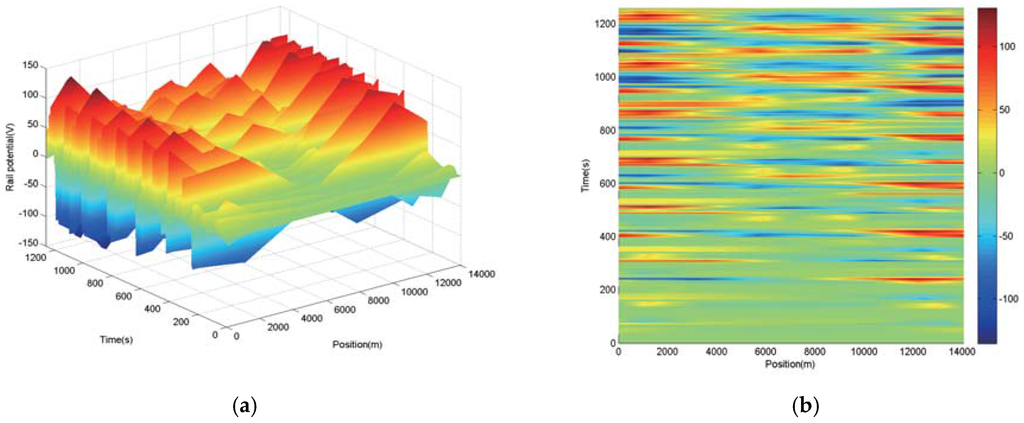
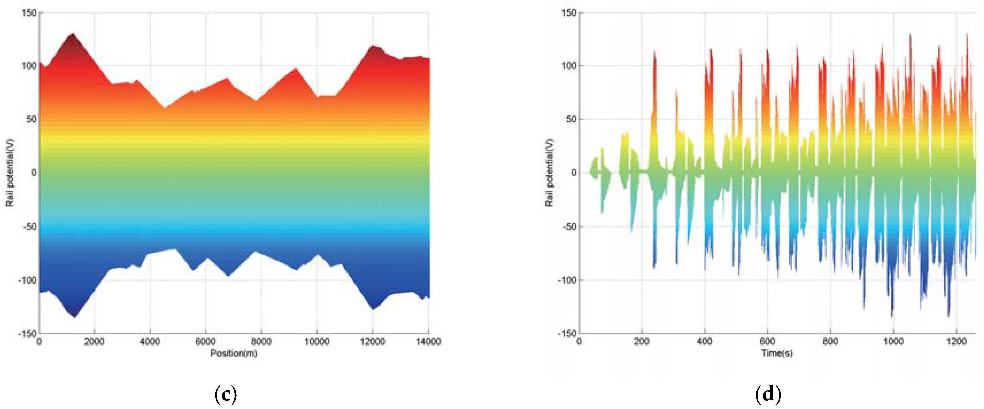
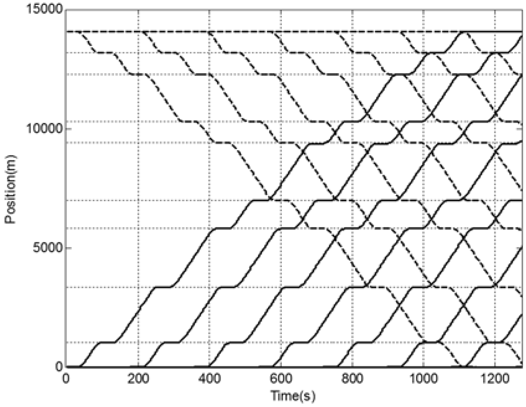
5.2. Effect of Power Distribution on Rail Potential

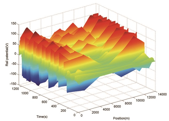
During the simulation time, the dynamic distribution of the rail potential in the line is as shown in Figure 9.

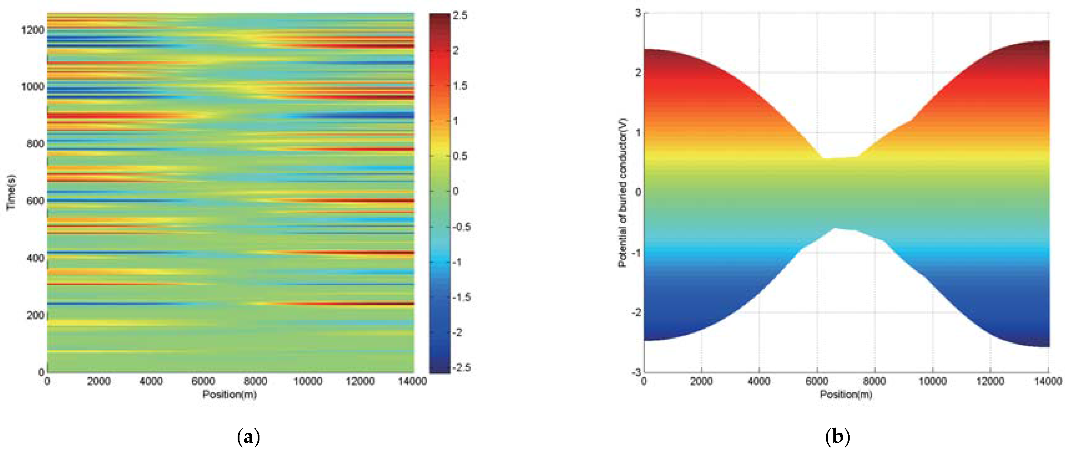
As shown in Figure 9, a significant difference between rail potential exists in different times and positions. The maximum rail potential in the line is 130.8 V, occurring in 1230 m at 1231 s. As shown in Figure 9c, the simulation result of rail potential is consistent with the distribution in the actual line. The rail potential in the first and last sections is much higher than that in the middle sections during the operation of the line. The maximum and minimum values of the rail potential in each section and traction substation are shown in

Table 3. Maximum and Minimum Rail Potential in Each Section and Traction Substation.

Position	S1	Section1 (3367 m)	S2	Section2 (3627 m)	S3	Section3 (3297 m)	S4	Section4 (3751 m)	S5
Maximum (V)	103.3	130.8	83.7	88.6	80.6	98.0	72.3	119.3	107.3
Minimum (V)	−102.8	−135.2	−85.9	−96.7	−92.0	−92.0	−81.8	−127.9	−116.5

.

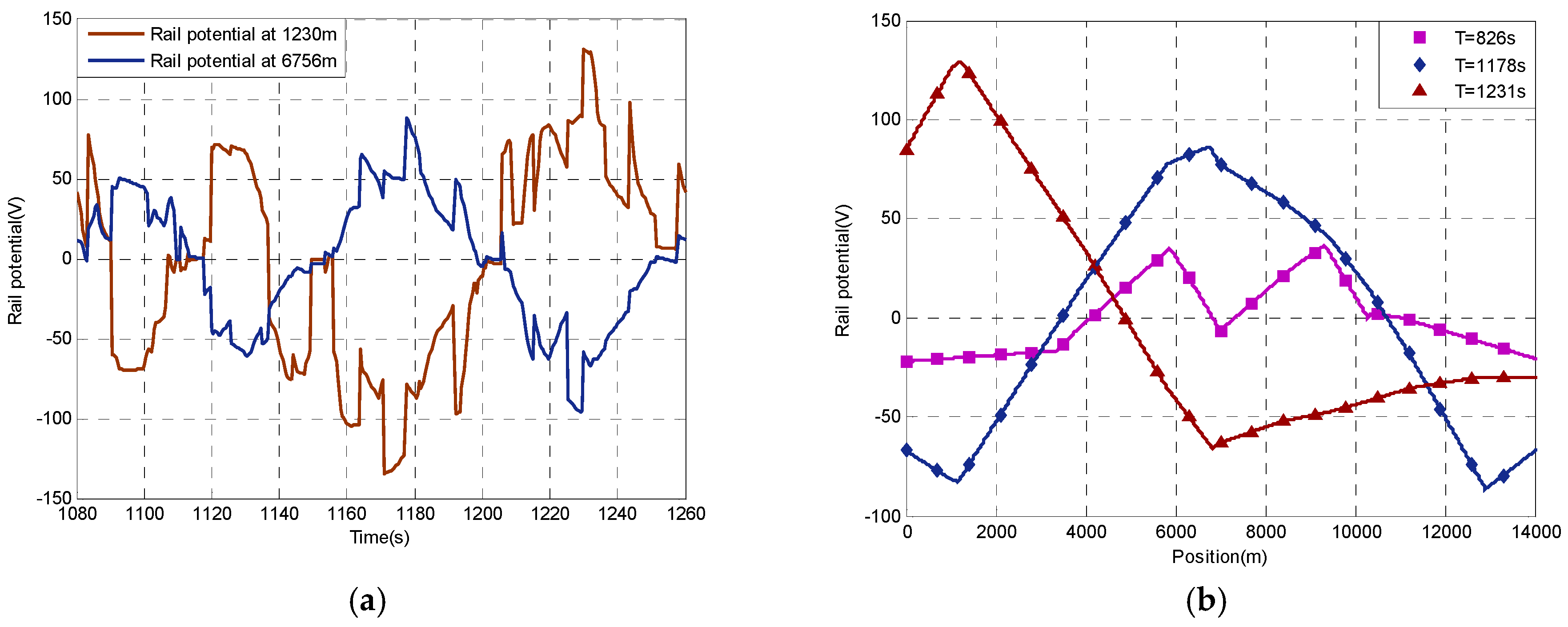
As clearly shown in Table 3, the rail potential in the first and last sections is higher than that in the middle sections. With the same parameters of the return circuit, the length of section 1 is 3367 m, and the maximum rail potential in section 1 is 130.8 V. By comparison, the length of section 2 is 3627 m, whereas the maximum rail potential is 88.6 V. From 1080 s to 1260 s, the maximum rail potential in section 1 is 130.8 V, occurring in 1230 m at 1231 s, and the maximum rail potential in section 2 is 88.6 V, occurring in 6756 m at 1178 s. Variation of the rail potential at typical moments and positions are shown in Figure 10.

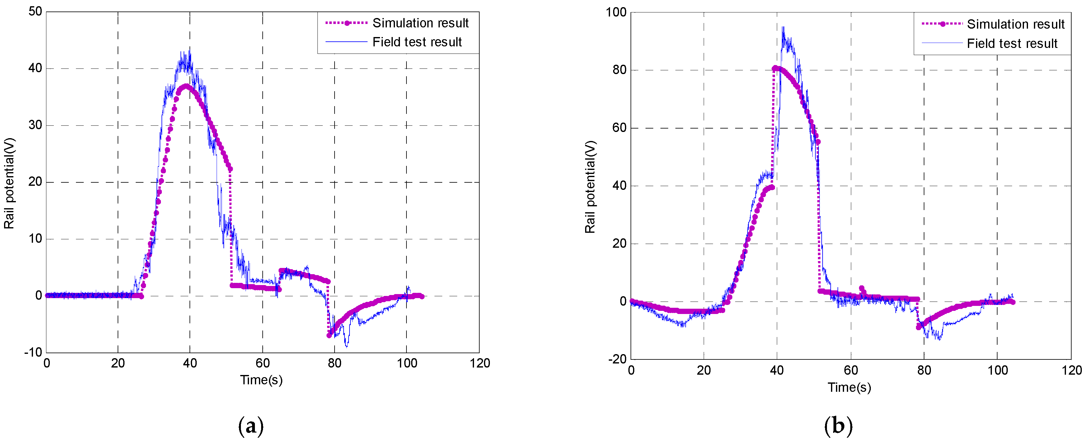
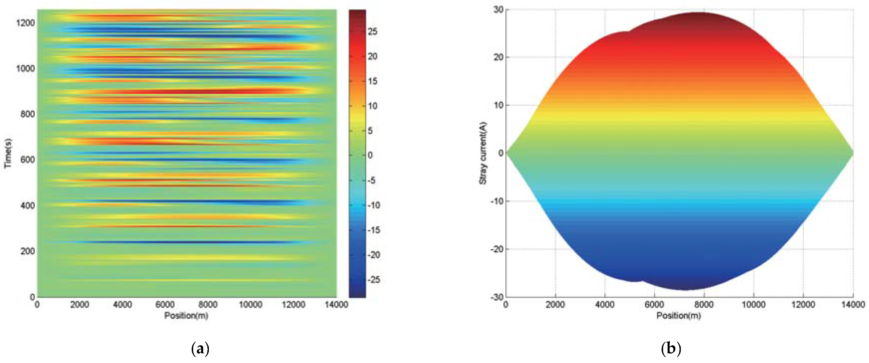
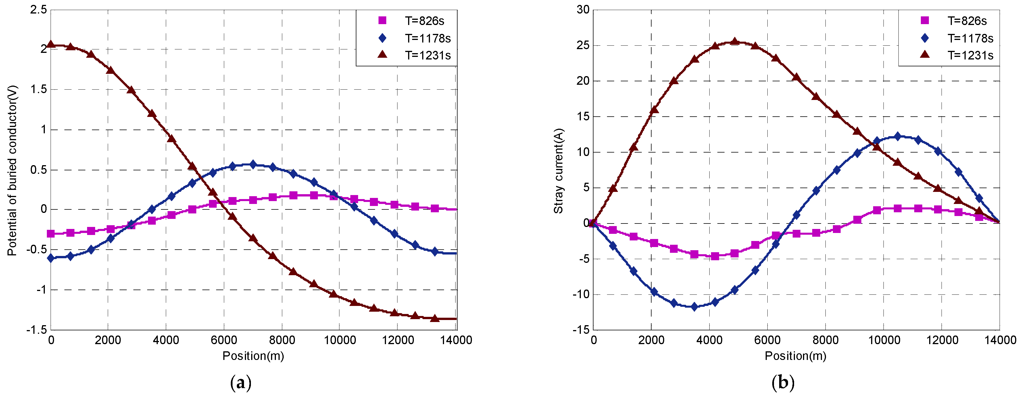
As shown in Figure 10a, at 1230s, the rail potential at the position of 1230 m is 89.3 V. When a train in section 2 begins regenerative braking at 1231 s, the rail potential reaches 130.8 V rapidly with the increase of the traction current transferring over the section. At 1177 s, the rail potential at 6756 m is 49.3 V. When a train in section 4 begins regenerative braking at 1178 s, the rail potential rises to 88.6 V with the increase of the traction current transferring over the section. During the period of the train in regenerative braking, the rail potential remains at a high level, and changes with the traction current transfers over the sections. It can be seen that rail potential is highly affected by the power distribution. As shown in Figure 10b, although the rail potentials at 1231 s and 1178 s are influenced by traction current transferring over sections, the maximum value in section 1 is much higher than that in section 2. Therefore, it is necessary to analyze the power distribution and rail potential at the two typical moments and positions. Meanwhile, the power distribution and rail potential at the time of 826 s is analyzed as a comparison. At 826 s, the total traction current is large, but there are no trains in regenerative braking in the line, and the traction current transferring over sections is low. The maximum rail potential in the line at 826 s is 35.3 V.

Table 4. Positions and Current of the Trains and Traction Substations at 1231 Seconds.

Symbol	S1	Tu1	Td6	Tu2	S2	Td5	Tu3	Td4	S3	Tu4	Td3	S4	Tu5	Td2	Tu6	Td1	S5
Current(A)	−2022.5	1187.2	2581.1	0	0	180.3	−398.6	−2349	444.2	167.4	−95.0	0	−35.4	169.8	170.5	0	0
Position(m)	0	1009	1230	3367	3367	4034	5801	6828	6994	8391	9383	10,291	10,293	11,274	12,821	13,171	14,042

shows the positions and current of all the trains and traction substations at 1231 s in the line.

As shown in Table 4, there are six trains, T_u1~T_u6, in the up line and there are six trains, T_d1~T_d6, in the down line at 1231 s. At this moment, T_u2 and T_d1 stop respectively at Huijiang Station and Changgang Station with a traction current of 0 A. Traction substations S₂, S₄ and S₅ are out of operation. The current distribution between the power sources and the loads are shown in

Table 5. Current Distribution at 1231s.

Source	Load(A)
	Tu1	Td6	Td5	S3	Tu4	Td2	Tu6	Total(A)
S1	607.7	1414.8	0	0	0	0	0	2022.5
Tu3	132.3	266.3	0	0	0	0	0	398.6
Td4	447.2	900.0	180.3	444.2	167.4	116.9	93	2349
Td3	0	0	0	0	0	52.9	42.1	95
Tu5	0	0	0	0	0	0	35.4	35.4
Total(A)	1187.2	2581.1	180.3	444.2	167.4	169.8	170.5

.

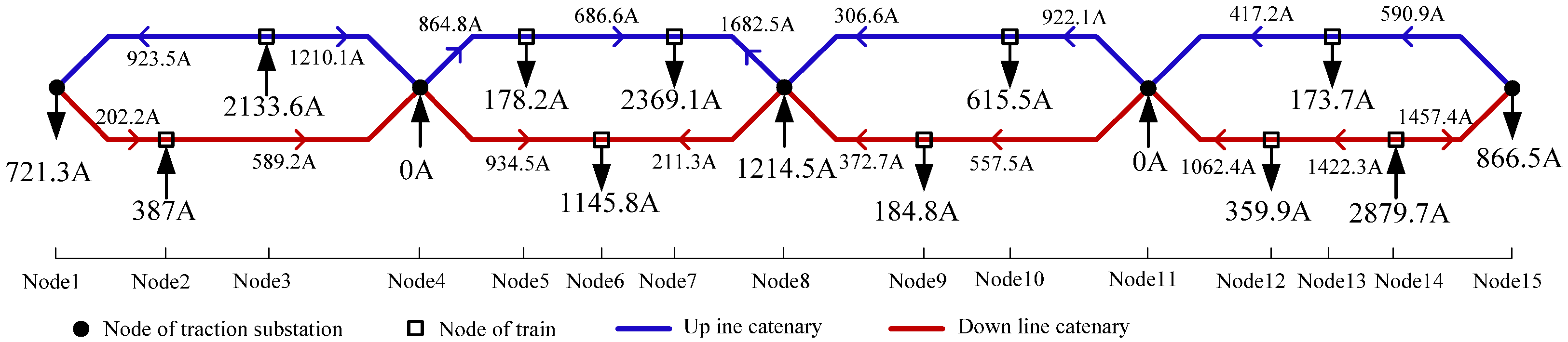
As shown in Table 5, in the traction current of accelerating train T_d6 at 1230 m, 1414.8 A comes from traction substation S₁ with the distance of 1230 m; 266.3 A comes from the regenerative braking train T_u3 with the distance of 4571 m; 900.0 A comes from the regenerative braking train T_d4 with the distance of 5598 m.

Table 6. Positions and Current of the Trains and Traction Substations at 1178 s.

Symbol	S1	Td6	Tu1	Td5	S2	Tu2	Td4	Tu3	S3	Td3	Tu4	S4	Td2	Tu5	Td1	Tu6	S5
Current(A)	721.3	−387	-2133.6	0	0	178.2	1145.8	2369.1	−1214.5	184.8	615.5	0	359.9	173.7	−2879.7	0	866.5
Position(m)	0	1016	1164.0	3367	3367	3949	5808	6756	6994	8475	9390	10,291	10,294	11,189	12,905	13,171	14,042

shows the positions and current of all the trains and traction substations at 1178 s in the line.

Table 6 illustrates the current and positions of all trains and traction substations at 1178 s. At this moment, there are six trains, T_u1~T_u6, in the up line and there are six trains, T_d1~T_d6, in the down line. T_d5 and T_u6 stop respectively at Huijiang Station and Changgang Station; traction substations S₂ and S₄ are out of operation. The RBEAD at substations S₁ and S₅ are activated to absorb the remaining braking energy. The traction current distribution between the power sources and the loads are shown in

Table 7. Current Distribution at 1178s.

Source	Load(A)
	S1	Tu2	Td4	Tu3	Td3	Tu4	Td2	Tu5	S5	Total(A)
Td6	0	38.3	201	147.7	0	0	0	0	0	387
Tu1	721.3	139.9	733.5	538.9	0	0	0	0	0	2133.6
S3	0	0	141.3	1073.2	0	0	0	0	0	1214.5
Td1	0	0	70	609.3	184.8	615.5	359.9	173.7	866.5	2879.7
Total(A)	721.3	178.2	1145.8	2369.1	184.8	615.5	359.9	173.7	866.5

.

As shown in Table 7, in the traction current of accelerating train T_u3 at 6756 m, 147.7 A comes from the regenerative braking train T_d6 with the distance of 5740 m, 538.9A comes from the regenerative braking train T_u1 with the distance of 5592 m, 1073.2 A comes from the traction substation S₃ with the distance of 238 m, 609.3 A comes from the regenerative braking train T_d1 with the distance of 6149 m.

Table 8. Positions and Current of the Trains and Traction Substations at 826 s.

Symbol	S1	Td5	Td4	S2	Tu1	Td3	Tu2	S3	Td2	Tu3	S4	Td1	Tu4	Tu5	S5
Current (A)	−82.2	0	0	−1105.7	189.7	2810.8	192.3	−2985.4	194.7	2696.8	−4207.4	2451.3	191.4	0	−346.3
Position (m)	0	1020	3367	3367	3771	5886	6581	6994	8653	9330	10,291	10,345	11,011	13,168	14,042

shows the positions and current of all the trains and traction substations at 826 s in the line.

Table 8 illustrates the current and positions of all trains and traction substations at 826 s. At this moment, the maximum rail potential in the line is 35.3 V. There are five trains T_u1~T_u5 in the up line and five trains, T_d1~T_d5, exist in the down line. T_d5, T_d4 and T_u5 stop respectively in Shibi Station, Huijiang Station, and Changgang Station. The current distribution between the power sources and the loads are shown in

Table 9. Current Distribution at 826 s.

Source	Load (A)
	Tu1	Td3	Tu2	Td2	Tu3	Td1	Tu4	Total (A)
S1	13.1	64.2	4.9	0	0	0	0	82.2
S2	176.6	863.8	65.3	0	0	0	0	1105.7
S3	0	1882.8	122.1	145.8	834.7	0	0	2985.4
S4	0	0	0	48.9	1862.1	2279	17.4	4207.4
S5	0	0	0	0	0	172.3	174	346.3
Total(A)	189.7	2810.8	192.3	194.7	2696.8	2451.3	191.4

.

As shown in Table 9, the total traction current of all the accelerating trains in line is 8727.2 A, whereas the total traction current is respectively 4456.3 A at 1231 s and 5027 A at 1178 s. However, the maximum rail potential at 826s is much lower than that at 1231 s and 1178 s. Although the total traction current is high at 826 s, there are no regenerative braking trains in the line at this moment. The traction current of accelerating trains comes from the traction substations with a short distance. In the traction current of the accelerating train T_d3 at 5886 m, 1882.8 A comes from the traction substation S₃ with the distance of 1108 m; 863.8 A comes from the traction substation S₂ with the distance of 2519 m; and 64.2 A comes from S₁ with the distance of 5886 m. In the traction current of the accelerating train T_u3 at 5933 m, 834.7 A comes from the traction substation S₃ with the distance of 2336 m; and 1862.1 A comes from the traction substation S₄ with the distance of 961 m. In the traction current of the accelerating train T_d1 at 10,345 m, 2279 A comes from the traction substation S₄ with the distance of 54 m, and 172.3 A comes from the traction substation S₅ with the distance of 3697 m.

Comparing the distribution of traction current and rail potential at 826 s, 1178 s and 1231 s, we know that rail potential will increase abnormally when regenerative braking trains feed current back to the catenary and the current is absorbed by the accelerating trains at long distance.

Based on the distribution of traction current and rail potential, the mechanism that rail potential in the first and last sections is much higher than that in the middle sections is analyzed. Maximum rail potential in section 1 is 130.8 V, occurring at 1231 s at the position of T_d6, 42.2 V higher than that in section 2, occurring in 1178 s at the position of T_u3. In this paper, transmission distance of traction current (TDTC) is proposed to describe the transmission distance of the load’s traction current at node j. $TDTC={\displaystyle \sum _{i=1}^N{I}_{ij}\times \left|x_i-x_j\right|}$. The TDTC of T_d6 is 7996.6 A·km at 1231 s, and the TDTC of T_u3 is 7863.3 A·km at 1178 s. There is little difference between the TDTC of the two trains, but rail potential in the position of T_d6 is much higher than that in the position of T_u3. Comparing the TDTCs, we find that unilateral nature of the T_d6 is more obvious: 1740.2 A·km of the TDTC comes from the power sources in the section of 0 m to T_d6, whereas 6256.4 A·km of the TDTC comes from the power sources in the section of T_d6 to L. The TDTC of T_u3 is relatively bilateral at 1178 s; 3861.3 A·km of the TDTC comes from the power sources in the section of 0 m to T_u3; 4002 A·km) of the TDTC comes from the power sources in the section of T_u3 to L. Therefore, the rail potential with multiple trains running in multiple sections is influenced by the TDTC and the unilateral nature or bilateral nature of the train’s traction current.

When the system is in dynamic operation, there are multiple trains in the line. If the current that the regenerative braking train feed backs to the catenary is absorbed by the accelerating trains at long distance, then the rail potential may rise abnormally. The traditional methods such as shortening the distance between traction substations or ensuring the longitudinal resistance within the standard values cannot control the rail potential effectively.

5.3. An Analysis of Stray Current

An analysis of stray current when multiple trains run in multiple sections is carried out in this paper. The simulation result of the buried conductor potential is shown in Figure 11, and the simulation result of the stray current in the buried conductor is shown in Figure 12.

As shown in Figure 11, influenced by the distribution of rail potential, the buried conductor potential in the first and last sections is much higher than that in the middle sections. The maximum buried conductor potential is 2.36 V, occurring in 238 s at 14,042 m. The minimum buried conductor potential is −2.42 V, occurring at 1084 s in 14,042 m. The maximum and minimum buried conductor potentials have exceeded the standard limits. Figure 13a illustrates the buried conductor potential at 826 s, 1178 s and 1231 s. Although the total traction current at 826 s is much higher than that at 1178 s and 1231 s, the maximum buried conductor potential is 0.18 V at 826 s, and the maximum buried conductor potentials at 1178 s and 1231 s are 0.56 V and 2.06 V, respectively. The buried conductor potential is highly affected by the power distribution.

Figure 12 illustrates the distribution of stray current in buried conductor. Stray current is low at both ends of the line, and is high in the middle sections. The maximum positive stray current in the buried conductor is 29.39 A, occurring in 904 s at 7760 m. The maximum negative stray current in the buried conductor is 28.59 A, occurring in 238 s at 7230 m. The distribution of stray current at 826 s, 1178 s and 1231 s is shown in Figure 13b. Maximum stray current in buried conductor at 826 s, 1178 s and 1231 s are 4.63 A, 12.13 A, and 25.41 A respectively. Stray current is highly affected by the power distribution.

6. Summary and Conclusion

In this paper, a dynamic simulation model for evaluation of the rail potential when multiple trains run in multiple sections is presented, and the impact of power distribution on abnormal rise of rail potential is analyzed. With the simulation model in this paper, the distribution of rail potential in the dynamic operation of the line can be simulated rapidly and accurately. Conclusions can be drawn as follows:

(1)

A dynamic simulation model for evaluation of the rail potential is proposed in this paper. The model incorporates train movement calculation, power flow calculation, power flow tracing and rail potential calculation. For realization of fast and accurate calculation, return circuit is converted to lumped parameters in power flow calculation and is modeled with distributed parameters in rail potential calculation. Based on this model, the impact of power distribution on rail potential in dynamic operation of the system can be analyzed effectively.

(2)

Traction current transferring over sections widely exists in DC traction power systems when multiple trains run in multiple sections. The power flow tracing method proposed in this paper can obtain the power distribution between power sources and loads effectively.

(3)

Rail potential and stray current is highly affected by the power distribution. When the traction current transferring over sections increases, rail potential and stray current are relatively high. Rail potential with multiple trains running in multiple sections is also influenced by the unilateral nature or bilateral nature of the train’s traction current.