Study on the Current-Limiting-Capable Control Strategy for Grid-Connected Three-Phase Four-Leg Inverter in Low-Voltage Network

Abstract

The three-phase four-leg inverter can produce balanced voltages even with unbalanced loads, yet its controller design is quite complicated. Based on the analysis on time domain equations, a decoupled sequence control strategy for the three-phase four-leg inverter in a low-voltage network is proposed. A negative sequence controller and a zero sequence controller are added to the control strategy besides the positive sequence controller. Furthermore, considering the output limit of the inverter, a current limit design scheme is raised through the analysis on each sequence current in synchronous rotating frame. In the case of asymmetry, the limit value of each sequence current can be adjusted dynamically according to the design scheme. The output currents in each sequence can be controlled and limited for different purposes respectively. Finally, simulation results based on PSCAD/EMTDC V4.5.0 verify the validity of the control strategy.

1. Introduction

In the low-voltage distribution network there are many single-phase loads, which of each phase cannot achieve absolute balance, so the voltages of the three phases are not completely symmetrical. To solve this problem as well as to improve power quality, the three-phase four-leg inverter is recommended to be used for the connection of the distributed generator to grids with a high power quality requirement [1,2,3]. In order to achieve a three-phase symmetrical output voltage, a bridge arm is applied to form the neutral point in the three-phase four-leg inverter, making the inverter more complex than the traditional one. Due to its special function, the control strategy is also very different from that of the traditional three-phase inverter [2,4]. Furthermore, studying the current-limiting scheme is meaningful for exerting the maximum capability in the case of limited inverter capacity. Unlike the three-phase inverter, this inverter’s three phase currents are different from each other, so the current limit cannot be simply determined by only one phase current in the traditional way. Besides providing a feasible method of determining the current limit, this paper also addresses the control strategy of the inverter and the way to limit the output current.

As the important role of the three-phase four-leg inverter is balancing voltage, its control strategy has been studied by many insiders. According to the analysis by using symmetrical component method and large-signal averaged modeling method, it is found that an asymmetric output voltage is generated when the three-phase inverter fails to keep the neutral point potential constant in the case of unbalanced loads [5]. The research on three-phase inverters with unbalanced loads is also widely carried out [6,7,8,9,10], but constrained by the structure, it is difficult to completely solve the problem of voltage asymmetry. On this basis, the structure of neutral point clamped (NPC) inverter begins to be studied [11,12]. Its DC capacitor is split and the midpoint is connected with the neutral line. However, problems of neutral point voltage balancing and low DC voltage utilization are complicated. Another method to solve the voltage asymmetry problem is the three-phase four-leg structure. According to modeling and analyzing the load neutral point voltage (LNPV) of three-phase four-leg inverter, the factors influencing the LNPV are revealed, and the methods to mitigate the LNPV is proposed [13]. The transfer functions of open-loop control or the proportional integral (PI) controller in the synchronous frame are studied in [14], and a method of restraining current disturbances to the three-phase four-leg inverter with unbalanced load is proposed. A strategy with model predictive control is proposed and the mathematical model of the four-leg inverter is analyzed in [15]. To keep the voltage three-phase balanced, a method of eliminating the neutral current is studied [16]. Paper [17] proposes a method based on modified repetitive control (MRC) which integrates with a non-phase-shifting low-pass filter, having a better tradeoff between the performance and robustness of repetitive control, but the effectiveness of this method is highly subject to the pole placement, bandwidth, and damping coefficient of the MRC. By using the symmetrical component method, each component can be decomposed into positive, negative, and zero sequence, which can simplify the control of three-phase four leg inverter [18,19]. Space-vector-modulation strategies respectively based on ABC and 3D coordinate systems are proposed in [20,21,22], but they are sort of complicated. However, the papers above only focus on the control strategy of the three-phase four-leg inverter, and do not involve discussion on how to play its maximum capacity when the output current is limited.

This paper is focused on a simple control strategy of the three-phase four-leg inverter connected to the low-voltage network with unbalance loads. By decoupling the mathematical model of three-phase four-leg inverter to three-phase form and single-phase form with the symmetrical component method, a sequence-independent control scheme is presented. On this basis, the current-limiting scheme is proposed for the inverter to achieve the maximum output capability with the output current of each leg under the limit.

2. Control Strategy of the Three-Phase Four-Leg Inverter

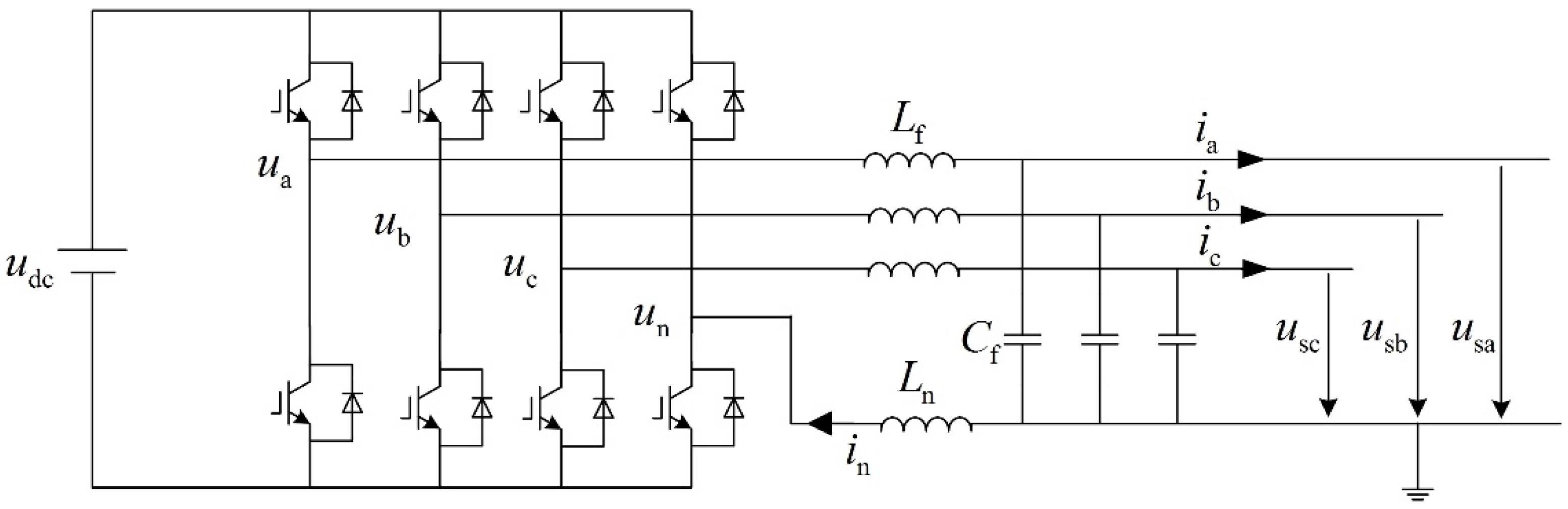
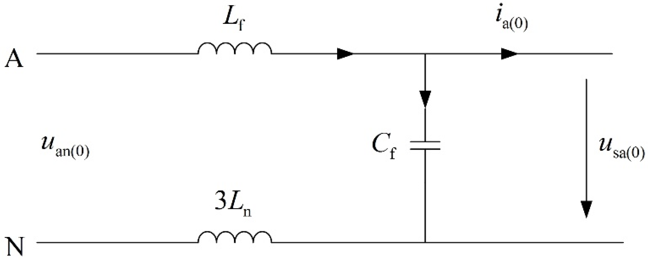
2.1. Modeling and Analysis of the Three-Phase Four-Leg Inverter

Compared with the traditional three-phase inverter, the three-phase four-leg inverter has an extra bridge arm as the neutral point, shown as Figure 1.

In Figure 1, $u_{\mathrm{dc}}$ is the DC voltage, $u_{\mathrm{a}}$, $u_{\mathrm{b}}$, $u_{\mathrm{c}}$, $u_{\mathrm{n}}$ each represent a leg voltage, $i_{\mathrm{n}}$ is the current flowing through the neutral inductor $L_{\mathrm{n}}$, $u_{\mathrm{sa}}$, $u_{\mathrm{sb}}$, $u_{\mathrm{sc}}$ are respectively the voltages of the three phases at the point of common coupling (PCC), and $i_{\mathrm{a}}$, $i_{\mathrm{b}}$, $i_{\mathrm{c}}$ are the currents flowing into PCC. $L_{\mathrm{f}}$ is the three-phase inductance of filter and $C_{\mathrm{f}}$ is the filter capacitance.

It is shown in Figure 1 that the fourth leg can provide a pathway for zero-sequence current. According to the topological structure, the differential equation of the circuit can be written as

$$\begin{array}{l}{u}_{\mathrm{a}}=L_{\mathrm{f}}(\frac{d{i}_{\mathrm{a}}}{dt}+C_{\mathrm{f}}\frac{d^2{u}_{\mathrm{sa}}}{d{t}^2})+u_{\mathrm{sa}}\\ u_{\mathrm{b}}=L_{\mathrm{f}}(\frac{d{i}_{\mathrm{b}}}{dt}+C_{\mathrm{f}}\frac{d^2{u}_{\mathrm{sb}}}{d{t}^2})+u_{\mathrm{sb}}\\ u_{\mathrm{c}}=L_{\mathrm{f}}(\frac{d{i}_{\mathrm{c}}}{dt}+C_{\mathrm{f}}\frac{d^2{u}_{\mathrm{sc}}}{d{t}^2})+u_{\mathrm{sc}}\\ u_{\mathrm{n}}=-L_{\mathrm{n}}\frac{d{i}_{\mathrm{n}}}{dt}\end{array}$$

(1)

Since most of the high-frequency harmonic components of the output voltage and current can be filtered by the grid-connected filter, they are not discussed for the basic control strategy study in this paper. The following analyses are based on fundamental components of 50 or 60 Hz.

To achieve the decoupling of each sequence component with the symmetrical component method, (1) is transformed to the phasor Equation (2).

$$\left[\begin{array}{c}{\dot{U}}_{\mathrm{a}}\\ {\dot{U}}_{\mathrm{b}}\\ {\dot{U}}_{\mathrm{c}}\end{array}\right]=\mathrm{j}\mathsf{\omega }{L}_{\mathrm{f}}\left[\begin{array}{c}{\dot{I}}_{\mathrm{a}}\\ {\dot{I}}_{\mathrm{b}}\\ {\dot{I}}_{\mathrm{c}}\end{array}\right]+(1-{\mathsf{\omega }}^2{L}_{\mathrm{f}}{C}_{\mathrm{f}})\left[\begin{array}{c}{\dot{U}}_{\mathrm{sa}}\\ {\dot{U}}_{\mathrm{sb}}\\ {\dot{U}}_{\mathrm{sc}}\end{array}\right]$$

(2)

Multiplying (2) by the symmetrical component transformation matrix $S$, we get

$$S\left[\begin{array}{c}{\dot{U}}_{\mathrm{a}}\\ {\dot{U}}_{\mathrm{b}}\\ {\dot{U}}_{\mathrm{c}}\end{array}\right]=\mathrm{j}\mathsf{\omega }{L}_{\mathrm{f}}S\left[\begin{array}{c}{\dot{I}}_{\mathrm{a}}\\ {\dot{I}}_{\mathrm{b}}\\ {\dot{I}}_{\mathrm{c}}\end{array}\right]+(1-{\mathsf{\omega }}^2{L}_{\mathrm{f}}{C}_{\mathrm{f}})S\left[\begin{array}{c}{\dot{U}}_{\mathrm{sa}}\\ {\dot{U}}_{\mathrm{sb}}\\ {\dot{U}}_{\mathrm{sc}}\end{array}\right]$$

(3)

where the matrix $S$ is

$$S=\frac{1}{3}\left[\begin{array}{ccc}1& a& a^2\\ 1& a^2& a\\ 1& 1& 1\end{array}\right]$$

(4)

where the operator $a=e^{j{120}^{\circ }}$.

Then there is

$$\left[\begin{array}{c}{\dot{U}}_{\mathrm{a}\left(1\right)}\\ {\dot{U}}_{\mathrm{a}\left(2\right)}\\ {\dot{U}}_{\mathrm{a}\left(0\right)}\end{array}\right]=\mathrm{j}\mathsf{\omega }{L}_{\mathrm{f}}\left[\begin{array}{c}{\dot{I}}_{\mathrm{a}\left(1\right)}\\ {\dot{I}}_{\mathrm{a}\left(2\right)}\\ {\dot{I}}_{\mathrm{a}\left(0\right)}\end{array}\right]+(1-{\mathsf{\omega }}^2{L}_{\mathrm{f}}{C}_{\mathrm{f}})\left[\begin{array}{c}{\dot{U}}_{\mathrm{sa}\left(1\right)}\\ {\dot{U}}_{\mathrm{sa}\left(2\right)}\\ {\dot{U}}_{\mathrm{sa}\left(0\right)}\end{array}\right]$$

(5)

It can be seen from (5) that the three-sequence components are independent of each other, so the differential equations of each sequence in time domain are

$$\begin{array}{l}{u}_{\mathrm{a}(1)}=L_{\mathrm{f}}(\frac{d{i}_{\mathrm{a}(1)}}{dt}+C_{\mathrm{f}}\frac{d^2{u}_{\mathrm{sa}(1)}}{d{t}^2})+u_{\mathrm{sa}(1)}\\ u_{\mathrm{b}(1)}=L_{\mathrm{f}}(\frac{d{i}_{\mathrm{b}(1)}}{dt}+C_{\mathrm{f}}\frac{d^2{u}_{\mathrm{sb}(1)}}{d{t}^2})+u_{\mathrm{sb}(1)}\\ u_{\mathrm{c}(1)}=L_{\mathrm{f}}(\frac{d{i}_{\mathrm{c}(1)}}{dt}+C_{\mathrm{f}}\frac{d^2{u}_{\mathrm{sc}(1)}}{d{t}^2})+u_{\mathrm{sc}(1)}\end{array}$$

(6)

$$\begin{array}{l}{u}_{\mathrm{a}(2)}=L_{\mathrm{f}}(\frac{d{i}_{\mathrm{a}(2)}}{dt}+C_{\mathrm{f}}\frac{d^2{u}_{\mathrm{sa}(2)}}{d{t}^2})+u_{\mathrm{sa}(2)}\\ u_{\mathrm{b}(2)}=L_{\mathrm{f}}(\frac{d{i}_{\mathrm{b}(2)}}{dt}+C_{\mathrm{f}}\frac{d^2{u}_{\mathrm{sb}(2)}}{d{t}^2})+u_{\mathrm{sb}(2)}\\ u_{\mathrm{c}(2)}=L_{\mathrm{f}}(\frac{d{i}_{\mathrm{c}(2)}}{dt}+C_{\mathrm{f}}\frac{d^2{u}_{\mathrm{sc}(2)}}{d{t}^2})+u_{\mathrm{sc}(2)}\end{array}$$

(7)

$$u_{\mathrm{a}\left(0\right)}=L_{\mathrm{f}}(\frac{d{i}_{\mathrm{a}(0)}}{dt}+C_{\mathrm{f}}\frac{d^2{u}_{\mathrm{sa}(0)}}{d{t}^2})+u_{\mathrm{sa}(0)}$$

(8)

Subscripts ₍₁₎, ₍₂₎, and ₍₀₎ respectively indicate the positive, negative and zero sequence components. Then (6) is the positive sequence equation of the inverter, while (7) is the negative and (8) is the zero. As the zero sequence components of three phases are exactly identical, only the equation of phase A is given.

According to the Kirchhoff’s Current Law, the current $i_{\mathrm{n}}$ flowing through the neutral line must satisfy

$$i_{\mathrm{n}}=(i_{\mathrm{a}}+i_{\mathrm{b}}+i_{\mathrm{c}})+C_{\mathrm{f}}(\frac{d{u}_{\mathrm{sa}}}{dt}+\frac{d{u}_{\mathrm{sb}}}{dt}+\frac{d{u}_{\mathrm{sc}}}{dt})=3(i_{\mathrm{a}(0)}+C_{\mathrm{f}}\frac{d{u}_{\mathrm{sa}(0)}}{dt})$$

(9)

So, the fourth equation in (1) can be written as

$$u_{\mathrm{n}}=-3L_{\mathrm{n}}(\frac{d{i}_{\mathrm{a}(0)}}{dt}+C_{\mathrm{f}}\frac{d^2{u}_{\mathrm{sa}(0)}}{d{t}^2})$$

(10)

From (9) and (10) we can know that the neutral line current $i_{\mathrm{n}}$ only contains the zero sequence component. Therefore, the output voltage of the fourth leg is just the zero sequence voltage.

Through the analysis, it is known that the positive and negative sequence components are only dependent on the voltages and currents of the first three legs, consistent with the mathematical model of the traditional three-phase inverter, but the zero sequence components are different.

According to (8) and (10), the zero sequence equation is

$$u_{\mathrm{an}(0)}=u_{\mathrm{a}(0)}-u_{\mathrm{n}}=(L_{\mathrm{f}}+3L_{\mathrm{n}})(\frac{d{i}_{\mathrm{a}(0)}}{dt}+C_{\mathrm{f}}\frac{d^2{u}_{\mathrm{sa}(0)}}{d{t}^2})+u_{\mathrm{sa}(0)}$$

(11)

where $u_{\mathrm{an}(0)}$ is the zero sequence potential difference between the outlets of the first and fourth legs.

The zero sequence circuit topology described by (11) is shown in Figure 2.

In summary, (6), (7), and (11) can respectively describe the positive, negative, and zero sequence mathematical models of three-phase four leg inverter. To maintain the symmetry of the three-phase voltage in the low-voltage distribution network with unbalanced loads, the negative and zero sequence voltage have to be 0. In other words, the PCC voltage contains only the positive sequence component.

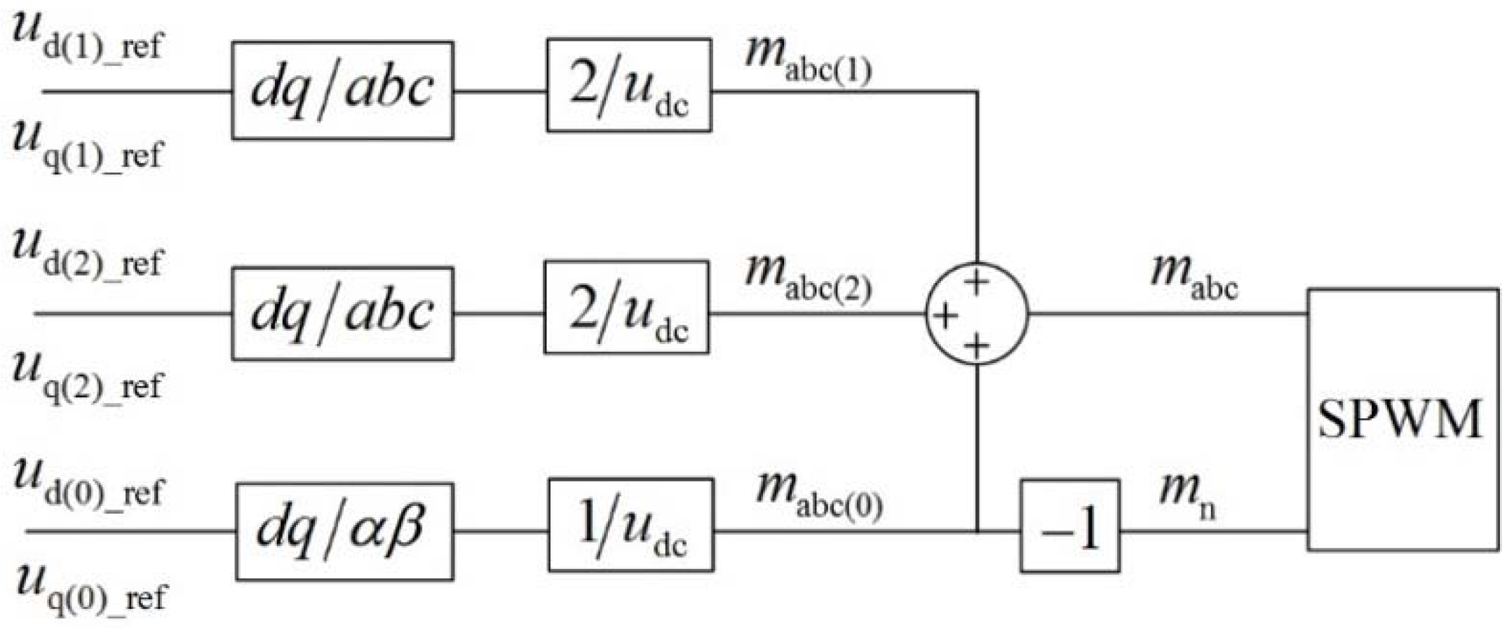
2.2. Control Strategy of Positive and Negative Sequence Components

For the grid-connected distributed generator (DG), the constant power control (PQ control) is widely adopted. According to the instantaneous power theory [23], the average part of instantaneous power, in which form the energy is transferred in the three-phase four-wire system, can be expressed as (12).

$$\begin{array}{l}\overline{p}=3V_{\left(1\right)}{I}_{\left(1\right)}\cos {\varphi }_{v\left(1\right)}-{\varphi }_{i\left(1\right)})+3V_{\left(2\right)}{I}_{\left(2\right)}\cos {\varphi }_{v\left(2\right)}-{\varphi }_{i\left(2\right)})+3V_{\left(0\right)}{I}_{\left(0\right)}\cos {\varphi }_{v\left(0\right)}-{\varphi }_{i\left(0\right)})\\ \overline{q}=3V_{\left(1\right)}{I}_{\left(1\right)}\sin {\varphi }_{v\left(1\right)}-{\varphi }_{i\left(1\right)})-3V_{\left(2\right)}{I}_{\left(2\right)}\sin {\varphi }_{v\left(2\right)}-{\varphi }_{i\left(2\right)})\end{array}$$

(12)

where $\overline{p}$, $\overline{q}$ represent the average parts of active power and reactive power respectively, and the pairs of $V_{\left(1\right)}$ and $I_{\left(1\right)}$, $V_{\left(2\right)}$ and $I_{\left(2\right)}$, as well as $V_{\left(0\right)}$ and $I_{\left(0\right)}$, represent the effective voltage and current values of positive, negative and zero sequences separately, with their corresponding phases being ${\varphi }_{v\left(1\right)}$, ${\varphi }_{i\left(1\right)}$, ${\varphi }_{v\left(2\right)}$, ${\varphi }_{i\left(2\right)}$, ${\varphi }_{v\left(0\right)}$, and ${\varphi }_{i\left(0\right)}$.

Assuming the negative and zero sequence voltages are 0 to achieve symmetry, $\overline{p}$ and $\overline{q}$ in (12) are determined only by the positive sequence components. Therefore, the positive sequence components can be regulated with the PQ control method as a way to control the power flow.

Through the Park transformation, both the positive sequence and the negative sequence components acquire the DC form in d-q coordinate system, and thus can be easily controlled by the PI controller without the static error [24]. Here we show the transforming process:

The Park transformation matrix is

$$C_{3\mathrm{s}/2\mathrm{r}}=\frac{2}{3}\left[\begin{array}{l}\begin{array}{ccc}\cos \mathsf{\theta }& \cos (\mathsf{\theta }-\frac{2\mathsf{\pi }}{3})& \cos (\mathsf{\theta }+\frac{2\mathsf{\pi }}{3})\end{array}\\ \begin{array}{ccc}-\sin \mathsf{\theta }& -\sin (\mathsf{\theta }-\frac{2\mathsf{\pi }}{3})& -\sin (\mathsf{\theta }+\frac{2\mathsf{\pi }}{3})\end{array}\end{array}\right]$$

(13)

For the positive sequence,

$$\left[\begin{array}{c}{u}_{\mathrm{sd}\left(1\right)}\\ u_{\mathrm{sq}\left(1\right)}\end{array}\right]=C_{3\mathrm{s}/2\mathrm{r}}\left[\begin{array}{c}{u}_{\mathrm{sa}\left(1\right)}\\ u_{\mathrm{sb}\left(1\right)}\\ u_{\mathrm{sc}\left(1\right)}\end{array}\right]=C_{3\mathrm{s}/2\mathrm{r}}\left[\begin{array}{c}{U}_{\left(1\right)\mathrm{m}}\sin (\mathsf{\omega }t+{\mathsf{\alpha }}_1)\\ U_{\left(1\right)\mathrm{m}}\sin (\mathsf{\omega }t+{\mathsf{\alpha }}_1-2\mathsf{\pi }/3)\\ U_{\left(1\right)\mathrm{m}}\sin (\mathsf{\omega }t+{\mathsf{\alpha }}_1+2\mathsf{\pi }/3)\end{array}\right]=U_{\left(1\right)\mathrm{m}}\left[\begin{array}{c}\sin (\mathsf{\omega }t+{\mathsf{\alpha }}_1-\mathsf{\theta })\\ -\cos (\mathsf{\omega }t+{\mathsf{\alpha }}_1-\mathsf{\theta })\end{array}\right]$$

(14)

where $u_{\mathrm{sd}\left(1\right)}$ and $u_{\mathrm{sq}\left(1\right)}$ are the d-axis and q-axis components of the PCC positive voltage, $U_{\left(1\right)\mathrm{m}}$ is its amplitude and $\mathsf{\omega }$ is the system angular frequency which is obtained by the phase-locked loop (PLL) in real time, and ${\mathsf{\alpha }}_1$ is the initial phase of $u_{\mathrm{sa}\left(1\right)}$. To make $u_{\mathrm{sd}\left(1\right)}$ and $u_{\mathrm{sq}\left(1\right)}$ take the DC form, and to enable $u_{\mathrm{sq}\left(1\right)}=0$, the following condition has to be met

$$\mathsf{\theta }=\mathsf{\omega }t+{\mathsf{\alpha }}_1-\mathsf{\pi }/2$$

(15)

For the negative sequence, the negative sequence current is used as an example. Let ${\mathsf{\theta }}^{\prime }=-\mathsf{\theta }=-(\mathsf{\omega }t+{\mathsf{\alpha }}_1-\mathsf{\pi }/2)$, and get $C_{3\mathrm{s}/2\mathrm{r}}^{\prime }$ by replacing the $\mathsf{\theta }$ in $C_{3\mathrm{s}/2\mathrm{r}}$ with ${\mathsf{\theta }}^{\prime }$. Then,

$$\left[\begin{array}{c}{i}_{\mathrm{d}\left(2\right)}\\ i_{\mathrm{q}\left(2\right)}\end{array}\right]=C_{3\mathrm{s}/2\mathrm{r}}^{\prime }\left[\begin{array}{c}{i}_{\mathrm{a}\left(2\right)}\\ i_{\mathrm{b}\left(2\right)}\\ i_{\mathrm{c}\left(2\right)}\end{array}\right]=C_{3\mathrm{s}/2\mathrm{r}}^{\prime }\left[\begin{array}{c}{I}_{\left(2\right)\mathrm{m}}\sin (\mathsf{\omega }t+{\mathsf{\phi }}_2)\\ I_{\left(2\right)\mathrm{m}}\sin (\mathsf{\omega }t+{\mathsf{\phi }}_2+2\mathsf{\pi }/3)\\ I_{\left(2\right)\mathrm{m}}\sin (\mathsf{\omega }t+{\mathsf{\phi }}_2-2\mathsf{\pi }/3)\end{array}\right]=I_{\left(2\right)\mathrm{m}}\left[\begin{array}{c}\cos ({\mathsf{\phi }}_2-{\mathsf{\alpha }}_1)\\ -\sin ({\mathsf{\phi }}_2-{\mathsf{\alpha }}_1)\end{array}\right]$$

(16)

where $I_{\left(2\right)\mathrm{m}}$ and ${\mathsf{\phi }}_2$ are the amplitude and initial phase of $i_{\mathrm{a}\left(2\right)}$.

Through the transformations (14) and (16), the PI controller is introduced to the d-q frame. Because the harmonics in the primary currents and voltages will bring problems for PI controller, low pass filters should be applied to the decomposition process of sequence components.

The inner-loop and outer-loop controllers of the positive sequence components are expressed as (17) and (18), respectively.

$$\begin{array}{l}{u}_{\mathrm{d}\left(1\right)\_\mathrm{ref}}=(K_{\mathrm{iP}\left(1\right)}+\frac{K_{\mathrm{iI}\left(1\right)}}{s})(i_{\mathrm{d}\left(1\right)\_\mathrm{ref}}-i_{\mathrm{d}\left(1\right)})-\mathsf{\omega }{L}_{\mathrm{f}}{i}_{\mathrm{q}\left(1\right)}+u_{\mathrm{sd}\left(1\right)}\\ u_{\mathrm{q}\left(1\right)\_\mathrm{ref}}=(K_{\mathrm{iP}\left(1\right)}+\frac{K_{\mathrm{iI}\left(1\right)}}{s})(i_{\mathrm{q}\left(1\right)\_\mathrm{ref}}-i_{\mathrm{q}\left(1\right)})+\mathsf{\omega }{L}_{\mathrm{f}}{i}_{\mathrm{d}\left(1\right)}+u_{\mathrm{sq}\left(1\right)}\end{array}$$

(17)

$$\begin{array}{l}{i}_{\mathrm{d}\left(1\right)\_\mathrm{ref}}=(K_{\mathrm{oP}\left(1\right)}+\frac{K_{\mathrm{oI}\left(1\right)}}{s})(P_{\mathrm{ref}}-P)\\ i_{\mathrm{q}\left(1\right)\_\mathrm{ref}}=(K_{\mathrm{oP}\left(1\right)}+\frac{K_{\mathrm{oI}\left(1\right)}}{s})(Q_{\mathrm{ref}}-Q)\end{array}$$

(18)

where $i_{\mathrm{d}\left(1\right)}$ and $i_{\mathrm{q}\left(1\right)}$ are the d-axis and q-axis components of the positive sequence current; $K_{\mathrm{iP}\left(1\right)}$ and $K_{\mathrm{oP}\left(1\right)}$ the proportionality coefficients of the inner and outer loops; $K_{\mathrm{iI}\left(1\right)}$ and $K_{\mathrm{oI}\left(1\right)}$ the integral coefficients of the inner and outer loops; $i_{\mathrm{d}\left(1\right)\_\mathrm{ref}}$ and $i_{\mathrm{q}\left(1\right)\_\mathrm{ref}}$ the reference currents; $P_{\mathrm{ref}}$ and $Q_{\mathrm{ref}}$ the reference powers; and, $u_{\mathrm{d}\left(1\right)\_\mathrm{ref}}$ and $u_{\mathrm{q}\left(1\right)\_\mathrm{ref}}$ the modulation signals.

The outer loop is used to achieve power control, while the inner loop speeds up the dynamic response.

For the negative sequence components, as they are converted to the DC form, they can also be regulated by the same control method as the positive sequence components in (17) and (18), with components $P$ and $Q$ replaced by the negative voltages for the outer loop control [25]:

$$\begin{array}{l}{i}_{\mathrm{d}\left(2\right)\_\mathrm{ref}}=-(K_{\mathrm{oP}\left(2\right)}+\frac{K_{\mathrm{oI}\left(2\right)}}{s})u_{\mathrm{sd}\left(2\right)}\\ i_{\mathrm{q}\left(2\right)\_\mathrm{ref}}=-(K_{\mathrm{oP}\left(2\right)}+\frac{K_{\mathrm{oI}\left(2\right)}}{s})u_{\mathrm{sq}\left(2\right)}\end{array}$$

(19)

The positive and negative sequence control strategies are illustrated in Figure 3.

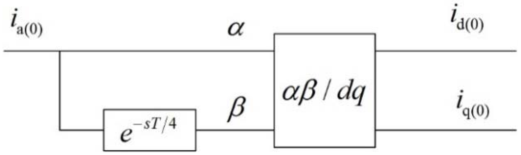
2.3. Control Strategy of Zero Sequence Component

In (11), the zero sequence model of the three-phase four-leg inverter can be regarded as a single-phase inverter, so it can be controlled by a similar strategy to that of a single-phase inverter.

Due to the static error in controlling an AC system, the PI controller fails when high precision is required, and has to give way to the proportional resonant (PR) controller, which has no static error. However, this is only in principle, for it is difficult to build an ideal PR controller and its regulating performance is subject to the fluctuations of the grid frequency [26]. Another way to avoid this disadvantage is trying to convert the single-phase AC signal to DC form to make it acceptable for the application of the PI controller.

For a single-phase voltage or current, with a delay of a quarter of the period, a new signal is created, whose vector is perpendicular to that of the former [27]. The two signals can be converted into DC components through the αβ-dq transformation. Take the zero sequence current $i_{\mathrm{a}\left(0\right)}$ for example, whose expression is

$$i_{\mathrm{a}\left(0\right)}=I_{\left(0\right)\mathrm{m}}\sin (\mathsf{\omega }t+{\mathsf{\phi }}_0)$$

(20)

In the αβ static coordinate system, let

$$\begin{array}{l}{i}_{\mathsf{\alpha }}=i_{\mathrm{a}\left(0\right)}=I_{\left(0\right)\mathrm{m}}\sin (\mathsf{\omega }t+{\mathsf{\phi }}_0)\\ i_{\mathsf{\beta }}=I_{\left(0\right)\mathrm{m}}\sin (\mathsf{\omega }t+{\mathsf{\phi }}_0-{90}^{\circ })=-I_{\left(0\right)\mathrm{m}}\cos (\mathsf{\omega }t+{\mathsf{\phi }}_0)\end{array}$$

(21)

After the αβ-dq transformation, two DC components $i_{\mathrm{d}\left(0\right)}$ and $i_{\mathrm{q}\left(0\right)}$ are obtained as

$$\left[\begin{array}{c}{i}_{\mathrm{d}\left(0\right)}\\ i_{\mathrm{q}\left(0\right)}\end{array}\right]=\left[\begin{array}{cc}\cos \mathsf{\theta }& \sin \mathsf{\theta }\\ -\sin \mathsf{\theta }& \cos \mathsf{\theta }\end{array}\right]\left[\begin{array}{c}{i}_{\mathsf{\alpha }}\\ i_{\mathsf{\beta }}\end{array}\right]=I_{\left(0\right)\mathrm{m}}\left[\begin{array}{c}\sin (\mathsf{\omega }t+{\mathsf{\phi }}_0-\mathsf{\theta })\\ -\cos (\mathsf{\omega }t+{\mathsf{\phi }}_0-\mathsf{\theta })\end{array}\right]=I_{\left(0\right)\mathrm{m}}\left[\begin{array}{c}\cos ({\mathsf{\phi }}_0-{\mathsf{\alpha }}_1)\\ \sin ({\mathsf{\phi }}_0-{\mathsf{\alpha }}_1)\end{array}\right]$$

(22)

where $\mathsf{\theta }=\mathsf{\omega }t+{\mathsf{\alpha }}_1-\mathsf{\pi }/2$.

Figure 4 illustrates the transformation process.

Through the transformation, the static error of the PI controller can be eliminated. The control method is similar to that of negative sequence components, only with $L_{\mathrm{f}}$ replaced by $(L_{\mathrm{f}}+3L_{\mathrm{n}})$ and each voltage and current replaced by its zero sequence counterpart in (17) and (19).

Finally, the control signals of the three sequences should be superimposed and modulated in the way shown in Figure 5 to achieve the control on the three-phase four-leg inverter. In this paper, sine-wave pulse-width modulation (SPWM) is chosen as the modulation strategy.

3. Current-Limiting Scheme Embedded in Control Strategy

To maintain the PCC voltage symmetry, each phase current output by the three-phase four-leg inverter is usually unequal in magnitude with others. The method of the modulus limit on current reference value is not applicable to limiting the output current and protect the inverter. In addition, setting limit values for each sequence independently may cause the waste of the inverter capacity. It is necessary to find a method which can limit the phase currents and make full use of the capacity of the inverter.

According to the control strategy above, the controller of each sequence is independent with others. The positive sequence current is determined by the target of the output power. It takes on the role of outputting active and reactive power. The negative and zero sequence currents depend on the load condition, and they play a common role of balancing the PCC voltage. Thus, the negative and zero sequence currents can be put into one block to be discussed, and for convenience, their sum ${\dot{I}}_{\mathrm{k}(2,0)}$ can be called as the balance regulating current.

$${\dot{I}}_{\mathrm{k}(2,0)}={\dot{I}}_{\mathrm{k}\left(2\right)}+{\dot{I}}_{\left(0\right)},(\mathrm{k}=\mathrm{a},\mathrm{b},\mathrm{c})$$

(23)

where ${\dot{I}}_{\mathrm{k}\left(2\right)}$ is the negative sequence current of phase k, and as the zero sequence components of three phases are exactly identical, the zero sequence current is written as ${\dot{I}}_{\left(0\right)}$.

Then, the currents are divided into two categories: the positive sequence current is for power transmission, and the balance regulating current, which is the sum of the negative and zero sequence currents, is for voltage balance.

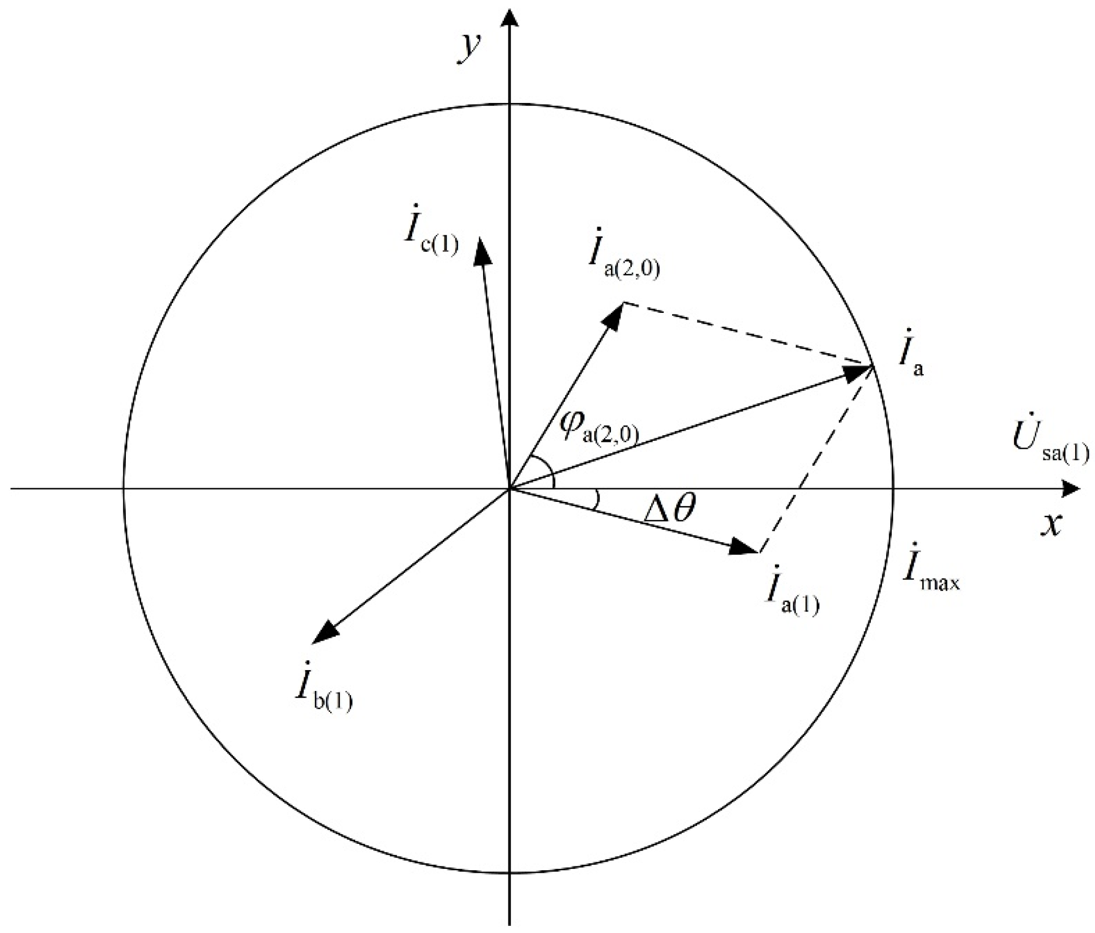
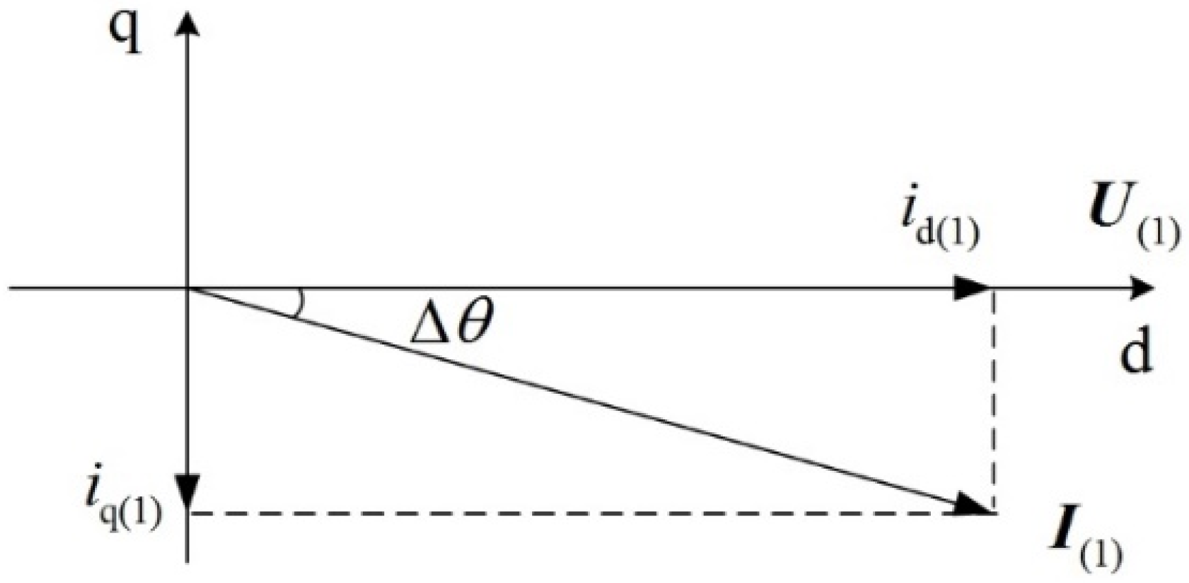
3.1. Output Characteristic of Each Sequence

When the direction of the AC voltage vector $U_{\left(1\right)}$ is selected as that of the d-axis in the synchronous rotating coordinate system, the output power and positive sequence current of the DG have such relationships [24]

$$\{\begin{array}{c}P=1.5u_{\mathrm{sd}\left(1\right)}{i}_{\mathrm{d}\left(1\right)}\\ Q=-1.5u_{\mathrm{sd}\left(1\right)}{i}_{\mathrm{q}\left(1\right)}\end{array}$$

(24)

where $P$ and $Q$ are the active power and reactive power output by the inverter. Since the Park transformation will not change the amplitude, $u_{\mathrm{sd}\left(1\right)}$ has the same amplitude with $U_{\left(1\right)}$.

Therefore, the d-axis and q-axis components of the positive sequence current can be obtained as

$$\{\begin{array}{c}{i}_{\mathrm{d}\left(1\right)}=\frac{2}{3}\frac{P}{u_{\mathrm{sd}\left(1\right)}}=\frac{2}{3}\frac{P}{\left|U_{\left(1\right)}\right|}\\ i_{\mathrm{q}\left(1\right)}=-\frac{2}{3}\frac{Q}{u_{\mathrm{sd}\left(1\right)}}=-\frac{2}{3}\frac{Q}{\left|U_{\left(1\right)}\right|}\end{array}$$

(25)

According to Figure 6, the current vector $I_{(1)}$ lags behind the voltage vector $U_{\left(1\right)}$ by an angle $\Delta \mathsf{\theta }$. Accordingly, each phase current lags behind the corresponding phase voltage by $\Delta \mathsf{\theta }$ in abc frame. According to (14), the amplitude of each phase current is equal with that of $I_{(1)}$. The A phase current phasor can be expressed as

$${\dot{I}}_{\mathrm{a}\left(1\right)}=\sqrt{i_{\mathrm{d}\left(1\right)}^2+i_{\mathrm{q}\left(1\right)}^2}\angle ({\mathsf{\theta }}_0+\Delta \mathsf{\theta })$$

(26)

where ${\mathsf{\theta }}_0=\arg {\dot{U}}_{\mathrm{sa}\left(1\right)}$ and $\Delta \mathsf{\theta }=\arctan (i_{\mathrm{q}\left(1\right)}/i_{\mathrm{d}\left(1\right)})$.

In addition, the control system of the inverter is generally equipped with a modulus limiter, which can limit the amplitude of the output current within a certain value $I_{\left(1\right)\max }$. Therefore, according to (25) and (26), the positive sequence current is

$${\dot{I}}_{\mathrm{a}\left(1\right)}=\frac{2}{3}\frac{\sqrt{{P_{\mathrm{ref}}}^2+{Q_{\mathrm{ref}}}^2}}{\left|U_{\left(1\right)}\right|}\angle ({\mathsf{\theta }}_0+\Delta \mathsf{\theta }),\frac{2}{3}\frac{\sqrt{{P_{\mathrm{ref}}}^2+{Q_{\mathrm{ref}}}^2}}{\left|U_{\left(1\right)}\right|}<I_{(1)\max }$$

(27)

When the voltage is very small, which means the ${\dot{I}}_{\mathrm{a}\left(1\right)}$ will be rather large, ${\dot{I}}_{\mathrm{a}\left(1\right)}$ should be limited at the maximum value $I_{\left(1\right)\max }$. The modulus limiter can limit the amplitude of the current without changing its phase [25]. Then, the positive sequence current can be written as

$${\dot{I}}_{\mathrm{a}\left(1\right)}=I_{\left(1\right)\max }\angle ({\mathsf{\theta }}_0+\Delta \mathsf{\theta }),\frac{2}{3}\frac{\sqrt{{P_{\mathrm{ref}}}^2+{Q_{\mathrm{ref}}}^2}}{\left|U_{\left(1\right)}\right|}\ge I_{(1)\max }$$

(28)

For the negative and zero sequence currents, which are introduced to maintain voltage symmetry, they are determined by loads, and only the electrical states of the negative and zero sequence components are known

$${\dot{U}}_{\mathrm{sa}\left(2\right)}={\dot{U}}_{\mathrm{s}\left(0\right)}=0,\left|{\dot{I}}_{\mathrm{k}(2,0)}\right|<I_{(2,0)\max }(\mathrm{k}=\mathrm{a},\mathrm{b},\mathrm{c})$$

(29)

where the zero sequence voltage of PCC is written as ${\dot{U}}_{\mathrm{s}\left(0\right)}$ for that of each phase is identical; ${\dot{U}}_{\mathrm{sa}\left(2\right)}$ is the A phase negative voltage and $I_{(2,0)\max }$ is the amplitude limit of the balance regulating current ${\dot{I}}_{\mathrm{k}(2,0)}$.

To keep the voltages of both the negative sequence and zero sequence being zero, the amplitude of ${\dot{I}}_{\mathrm{k}(2,0)}$ cannot exceed $I_{(2,0)\max }$. It is noted that if the amplitude of ${\dot{I}}_{\mathrm{k}(2,0)}$ for any phase has the trend of surpassing $I_{(2,0)\max }$, it will be limited at this maximum, but in this case, the voltages may not be maintained at 0.

$$\max \left|{\dot{I}}_{\mathrm{k}(2,0)}\right|=I_{(2,0)\max }(\mathrm{k}=\mathrm{a},\mathrm{b},\mathrm{c})$$

(30)

Thus $I_{(2,0)\max }$ can be seen as an indicator of the capability of the inverter to maintain the voltage symmetry.

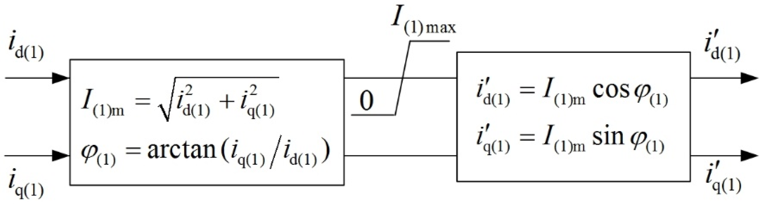
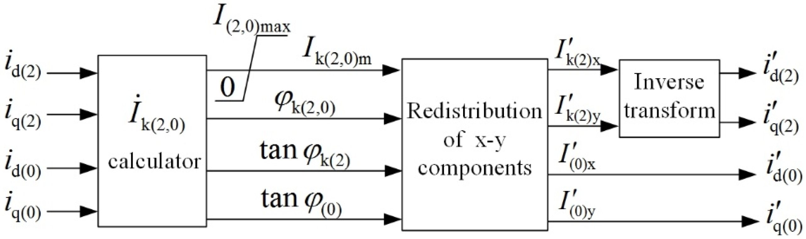
3.2. Current Modulus Limiters of Each Sequence

The equations in (28) and (30) can be satisfied by applying a modulus limiter to each of the outer loops.

For (28), the three-phase current is symmetrical, so the model of the modulus limiter in Figure 7 can be used [24].

However, for (30), the balance regulating current ${\dot{I}}_{\mathrm{k}(2,0)}$ of each phase is unique and thus should be calculated separately.

For the negative and zero sequence currents, after the Park transformation, the d-axis and q-axis components are shown as (16) and (22) respectively.

Then make the phasor diagram of the negative and zero sequence currents as Figure 8. By selecting the direction of ${\dot{U}}_{\mathrm{sa}\left(1\right)}$ as that of the x-axis, a Rectangular coordinate system is built, where the x-axis and y-axis components of each phase can be obtained.

In terms of the negative sequence, the components of the three phases are calculated according to the Figure 8 and Park transformation results (16) and (22).

For phase A,

$$\begin{array}{l}{I}_{\mathrm{a}\left(2\right)\mathrm{x}}=I_{\left(2\right)\mathrm{m}}\cos ({\mathsf{\phi }}_2-{\mathsf{\alpha }}_1)=i_{\mathrm{d}\left(2\right)}\\ I_{\mathrm{a}\left(2\right)\mathrm{y}}=I_{\left(2\right)\mathrm{m}}\sin ({\mathsf{\phi }}_2-{\mathsf{\alpha }}_1)=-i_{\mathrm{q}\left(2\right)}\end{array}$$

(31)

For phase B,

$$\begin{array}{l}{I}_{\mathrm{b}\left(2\right)\mathrm{x}}=I_{\left(2\right)\mathrm{m}}\cos ({\mathsf{\phi }}_2-{\mathsf{\alpha }}_1+\frac{2\mathsf{\pi }}{3})=-\frac{1}{2}{i}_{\mathrm{d}\left(2\right)}+\frac{\sqrt{3}}{2}{i}_{\mathrm{q}\left(2\right)}\\ I_{\mathrm{b}\left(2\right)\mathrm{y}}=I_{\left(2\right)\mathrm{m}}\sin ({\mathsf{\phi }}_2-{\mathsf{\alpha }}_1+\frac{2\mathsf{\pi }}{3})=\frac{\sqrt{3}}{2}{i}_{\mathrm{d}\left(2\right)}+\frac{1}{2}{i}_{\mathrm{q}\left(2\right)}\end{array}$$

(32)

For phase C,

$$\begin{array}{l}{I}_{\mathrm{c}\left(2\right)\mathrm{x}}=I_{\left(2\right)\mathrm{m}}\cos ({\mathsf{\phi }}_2-{\mathsf{\alpha }}_1-\frac{2\mathsf{\pi }}{3})=-\frac{1}{2}{i}_{\mathrm{d}\left(2\right)}-\frac{\sqrt{3}}{2}{i}_{\mathrm{q}\left(2\right)}\\ I_{\mathrm{c}\left(2\right)\mathrm{y}}=I_{\left(2\right)\mathrm{m}}\sin ({\mathsf{\phi }}_2-{\mathsf{\alpha }}_1-\frac{2\mathsf{\pi }}{3})=-\frac{\sqrt{3}}{2}{i}_{\mathrm{d}\left(2\right)}+\frac{1}{2}{i}_{\mathrm{q}\left(2\right)}\end{array}$$

(33)

In (31), (32), and (33), $I_{\mathrm{k}\left(2\right)\mathrm{x}}$ and $I_{\mathrm{k}\left(2\right)\mathrm{y}}$ (k = a, b, c) are the x-axis and y-axis components of the negative sequence current of phase k, and ${\phi }_2$ the phase angle of ${\dot{I}}_{\mathrm{a}\left(2\right)}$.

For the zero sequence current,

$$\begin{array}{l}{I}_{\left(0\right)\mathrm{x}}=I_{\left(0\right)\mathrm{m}}\cos ({\mathsf{\phi }}_0-{\mathsf{\alpha }}_1)=i_{\mathrm{d}\left(0\right)}\\ I_{\left(0\right)\mathrm{y}}=I_{\left(0\right)\mathrm{m}}\sin ({\mathsf{\phi }}_0-{\mathsf{\alpha }}_1)=i_{\mathrm{q}\left(0\right)}\end{array}$$

(34)

Therefore, the balance regulating current ${\dot{I}}_{\mathrm{k}(2,0)}$ can be calculated through (35).

$$\begin{array}{l}{I}_{\mathrm{k}(2,0)\mathrm{m}}=\sqrt{{(I_{\mathrm{k}\left(2\right)\mathrm{x}}+I_{\left(0\right)\mathrm{x}})}^2+{(I_{\mathrm{k}\left(2\right)\mathrm{y}}+I_{\left(0\right)\mathrm{y}})}^2}\\ \tan {\mathsf{\phi }}_{\mathrm{k}(2,0)}=\frac{I_{\mathrm{k}\left(2\right)\mathrm{y}}+I_{\left(0\right)\mathrm{y}}}{I_{\mathrm{k}\left(2\right)\mathrm{x}}+I_{\left(0\right)\mathrm{x}}}\end{array}$$

(35)

where $I_{\mathrm{k}(2,0)\mathrm{m}}$ is the amplitude of ${\dot{I}}_{\mathrm{k}(2,0)}$; ${\phi }_{\mathrm{k}(2,0)}$ the included angle between ${\dot{I}}_{\mathrm{k}(2,0)}$ and the x-axis; $I_{\left(0\right)\mathrm{x}}$ and $I_{\left(0\right)\mathrm{y}}$ the x-axis and y-axis components of the zero sequence current.

The modulus limit for ${\dot{I}}_{\mathrm{k}(2,0)}$ can be achieved by the limiter in Figure 9.

In Figure 9, ${\mathsf{\phi }}_{\mathrm{k}\left(2\right)}$ is the included angle between ${\dot{I}}_{\mathrm{k}\left(2\right)}$ and the x-axis, and ${\mathsf{\phi }}_{\left(0\right)}$ is that between ${\dot{I}}_{\left(0\right)}$ and the x-axis, which can be deduced by

$$\begin{array}{l}\tan {\mathsf{\phi }}_{\mathrm{k}\left(2\right)}=I_{\mathrm{k}\left(2\right)\mathrm{y}}/I_{\mathrm{k}\left(2\right)\mathrm{x}}\\ \tan {\mathsf{\phi }}_{\left(0\right)}=I_{\left(0\right)\mathrm{y}}/I_{\left(0\right)\mathrm{x}}\end{array}$$

(36)

To limit the amplitude of the balance regulating current without changing the phase angle, the redistribution of the x-axis and y-axis components can be achieved by

$$\{\begin{array}{c}{I}_{\mathrm{k}\left(2\right)\mathrm{y}}^{\prime }/I_{\mathrm{k}\left(2\right)\mathrm{x}}^{\prime }=\tan {\mathsf{\phi }}_{\mathrm{k}\left(2\right)}\\ I_{\left(0\right)\mathrm{y}}^{\prime }/I_{\left(0\right)\mathrm{x}}^{\prime }=\tan {\mathsf{\phi }}_{\left(0\right)}\\ I_{\mathrm{k}\left(2\right)\mathrm{x}}^{\prime }+I_{\left(0\right)\mathrm{x}}^{\prime }=I_{\mathrm{k}(2,0)\mathrm{m}}\cos {\mathsf{\phi }}_{\mathrm{k}(2,0)}\\ I_{\mathrm{k}\left(2\right)\mathrm{y}}^{\prime }+I_{\left(0\right)\mathrm{y}}^{\prime }=I_{\mathrm{k}(2,0)\mathrm{m}}\sin {\mathsf{\phi }}_{\mathrm{k}(2,0)}\end{array}$$

(37)

It is defined that

$${\mathsf{\beta }}_{\mathrm{k}}=\frac{I_{\mathrm{k}(2,0)\mathrm{m}}\cos {\mathsf{\phi }}_{\mathrm{k}(2,0)}}{\tan {\mathsf{\phi }}_{(0)}-\tan {\mathsf{\phi }}_{\mathrm{k}\left(2\right)}}$$

(38)

The negative and zero sequence components output by the modulus limiter are

$$\{\begin{array}{c}{I}_{\mathrm{k}\left(2\right)\mathrm{x}}^{\prime }={\mathsf{\beta }}_{\mathrm{k}}(\tan {\mathsf{\phi }}_{\left(0\right)}-\tan {\mathsf{\phi }}_{\mathrm{k}(2,0)})\\ I_{\mathrm{k}\left(2\right)\mathrm{y}}^{\prime }={\mathsf{\beta }}_{\mathrm{k}}(\tan {\mathsf{\phi }}_{\left(0\right)}-\tan {\mathsf{\phi }}_{\mathrm{k}(2,0)})\tan {\mathsf{\phi }}_{\mathrm{k}\left(2\right)}\\ I_{\left(0\right)\mathrm{x}}^{\prime }={\mathsf{\beta }}_{\mathrm{k}}(\tan {\mathsf{\phi }}_{\mathrm{k}(2,0)}-\tan {\mathsf{\phi }}_{\mathrm{k}\left(2\right)})\\ I_{\left(0\right)\mathrm{y}}^{\prime }={\mathsf{\beta }}_{\mathrm{k}}(\tan {\mathsf{\phi }}_{\mathrm{k}(2,0)}-\tan {\mathsf{\phi }}_{\mathrm{k}\left(2\right)})\tan {\mathsf{\phi }}_{\left(0\right)}\end{array}$$

(39)

It is noted that (39) needs to be calculated for each of the three phases separately, and the corresponding $i_{\mathrm{d}\left(2\right)}^{\prime }$, $i_{\mathrm{q}\left(2\right)}^{\prime }$, $i_{\mathrm{d}\left(0\right)}^{\prime }$ and $i_{\mathrm{q}\left(0\right)}^{\prime }$ for each phase can be obtained through the inverse transformation of (31)–(33). The minimum of them will be used as the new references to ensure that each phase current does not exceed the limit value.

3.3. Combined Current-Limiting Method

The amplitude limit value for the positive sequence current is $I_{(1)\max }$, and that for the sum of the negative and zero sequence currents is $I_{(2,0)\max }$, but the real constriction for the inverter output current is the maximum phase current which is determined by the current-carrying capacity of the IGBT and the saturation current of the output filter. Therefore, the real current limit should be modified as

$$\{\begin{array}{c}\left|{\dot{I}}_{\mathrm{k}\left(1\right)}+{\dot{I}}_{\mathrm{k}\left(2\right)}+{\dot{I}}_{\left(0\right)}\right|<I_{\max }\\ 3\left|{\dot{I}}_{\left(0\right)}\right|<I_{\max }\end{array}(\mathrm{k}=\mathrm{a},\mathrm{b},\mathrm{c})$$

(40)

where $I_{\max }$ is the amplitude of the maximum phase current the DG can endure. The first condition in (40) should be met by each of the three phases. The second condition can be easily satisfied by using a modulus limiter next to the zero sequence outer loop.

If the priority is given to balancing the voltage over outputting power, the inverter needs to maintain the voltage symmetry as possible as it can. Thus, $I_{(2,0)\max }$ should be set as $I_{\max }$, and $I_{(1)\max }$ can be calculated graphically as shown in Figure 10, where the phase A is taken for example.

When $P_{\mathrm{ref}}$ and $Q_{\mathrm{ref}}$ are known, the phase angle $\Delta \mathsf{\theta }$ is determined. Thus $\left|{\dot{I}}_{\mathrm{a}\left(1\right)}\right|$ can be calculated with the cosine theorem.

Further, the maximum of the amplitude $I_{\mathrm{k}\left(1\right)\mathrm{m}}$ (k = a, b, c) can be obtained by solving (41).

$$\{\begin{array}{c}\mathsf{\alpha }=\cos ({\mathsf{\phi }}_{\mathrm{k}(2,0)}-\Delta {\mathsf{\theta }}_{\mathrm{k}})\\ I_{\mathrm{k}(2,0)\mathrm{m}}^2+I_{\mathrm{k}\left(1\right)\max }^2-2\mathsf{\alpha }{I}_{\mathrm{k}(2,0)\mathrm{m}}{I}_{\mathrm{k}\left(1\right)\max }=I_{\max }^2\end{array}$$

(41)

where $\Delta {\mathsf{\theta }}_{\mathrm{k}}$ is the phase angle of the positive sequence current of phase k, and the solutions of (41) are

$$I_{\mathrm{k}\left(1\right)\max }=\mathsf{\alpha }{I}_{\mathrm{k}(2,0)\mathrm{m}}\pm \sqrt{({\mathsf{\alpha }}^2-1)I_{\mathrm{k}(2,0)\mathrm{m}}^2+I_{\max }^2}$$

(42)

As $I_{\mathrm{k}(2,0)\mathrm{m}}\le I_{\max }$ and $\mathsf{\alpha }{I}_{\mathrm{k}(2,0)\mathrm{m}}-\sqrt{({\mathsf{\alpha }}^2-1)I_{\mathrm{k}(2,0)\mathrm{m}}^2+I_{\max }^2}<0$, this solution can be excluded.

Therefore,

$$I_{\left(1\right)\max }=\min \left\{I_{\mathrm{k}\left(1\right)\max }\right\}=\min \{\mathsf{\alpha }{I}_{\mathrm{k}(2,0)\mathrm{m}}+\sqrt{({\mathsf{\alpha }}^2-1)I_{\mathrm{k}(2,0)\mathrm{m}}^2+I_{\max }^2}\},(\mathrm{k}=\mathrm{a},\mathrm{b},\mathrm{c})$$

(43)

Similarly, when outputting power is the first consideration, the limit value should be set by

$$\begin{array}{l}{I}_{\left(1\right)\max }=I_{\max }\\ I_{(2,0)\max }=\min \{\mathsf{\alpha }{I}_{\mathrm{k}\left(1\right)\mathrm{m}}+\sqrt{({\mathsf{\alpha }}^2-1)I_{\mathrm{k}\left(1\right)\mathrm{m}}^2+I_{\max }^2}\},(\mathrm{k}=\mathrm{a},\mathrm{b},\mathrm{c})\end{array}$$

(44)

The scheme above can provide a current-limiting method in the case that the phase currents are not equal with each other in size. It can ensure that the current of any phase would not exceed the limit. Meanwhile, according to the different functions of the inverter, the switch between output power priority and balance voltage priority can be achieved flexibly. Furthermore, the scheme has self-adaptation capability. The limit values can be adjusted with the change of the load so that the capacity of the inverter can be fully utilized.

4. Simulation and Analysis

To verify the effectiveness of the control strategy for the three-phase four-leg inverter and the embedded current-limiting scheme, the simulation models are established in PSCAD/EMTDC, which is shown in Figure 11.

In Figure 11, the system power is equivalent to a 0.4 kV three-phase voltage source $\dot{E}$ and an impedance $Z_{\mathrm{s}}$ in series. $Z_{\mathrm{s}}$ is set as $0.09+j0.5\mathsf{\Omega }$. The feeder line is equivalent to a PI section. The positive sequence impedance of the feeder $Z_1$ is $0.412+j0.0625\mathsf{\Omega }$ and the zero sequence impedance of the feeder $Z_0$ is $1.648+j0.2501\mathsf{\Omega }$. The parameters of the DG model in Figure 11 are listed in

Table 1. Parameters of the DG.

System Parameters	Values	PI Parameters	Values
DC voltage	0.8 kV	$K_{\mathrm{iP}\left(1\right)}/K_{\mathrm{iI}\left(1\right)}$	0.1/0.01
system voltage	0.4 kV	$K_{\mathrm{oP}\left(1\right)}/K_{\mathrm{oI}\left(1\right)}$	3.0/0.001
rated power P/Q	50 kW/0 kVar	$K_{\mathrm{iP}\left(2\right)}/K_{\mathrm{iI}\left(2\right)}$	0.25/0.015
filter inductance	4 mH	$K_{\mathrm{oP}\left(2\right)}/K_{\mathrm{oI}\left(2\right)}$	2.5/0.002
filter capacitance	100 μF	$K_{\mathrm{iP}\left(0\right)}/K_{\mathrm{iI}\left(0\right)}$	2.0/0.12
$L_{\mathrm{n}}$	1.5 mH	$K_{\mathrm{oP}\left(0\right)}/K_{\mathrm{oI}\left(0\right)}$	5.0/0.005

.

The case studies are separated into two parts. The first part is done to verify the voltage-balancing capability of the control strategy, and the second part is to verify the current-limiting scheme embedded in the control strategy.

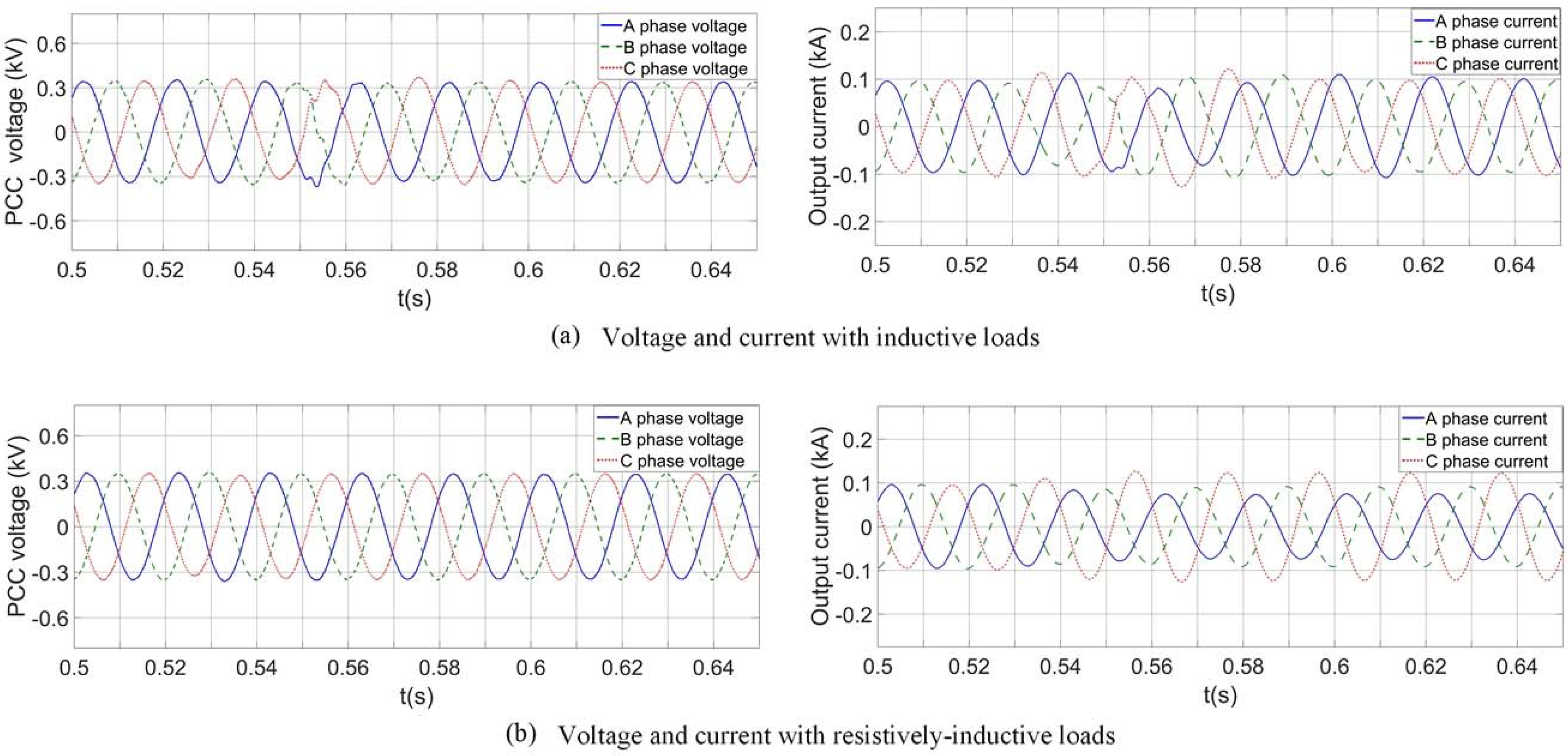
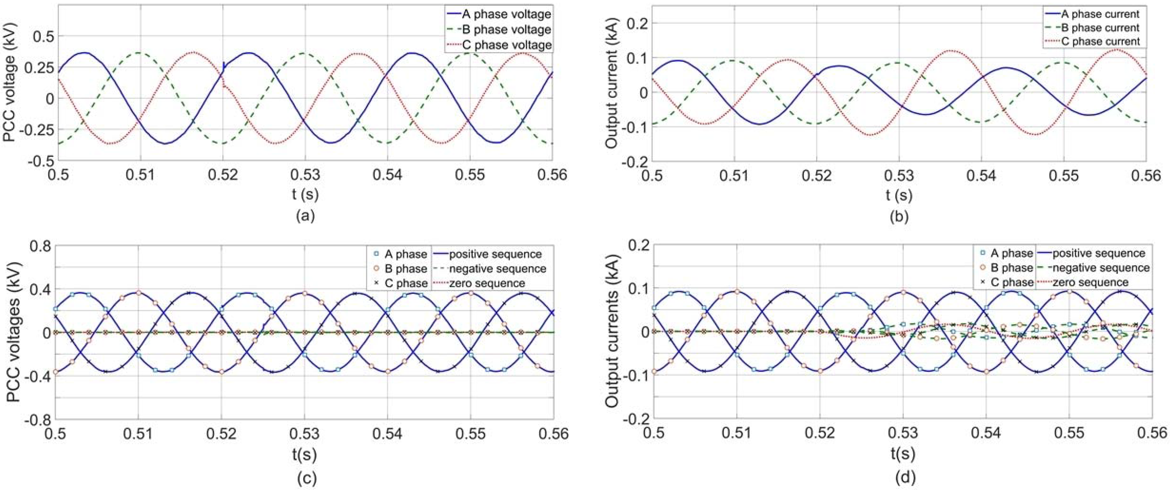
4.1. Verification of the Voltage-Balancing Capability of the Control Strategy

Voltage unbalance of the distribution network is mainly caused by load asymmetry, so the impedance change of the load is applied to verify the voltage-balancing capability of the control strategy.

Firstly, a tunable three-phase resistor $R$ is used as the load in simulation. At the very beginning of the simulation, $R_{\mathrm{a}}$, $R_{\mathrm{b}}$, and $R_{\mathrm{c}}$ are all set as 10 Ω. At 0.52 s in simulation, $R_{\mathrm{a}}$ increases to 20 Ω and $R_{\mathrm{c}}$ decreases to 5 Ω. The voltage and current waveforms can be obtained through simulation.

In Figure 12a, there is a minor disturbance to the three-phase voltage when the resistances of the load changes at 0.52 s, and the voltage regains symmetry quickly afterwards. By contrast, in Figure 12b, the three-phase current becomes asymmetric after the load change. In Figure 12c,d, where the voltage and current are decomposed into positive, negative, and zero sequence components, the negative and zero sequence voltages disappear right after its occurrence at 0.52 s, while the corresponding currents have been existing ever since this moment. This is an indication of the fast response of the control system.

Besides the simulation with the resistive loads, simulations with inductive loads and resistively-inductive loads are also carried out. At the very beginning of the simulation, the inductive loads $L_{\mathrm{a}}$, $L_{\mathrm{b}}$, and $L_{\mathrm{c}}$ are all set as 30 mH. At 0.52 s, $L_{\mathrm{a}}$ grows to 60 mH and $L_{\mathrm{c}}$ falls to 15 mH. The output voltage and current performances in this case are shown in Figure 13a. The three phase resistances of the resistively-inductive loads $R_{\mathrm{a}}$, $R_{\mathrm{b}}$, and $R_{\mathrm{c}}$ are all set as 10 Ω while the inductance $L_{\mathrm{a}}$, $L_{\mathrm{b}}$, and $L_{\mathrm{c}}$ are set as 10 mH. At 0.52 s in simulation, $R_{\mathrm{a}}$ grows to 20 Ω, $L_{\mathrm{a}}$ grows to 20 mH, $R_{\mathrm{c}}$ falls to 5 Ω, and $L_{\mathrm{c}}$ falls to 5 mH. The simulation results of output voltages and currents are presented in Figure 13b.

As is shown in Figure 13, when the inductive and resistively-inductive loads change, the voltages in both cases can transition to three-phase symmetrical conditions fast. The transition period with inductive loads is slightly longer than that with resistively-inductive loads, but finally both of the voltages can get symmetrical within 0.06 s.

From the simulation results, it is concluded that the three-phase four-leg inverter with this control strategy can ensure the output voltage balance.

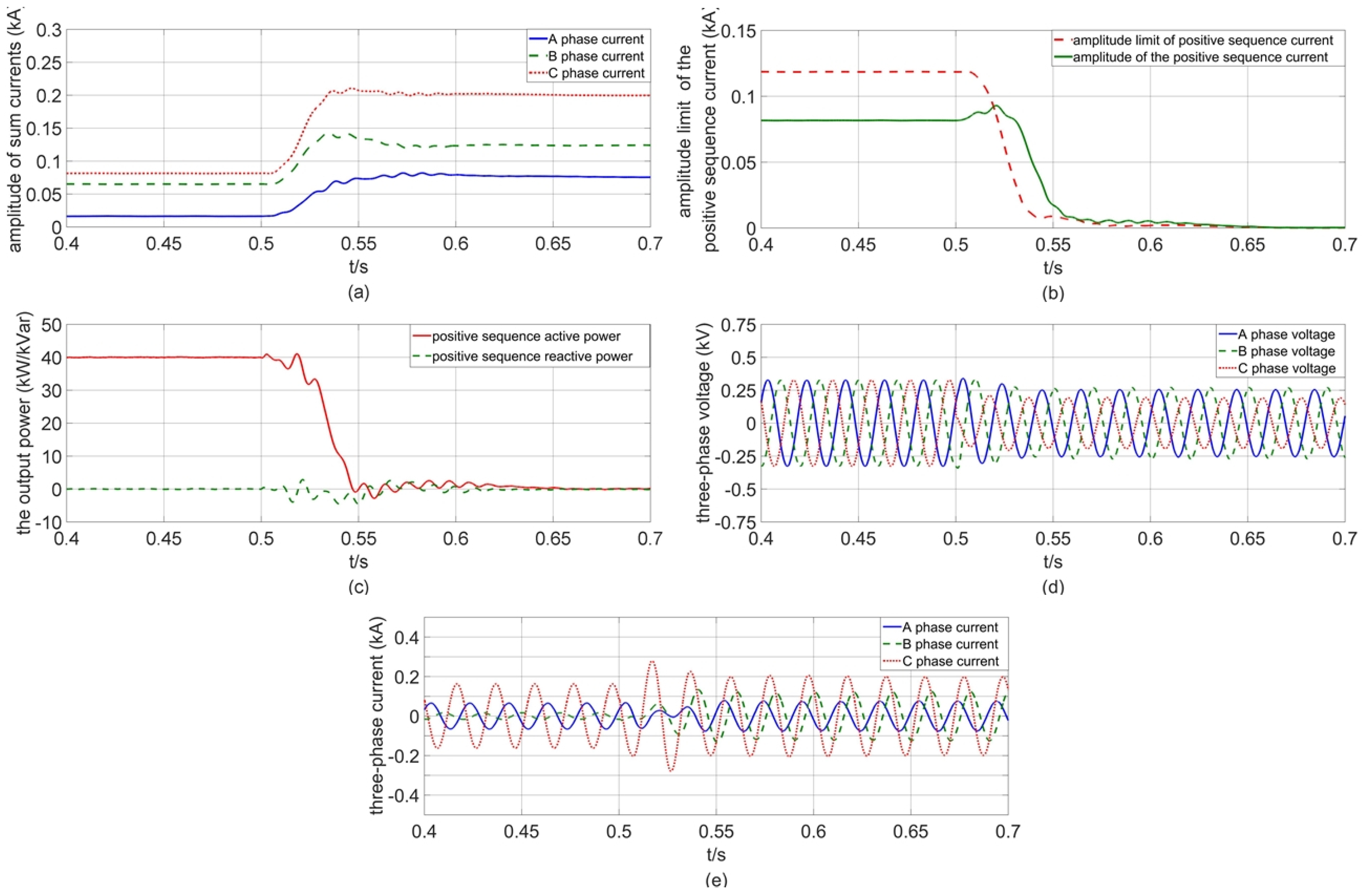
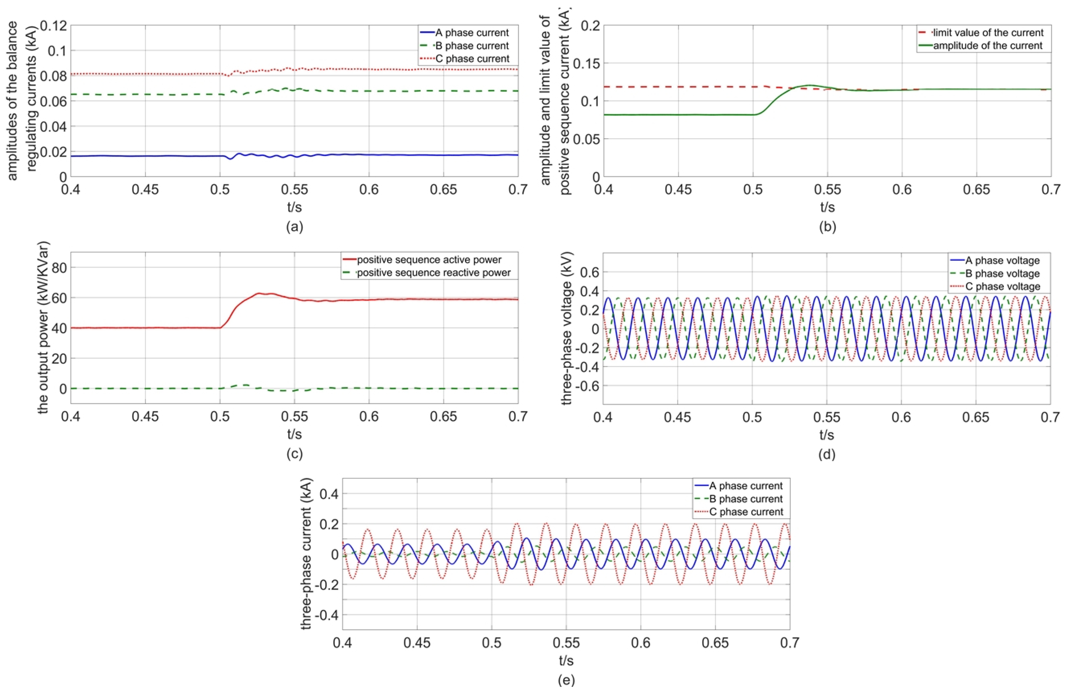
4.2. Verification of the Current-Limiting Scheme

The current-limiting capability of the scheme has been tested in two cases—where a large reference power is given and where a severely unbalanced load is applied. For the model in Figure 11, it is assumed that $R_{\mathrm{a}}$ is set as 10 Ω, $R_{\mathrm{b}}$ is set as 5 Ω, and $R_{\mathrm{c}}$ is set as 2 Ω. So the load is unbalanced. The active power reference is set as 40 kW and the reactive power is 0. The amplitude limit of the phase current is set as 0.2 kA. The current-limiting scheme is designed with the priority of voltage balance.

Case (1): The case is used to test the current-limiting capability while the current increase is caused by the ascent of the output reference of inverter. In this case, the active power reference is changed to 70 kW at 0.5 s, the external load condition keeps constant. The simulation results are shown in Figure 14.

In Figure 14a, the amplitude of the sum of negative and zero sequence currents for each phase is presented. When the active power reference changes to 70 kW, each of them increases slightly, but they are still under the limit of 0.2 kA. Therefore, the PCC voltage in Figure 14d is still three-phase symmetrical. Accordingly, in Figure 14b, the limit value of the positive sequence current has a slight drop. To output more power, the positive sequence current rises before it is capped at the limit value. Therefore, in Figure 14c, the active power output by the inverter fails to reach the reference, but finally stops at around 58 kW. In a word, the output power is limited to ensure the current of each phase will not go beyond the set limit. According to Figure 14e, the current of phase C is the largest whose amplitude is limited at 0.2 kA.

In case (1), the three phase currents are all no more than the limit and the three phase voltages are symmetrical throughout. The increase of the output power reference only has a minor influence on the negative and zero sequence currents through the slight variation of the voltage. Therefore, the voltage-balancing capability can be ensured by the embedded current-limiting scheme with different output reference.

Case (2): The case is used to test the current-limiting capability while the current increase is caused by the deterioration of the external load asymmetry. At 0.5 s, the resistance of phase C changes from 2 to 0.5 Ω. The unbalanced load is introduced to show the adjusting process and performance of the currents while the voltage unbalance rises beyond the capacity of control strategy under the constraint of the current-limiting scheme. The simulation results are shown as Figure 15.

In Figure 15a, the amplitude of the sum of the negative and zero sequence currents in phase C has reached the limit. The inverter is supposed to maintain voltage symmetry to its greatest capacity yet fails to achieve the goal due to the severe asymmetry of the load. So in Figure 15d, the PCC voltage cannot keep balanced after 0.5 s. Also, in Figure 15b, the limit value of the positive sequence current drops to 0, which causes the positive sequence active power to fall to 0 in Figure 15c. According to Figure 15d, it can be seen that the largest phase current appears in phase C, and it has an impulse to exceed the amplitude limit of 0.2 kA, but finally stabilizes under the limit.

In case (2), with the asymmetry increasing, the inverter needs to output larger negative and zero sequence currents to maintain voltage symmetry, which may cause the currents to exceed the limit. As the priority of the current-limiting scheme is voltage balance, the negative and zero sequence currents are preferentially output. So the positive sequence current drops to 0 to give way to the negative and zero sequence currents in this case. The voltage finally becomes asymmetrical because the demand of the negative and zero sequence currents to maintain the voltage symmetry is beyond the limit of the current-limiting scheme.

5. Conclusions

In the paper, a novel control strategy including an adaptive current-limiting scheme for grid-connected three-phase four-leg inverter is proposed. It has the capability to dynamically adjust the current limit of each sequence while keeping the output voltage symmetrical. The main features are listed as follows:

• The independent control schemes for the positive, negative, and zero sequence in synchronous rotating frame are realized based on the symmetrical component method. All three sequence components are transformed into DC to make the PI controller applicative.
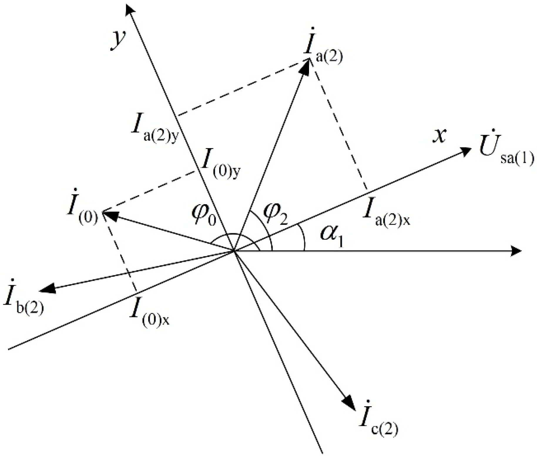
• Through the coordinate transformation, all the DC components of the three sequence currents in d-q frames are unified into one coordinate system. The current limiter is designed by calculating the current reference of each sequence in this unified coordinate system.
• The current-limiting scheme is adaptive to the output power reference and the loads asymmetry condition. It can set the current limit of each sequence reasonably while giving full play to the output capability of the inverter.

References

1. Miveh, M.R.; Rahmat, M.F.; Ghadimi, A.A.; Mustafa, M.W. Control techniques for three-phase four-leg voltage source inverters in autonomous microgrids: A review. Renew. Sustain. Energy Rev. 2016, 54, 1592–1610. [Google Scholar] [CrossRef]
2. Li, Y.W.; Vilathgamuwa, D.M.; Loh, P.C. Microgrid power quality enhancement using a three-phase four-wire grid-interfacing compensator. IEEE Trans. Ind. Appl. 2005, 41, 1707–1719. [Google Scholar] [CrossRef]
3. Olivares, D.E.; Mehrizi-Sani, A.; Etemadi, A.H.; Canizares, C.A.; Iravani, R.; Kazerani, M.; Hajimiragha, A.H.; Gomis-Bellmunt, O.; Saeedifard, M.; Palma-Behnke, R.; et al. Trends in microgrid control. IEEE Trans. Smart Grid 2014, 5, 1905–1919. [Google Scholar] [CrossRef]
4. Rivera, M.; Yaramasu, V.; Llor, A.; Rodriguez, J.; Wu, B.; Fadel, M. Digital predictive current control of a three-phase four-leg inverter. IEEE Trans. Ind. Electron. 2013, 60, 4903–4912. [Google Scholar] [CrossRef]
5. Sun, C.; Ma, W.M.; Lu, J.Y. Analysis of the unsymmetrical output voltages distortion mechanism of three-phase inverter and its corrections. Proc. CSEE 2006, 26, 57–64. [Google Scholar]
6. Dou, X.B.; Quan, X.J.; Hu, Q.R.; Wu, Z.J.; Zhao, B.; Li, P.; Zhang, S.Z.; Jiao, Y. An optimal PR control strategy with load current observer for a three-phase voltage source inverter. Energies 2015, 8, 7542–7562. [Google Scholar] [CrossRef]
7. Lai, N.B.; Kim, K.H. An improved current control strategy for a grid-connected inverter under distorted grid conditions. Energies 2016, 9, 190. [Google Scholar] [CrossRef]
8. Savaghebi, M.; Jalilian, A.; Vasquez, J.C.; Guerrero, J.M. Autonomous voltage unbalance compensation in an islanded droop-controlled microgrid. IEEE Trans. Ind. Electron. 2013, 60, 1390–1402. [Google Scholar] [CrossRef]
9. Guo, X.H.; Chang, C.W.; Chang-Chien, L.R. An automatic voltage compensation technique for three-phase stand-alone inverter to serve unbalanced or nonlinear load. In Proceedings of the 2015 IEEE international future energy electronics conference (IFEEC), Taipei, Taiwan, 1–4 November 2015.
10. Bozalakov, D.V.; Vandoorn, T.L.; Meersman, B.; Papagiannis, G.K.; Chrysochos, A.I.; Vandevelde, L. Damping-based droop control strategy allowing an increased penetration of renewable energy resources in low-voltage grids. IEEE Trans. Power Deliv. 2016, 31, 1447–1455. [Google Scholar] [CrossRef]
11. Stala, R. A natural DC-link voltage balancing of diode-clamped inverters in parallel systems. IEEE Trans. Ind. Electron. 2013, 60, 5008–5018. [Google Scholar] [CrossRef]
12. Tian, K.; Wu, B.; Narimani, M.; Xu, D.; Cheng, Z.Y.; Zargari, N.R. A capacitor voltage-balancing method for nested neutral point clamped (NNPC) inverter. IEEE Trans. Power Electron. 2016, 31, 2575–2583. [Google Scholar] [CrossRef]
13. Liu, Z.; Liu, J.J.; Li, J. Modeling, analysis, and mitigation of load neutral point voltage for three-phase four-leg inverter. IEEE Trans. Ind. Electron. 2013, 60, 2010–2021. [Google Scholar] [CrossRef]
14. Gu, H.R.; Wang, D.Y.; Shen, H.; Zhao, W.; Guo, X.Q. Research on control scheme of three-phase four-leg inverter. Power Syst. Prot. Control 2011, 39, 41–46. [Google Scholar]
15. Bayhan, S.; Trabelsi, M.; Abu-Rub, H. Model predictive control of Z-source four-leg inverter for standalone photovoltaic system with unbalanced load. In Proceedings of the 2016 IEEE applied power electronics conference and exposition (APEC), Long Beach, CA, USA, 20–24 March 2016.
16. Guo, Z.Q.; Panda, S.K.; Prasanna, I.V. Design of new control strategies for a four-leg three-phase inverter to eliminate the neutral current under unbalanced loads. In Proceedings of 2014 international power electronics conference (IPEC-Hiroshima 2014-ECCE ASIA), Hiroshima, Japan, 18–21 May 2014.
17. Su, M.; Wang, H.; Sun, Y.; Tan, J.M.; Yu, J.R.; Gui, W.H. Design of three-phase four-leg inverter based on modified repetitive controller. Proc. CSEE 2010, 30, 29–35. [Google Scholar]
18. Chen, H.B.; Min, J.Y. Simulation research on the control strategy of three-phase four-leg inverter. In Proceedings of the 2010 international conference on computer application and system modeling (ICCASM 2010), Taiyuan, China, 22–24 October 2010.
19. Vechiu, I.; Curea, O.; Camblong, H. Transient operation of a four-leg inverter for autonomous applications with unbalanced load. IEEE Trans. Power Electron. 2010, 25, 399–407. [Google Scholar] [CrossRef]
20. Golwala, H.; Chudamani, R. New Three-dimensional space vector-based switching signal generation technique without null vectors and with reduced switching losses for a grid-connected four-leg inverter. IEEE Trans. Power Electron. 2016, 31, 1026–1035. [Google Scholar] [CrossRef]
21. Ozdemir, A.; Erdem, Z. Optimal digital control of a three-phase four-leg voltage source inverter. Turk. J. Electr. Eng. Co. 2016, 24, 2220–2238. [Google Scholar] [CrossRef]
22. Zhang, R.; Prasad, V.H.; Boroyevich, D. Three-dimensional space vector modulation for four-leg voltage-source converters. IEEE Trans. Power Electron. 2002, 17, 314–326. [Google Scholar] [CrossRef]
23. Akagi, H.; Watanabe, E.H.; Aredes, M. Instantaneous Power Theory and Applications to Power Conditioning, 1st ed.; Xu, Z., Ed.; China machine press: Beijing, China, 2009; pp. 60–63. (In Chinese) [Google Scholar]
24. Zhang, X.; Zhang, C.W. PWM Rectifier and its Control, 1st ed.; China machine press: Beijing, China, 2012; pp. 14–117. [Google Scholar]
25. Wang, C.S.; Li, Y.; Peng, K. Overview of Typical Control Methods for Grid-Connected Inverters of Distributed Generation. Proc. CSU-EPSA 2012, 24, 12–20. [Google Scholar]
26. Zhang, N.Y.; Tang, H.J.; Yao, C. A systematic method for designing a PR controller and active damping of the LCL filter for single-phase grid-connected PV inverters. Energies 2014, 7, 3934–3954. [Google Scholar] [CrossRef]
27. Shi, C.W. Research on the Control Method of Three-Phase Inverter under Unbalanced Loads. Master’s Thesis, Southwest Jiaotong University, Chengdu, China, 1 May 2014. [Google Scholar]
Figure 1. Topological structure of three-phase four-leg inverter with LC filter.
Energies 09 00726 g001
Figure 2. Equivalent circuit topology of zero sequence.
Energies 09 00726 g002
Figure 3. Control strategy of the three-phase four-leg inverter: (a) Positive sequence control strategy; (b) Negative sequence control strategy.
Energies 09 00726 g003
Figure 4. The transformation process of zero sequence.
Energies 09 00726 g004
Figure 5. Superimposition of control signals.
Energies 09 00726 g005
Figure 6. Positive sequence current in d-q frame.
Energies 09 00726 g006
Figure 7. The positive sequence modulus limiter.
Energies 09 00726 g007
Figure 8. Phasor diagram of the negative sequence and zero sequence currents in x-y frame.
Energies 09 00726 g008
Figure 9. The negative and zero sequence modulus limiter.
Energies 09 00726 g009
Figure 10. Method to get the maximum of the positive sequence current.
Energies 09 00726 g010
Figure 11. Distribution network with a three-phase four-leg inverter-based DG.
Energies 09 00726 g011
Figure 12. Waveforms of the PCC voltage and output current: (a) Three-phase voltage; (b) Three-phase current; (c) The positive, negative, and zero sequence voltages; (d) The positive, negative, and zero sequence currents.
Energies 09 00726 g012
Figure 13. Waveforms of voltages and currents with inductive and resistively-inductive loads: (a) The inductive loads change; (b) The resistively-inductive loads change.
Energies 09 00726 g013
Figure 14. Simulation results of the case with the power reference changing: (a) The amplitudes of the balance regulating currents; (b) The positive sequence current and its amplitude limit; (c) The active power and reactive power outputted by the inverter; (d) The three-phase PCC voltage; (e) The three-phase output current.
Energies 09 00726 g014
Figure 15. Simulation results in the case with load changing: (a) The amplitudes of the balance regulating currents; (b) The positive sequence current and its amplitude limit; (c) The active power and reactive power output by the inverter; (d) The three-phase PCC voltage; (e) The three-phase output current.
Energies 09 00726 g015