Numerical Simulation of the Depressurization Process of a Natural Gas Hydrate Reservoir: An Attempt at Optimization of Field Operational Factors with Multiple Wells in a Real 3D Geological Model

Sun, Zhixue; Xin, Ying; Sun, Qiang; Ma, Ruolong; Zhang, Jianguang; Lv, Shuhuan; Cai, Mingyu; Wang, Haoxuan

doi:10.3390/en9090714

Open AccessArticle

Numerical Simulation of the Depressurization Process of a Natural Gas Hydrate Reservoir: An Attempt at Optimization of Field Operational Factors with Multiple Wells in a Real 3D Geological Model

¹

School of Petroleum Engineering, China University of Petroleum (East China), Qingdao 266580, China

²

College of Energy Resources, Chengdu University of Technology, Chengdu 610059, China

^*

Authors to whom correspondence should be addressed.

Energies 2016, 9(9), 714; https://doi.org/10.3390/en9090714

Submission received: 6 May 2016 / Revised: 17 August 2016 / Accepted: 22 August 2016 / Published: 6 September 2016

Download

Browse Figures

Versions Notes

Abstract

:

Natural gas hydrates, crystalline solids whose gas molecules are so compressed that they are denser than a typical fluid hydrocarbon, have extensive applications in the areas of climate change and the energy crisis. The hydrate deposit located in the Shenhu Area on the continental slope of the South China Sea is regarded as the most promising target for gas hydrate exploration in China. Samples taken at drilling site SH2 have indicated a high abundance of methane hydrate reserves in clay sediments. In the last few decades, with its relatively low energy cost, the depressurization gas recovery method has been generally regarded as technically feasible and the most promising one. For the purpose of a better acquaintance with the feasible field operational factors and processes which control the production behavior of a real 3D geological CH₄-hydrate deposit, it is urgent to figure out the effects of the parameters such as well type, well spacing, bottom hole pressure, and perforation intervals on methane recovery. One years’ numerical simulation results show that under the condition of 3000 kPa constant bottom hole pressure, 1000 m well spacing, perforation in higher intervals and with one horizontal well, the daily peak gas rate can reach 4325.02 m³ and the cumulative gas volume is 1.291 × 10⁶ m³. What’s more, some new knowledge and its explanation of the curve tendency and evolution for the production process are provided. Technically, one factor at a time design (OFAT) and an orthogonal design were used in the simulation to investigate which factors dominate the productivity ability and which is the most sensitive one. The results indicated that the order of effects of the factors on gas yield was perforation interval > bottom hole pressure > well spacing.

Keywords:

gas hydrate; geological model; simulation; depressurization method; Shenhu Area

Graphical Abstract

1. Introduction

1.1. Background

The global temperature of the Earth’s atmosphere is rising due to human emissions of greenhouse gases, especially carbon dioxide produced by fossil fuel combustion [1]. Since the beginning of the Western Industrial Revolution, the acquisition of clean, secure and sustainable energy sources has been the future and foundation of the world’s increasing economic growth [2]. As a substitute for fossil fuel and potential source of energy, natural gas hydrates are drawing global scientists’ attention and playing an important part in resolving the energy crisis and climate change issues [3]. Figure 1 indicates that they are wildly distributed around the global, being found in particularly large quantities as sediments deposited on the deep ocean floor and as permafrost on the continental plateaus [4]. Natural gas hydrates are crystalline solids composed of small gas molecules and water in which the gas molecules are extremely compressed, making them denser than typical fluid hydrocarbons [5]. The rough estimated volume of gas that could be released from the hydrate reservoirs all over the world already exceeds that of known traditional gas resources [6]. It is probable that we will use the new environmentally friendly fuel source to meet the increasing demand for energy in the next two decades. In terms of various areas worldwide, Figure 1 compares the reserve volume of methane hydrate. Consequently, we can draw the conclusion gas hydrates are one kind of new energy with great promise in the future [1].

The following equation describes the essence of hydrate formation and dissociation and the direction of the reaction:

{CH}_{4} {+ N}_{H} H_{2} O \Leftrightarrow {CH}_{4} \cdot N_{H} H_{2} O + Δ H

(1)

where N_H is the hydration number and N_H = 5.75 is the complete hydration number, while N_H = 6.0 corresponds to the average number. ΔH is the enthalpy of the formation and dissociation reactions [6]. The hydration process in Equation (1) has also been thoroughly studied in the past few years as a promising method to separate methane from gaseous mixtures [8,9,10,11]. Recently, several ways of developing hydrate reservoirs (Figure 2) have been put forward, including thermal stimulation [12,13,14], injection of hot brine, steam or hot water to heat the hydrate reservoir to exceed the dissociation temperature; depressurization [15,16,17], to lower the original pressure of hydrate reservoir under the dissociation pressure at a specific temperature; thermodynamic inhibitor injection [18,19], to change the hydrate pressure-temperature equilibrium conditions by injecting chemicals, such as alcohols and salts; and CO₂ exchange which is most promising method to reduce the emissions of greenhouse gases [20,21]. Figure 3 indicates the former three methods presented above are based on the mechanism that changes the pressure or temperature condition to destroy the stability of the original equilibrium of the hydrate deposit, resulting in its dissociation and the production of methane. However, with the relatively low energy cost and economic effectiveness, the depressurization method is generally regarded as technically feasible and the most promising one for field hydrate dissociation in the last few decades [22,23,24]. In accordance with the research results published in [25], the Mallik 2002 well proved that it is feasible to use a combination of thermal stimulation and depressurization to obtain gas from permafrost [26]. Recent studies have also demonstrated that using vertical wells technology to produce gas from natural hydrate reservoirs can maintain high rates for a long period in certain cases, as described by Li and Kurihara et al. [22,24]. However, there is also simulation research indicating that using horizontal wells has tremendous advantages over vertical wells to obtain the gas from Class 2 and Class 3 hydrate deposits (e.g., Moridis [27] and Wang et al. [28]). However, a single well was used in all of these numerical depressurization stimulations with theoretical models. No research results about numerical depressurization stimulation with a multiple well in an actual geological CH₄-hydrate deposit model have been reported yet. In practice, there is a tendency and need to use multi-well systems to develop a hydrate reservoir field. Therefore, it is quite interesting to simulate the dissociation process and the production behaviors in a real 3D geological CH₄-hydrate deposit model with a multi-well system [28].

1.2. Status Quo in Hydrate Reservoir Modeling

Due to the complexity of the underground environment, numerical models and simulations have a great significance in the study of gas hydrate reservoir development. In recent years, various numerical simulation programs such as MH-21 HYDRES, Transport of Unsaturated Groundwater and Heat (TOUGH) + HYDRATE, HydrateResSim, STOMP-HYD and the Computer Modelling Group-Advanced Processes & Thermal Reservoir Simulator (CMG STARS) have been developed [29].

CMG–STARS which is a commercial black oil reservoir simulator can describe hydrate reservoirs. This simulator includes the Kim–Bishnoi kinetic parameters that can describe heat of dissociation and hydrate thermodynamic stability which is the core mechanism for hydrate simulation [30]. Compared with other software that can be adapted to describe hydrate reservoirs, its accuracy and suitability to represent production performance from hydrate deposit in porous media has been validated by many researchers (e.g., [29,31,32]). TOUGH + HYDRATE, originated and developed at the Lawrence Berkeley National Laboratory was the first available model to simulate hydrate reservoirs, it can take in four mass components (i.e., inhibitors, water, hydrate, and methane) partitioned between four possible phases (ice, water, gas and hydrate,) and fully couple reservoir heat transfer and mass to simulate the non-isothermal dissociation process, as described by Moridis [33]. The STOMP-HYD simulator uses the integral volume differencing with orthogonal grids for spatial discretization to solve the dominating conservation equations (White et al. [34]). HydrateResSim, an open-source code through the National Energy Technology Laboratories, is modified for binary and ternary hydrates, as mentioned by Garapati [35]. MH-21 HYDRES was developed by the Production Method and Modeling Group to estimate production process for methane hydrate simulation, what’s more, their core-test studies indicated that lowing the reservoir pressure may be the most feasible method for hydrate reservoirs at the Eastern Nankai Trough (Masuda et al. [36]). Considering the strengths and adaptability of each numerical simulation program, in this study CMG STAR was chosen as the tool to simulate the hydrate development process [37].

1.3. Objectives

The main objective of this study was to gain a better understanding of the feasible field operational factors and production processes which control the production behavior of a real 3D geological CH₄-hydrate deposit in the Shenhu Area of the South China Sea, and to carry out a systematic sensitivity analysis of the effects of the operational parameters such as well type, well spacing, bottom hole pressure, and perforated intervals on methane recovery. Several possible production methods and combination of different operational parameters are simulated and assessed.

2. Geological Model and Simulation Scenarios

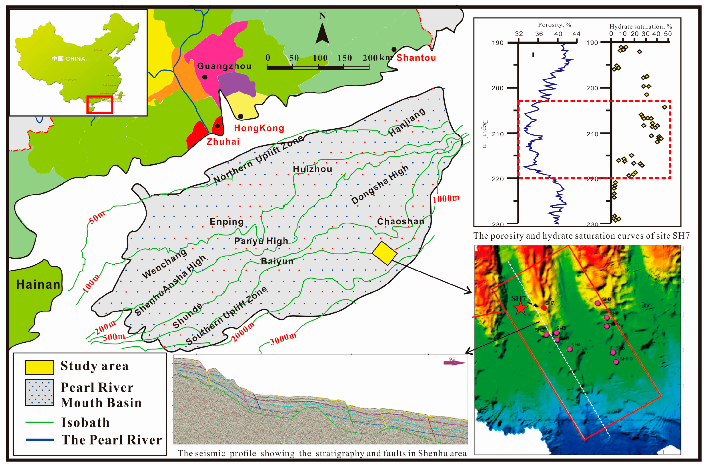
2.1. Geological Settings and Real Model

As shown in Figure 4, the Shenhu Area is located in the near southeast edge of the Shenhu Underwater Sandy Bench in the middle of the north slope of the South China Sea, between the Xisha Trough and the Dongsha Islands [38]. Tectonically, the research area is located in the Zhu II Depression of the Pearl River Mouth Basin, which has been in a process of tectonic subsidence since the middle Miocene. In China, thegas hydrate samples were first collected at three sites (SH2, SH3, and SH7) during a recent scientific expedition conducted by the China Geological Survey in the Shenhu area of the northern South China Sea in May 2007 [39,40]. Subsequently, the second Chinese marine hydrate expedition GMGS2 was performed in the Dongsha Area of the South China Sea in the summer of 2013. The hydrate resources appear to be abundant in Pearl River Mouth Basin, which has attracted much attention as a potentially important area for gas hydrate research and development in China.

According to the basic principle of governing equations (see Appendix A), based on currently available data from site measurements of eight wells, including water depth, thickness of the hydrate-bearing layer (HBL), the logging data, core porosity, the intrinsic permeability and seismic exploration interpretation data of the reservoir, a stochastic modeling method was employed to establish the real geological model of the target area. The top of the hydrate-bearing layers is buried 155–229 m below the seafloor (MBSF), and their thickness varies from 10 to 43 m. These hydrate layers are located at a water depth of 1108–1245 m. Porosity and permeability, which represent the physical properties of hydrate-bearing formation, were obtained from the laboratory analysis of the actual core and well logging interpretation. Using a sequential Gaussian simulation method, a porosity and permeability 3D distribution model of the hydrate-bearing layers was established. The layer porosity and hydrate saturation in the study area varies between 25%–46% and 20%–43%, respectively. As shown in Figure 5, the porosity and permeability distributions are the most important properties of the actual geological model which can reflect the core difference between the actual and ideal model about the influence of operational conditions.

2.2. Reservoir Parameters and Component Setting

This section builds a real 3D geological model on the basis of the actual geological data from the Shenhu case. Its size was 94 grids in the I-direction and 118 grids in the J-direction with a 50 m × 50 m grid, and the total area is 27.73 km². In the K-direction, the model is divided unequally into 40 layers from the depth of 195 m to 229 m. Consequently, there are in total 433,680 elements. The surrounding boundaries of the model were assumed to be closed.

In the simulation process of gas hydrate development, several field operational factors are considered as being relevant and necessary for the production from an actual geological CH₄-hydrate deposit. The most important actual field operational factors which will be discussed in the subsequent sections are: well spacing (WS), bottom hole pressure (BHP), well type (WT) and perforation intervals (PI).

Table 1 summarizes the main simulation model parameters which were used in the model. Values for the actual field operational factors in the table were selected to create a reference case and subsequently discuss and analyze the spatial distribution of some parameters in the third section. Then we will use a sensitivity analysis of the actual field operational factors to discuss and put forward some personal observations about methane recovery in the fourth section.

2.3. Scenarios & Simulation

This section illustrates several scenarios about how the sensitivity analysis are made. As to the four primary actual field operational factors (well spacing, BHP, well type and perforation intervals), we establish a base case (Table 1) and then vary some factors to some degree while the other factors remain fixed at the initial (base case) value (Table 2).

3. Production Performance from Some Sites in the Shenhu Area

3.1. Reference Case and Gas Production

The main simulation model parameters pertaining to the reference case are listed in Table 1. The combination of the field condition of reference case is 1000 m well spacing, BHP is 3000 kPa, vertical well and perforated in 4–13 layers. Figure 6 shows the evolution of the daily rate of gas production and the cumulative gas production. The 1 year production process can be divided into three periods, and the dashed lines express the borders of the different periods. Note that the daily gas production rises up rapidly to point A at around the 10th day and the rate is 753.37 ST m³/day, then the speed of the rise slows down and remains steady. The local maximum of gas rate daily is 4182.46 ST m³/day before a decline begins at about point B, on the 230th day, and after that dividing point the daily gas rate tends to decline steadily. In the end, the cumulative volumetric gas production reaches about 1.091 × 10⁶ ST m³. This tendency is attributed to a combination of: (a) a drop in the initial pressure system of the hydrate reservoir during the whole production process because of the pressure difference between the wellbore and the hydrate, and the pressure difference is the main driving force to be considered; (b) with the solid hydrate deposit decomposing and the constant driving force of depressurization, the effective permeability in the adjacent area of the well is increasing; (c) the water from the adjacent area breakthrough to the well to alleviate the effect of depressurization on gas productivity; (d) a drop in the initial temperature system resulting from the dissociation reaction would further slow the dissociation speed, especially after 230 days’ production [12].

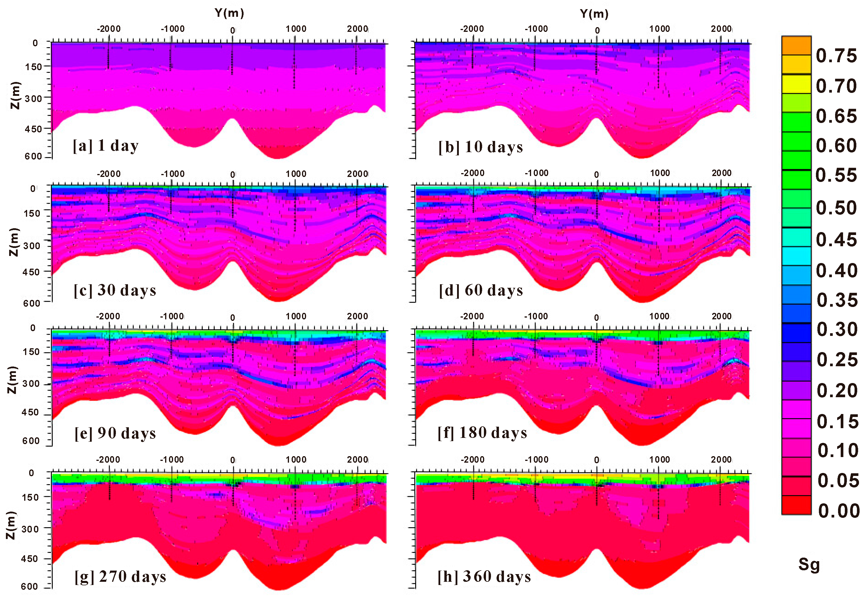
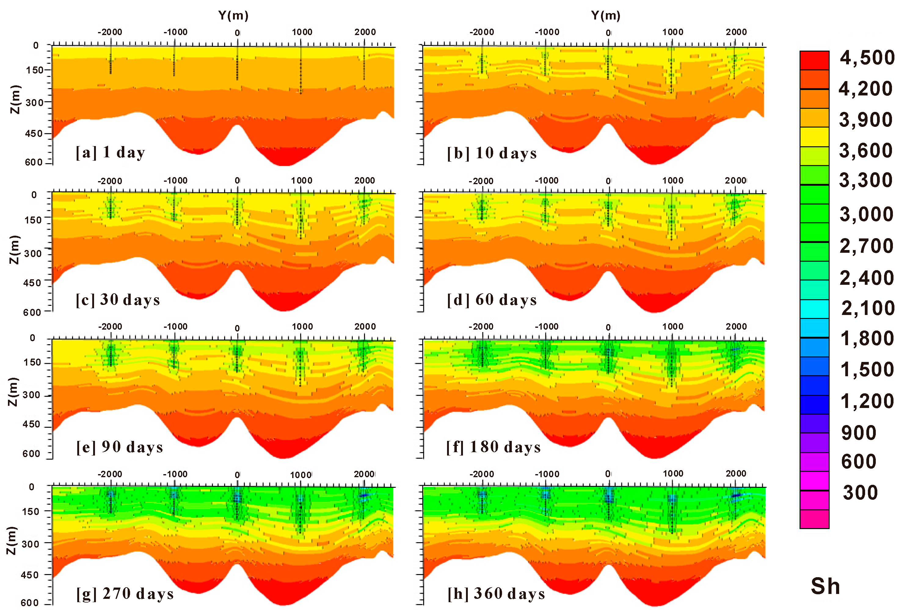
3.2. Spatial Distribution of S_g and S_h

Figure 7 and Figure 8 demonstrate the distribution evolution of the S_g and S_h in the Hydrate-Bearing Layer (HBL) during the gas production process, respectively. Figure 7 shows: (i) the waveform change of the S_g distributions; (ii) the initial hydrate dissociates at around the well and expands forward to further areas; (iii) the evolution of the dissociation interface at the upper and middle region; (iv) the accumulation of gas in the upper region. Of those, (i) are results of the characteristic porosity and permeability and the heat and fluid flow; (ii) are caused by the reasonable driving force of the continuing pressure drop and spreading pressure wave; (iii) are caused by the fluids generated from the hydrate decomposition on the lower reaction front that move toward the well in the upper area; (iv) occurs because the low effective permeability k_eff of the HBL in the upper area around the well [12].

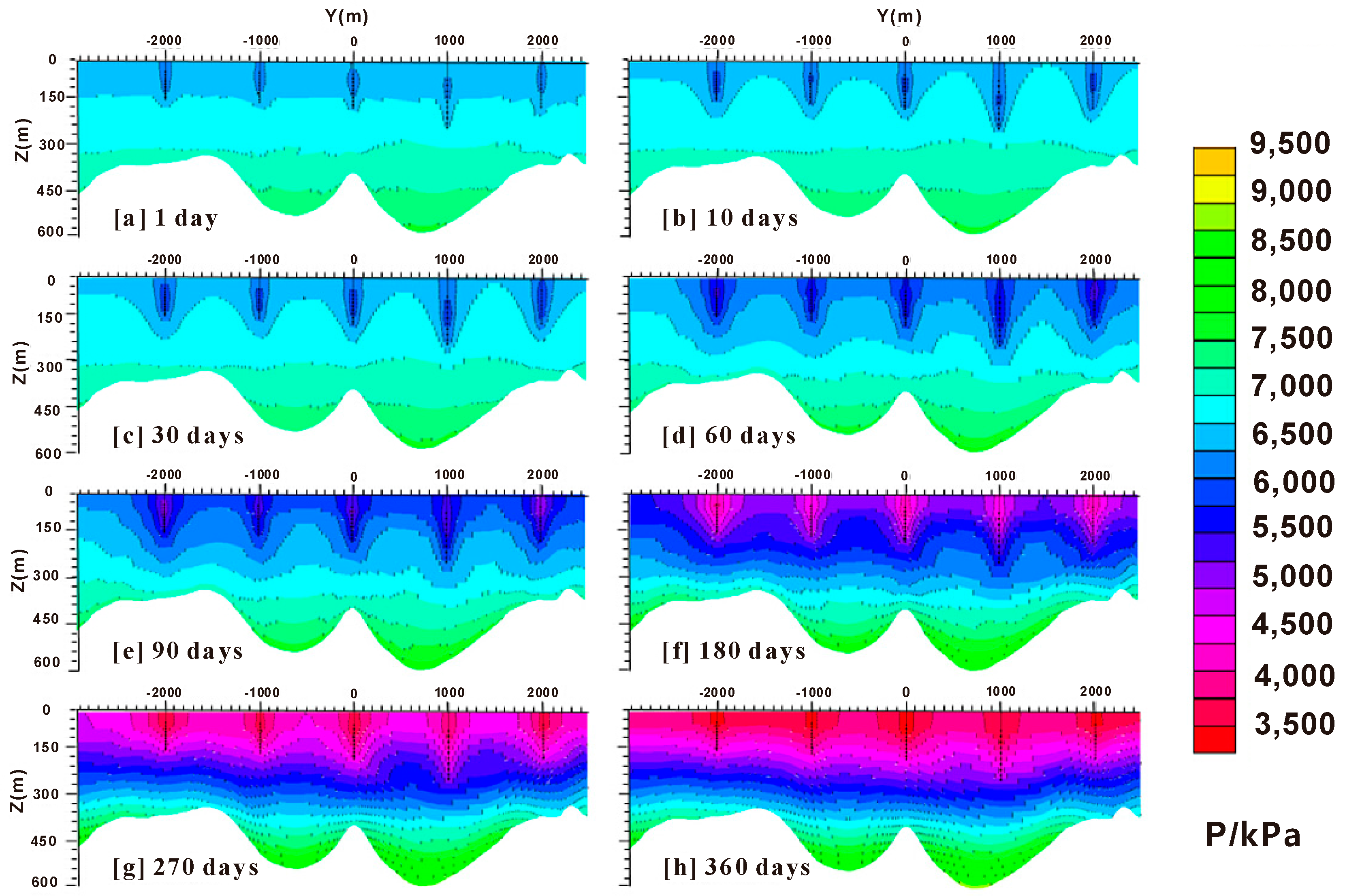
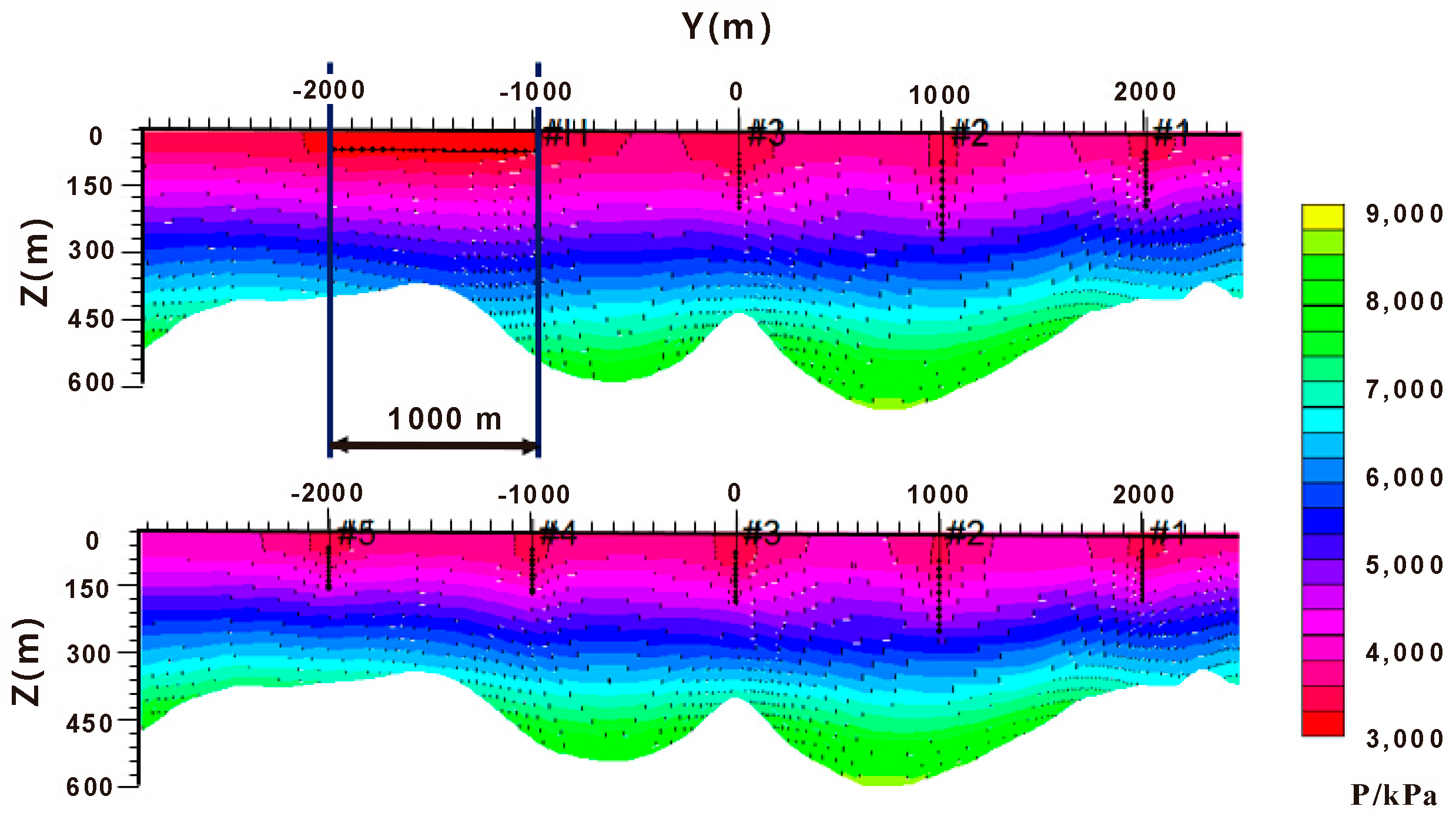
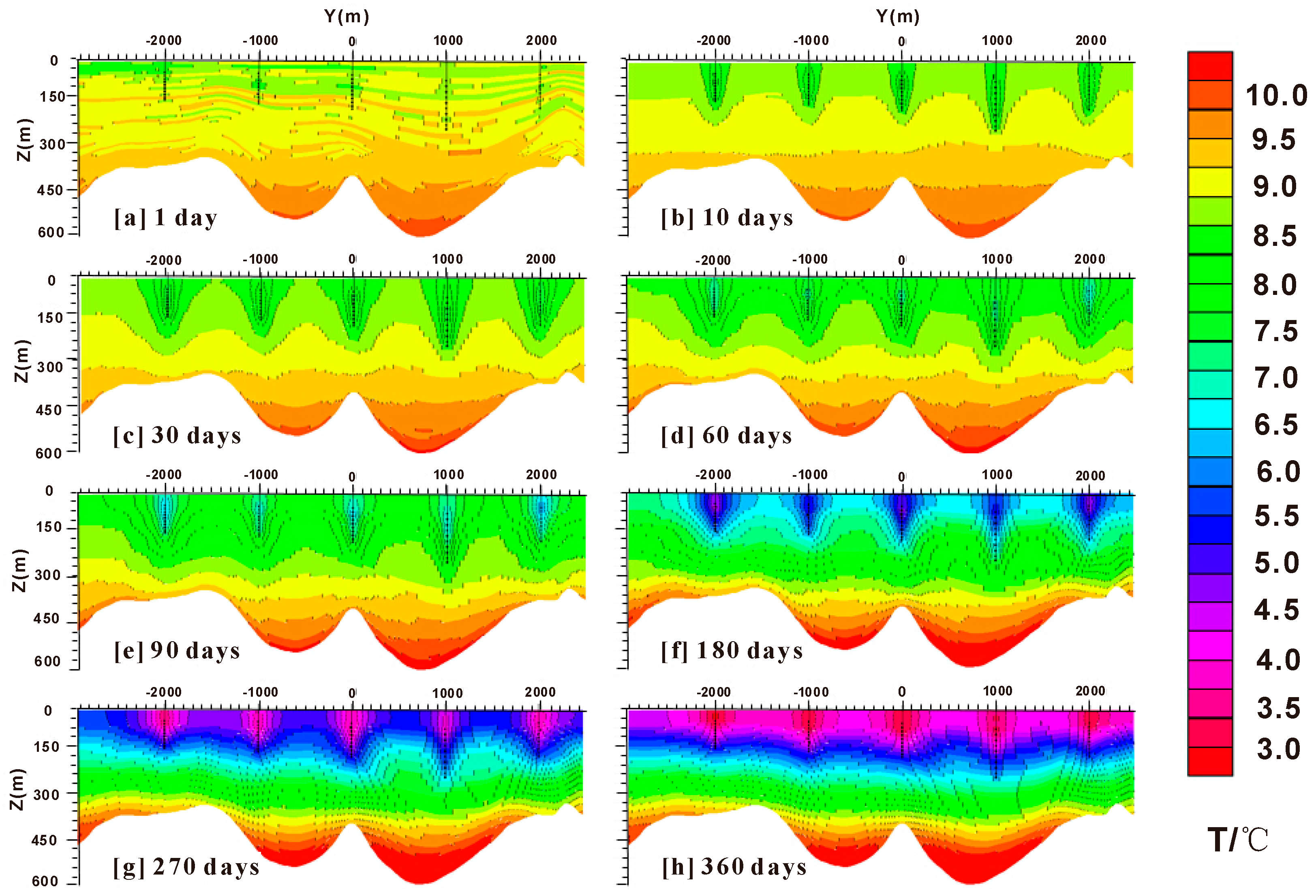
3.3. Spatial Distribution of T and P

Figure 9 and Figure 10 demonstrate the distribution evolution of the T and P during the gas production process, respectively. Figure 9 and Figure 10 show that: (i) once the initial temperature and pressure system is broken, the T and P around the well change more drastic and earlier than other areas; (ii) the drop of temperature and pressure in the lower region; (iii) the phenomenon of the jagged T distribution, P distribution is apparent and expanding and then turns to becomes weak with the development; (iv) the inflections come out at the interface of the dissociated and undissociated zone in the HBL. Of those, (i) and (ii) result from the velocity of pressure spreading and the characteristic of the thermal conductivity and permeability; and (iii) and (iv) result from the main advancing reaction front and the fluid flow of gas and water [12].

4. Results and Discussion

Before discussing the different scenarios results, it is necessary to emphasize that the aim of this study was to carry out a sensitivity analysis for feasible field operational factors based on the actual 3D geological model of Shenhu area. Although the value range of the parameters may not be applicable to other types of hydrate reservoir, the results and discussion have contributed to unveil what the most sensitive factors are and provide guidance for actual production. Figure 11, Figure 12, Figure 13, Figure 14, Figure 15 and Figure 16 present the daily gas rate, cumulative gas production and some important parameter contrasts obtained from the simulations of changing the variables one at a time.

4.1. Sensitivity of Producer Well Spacing

Producer spacing is an important parameter in hydrate reservoir development. As shown in Table 2, different well spacing scenarios (the well spacing ranged from 250 to 1000 m) were designed for analysis, and Figure 11 shows the cumulative gas production is extremely sensitive to the well spacing. The 1 years’ production process can be divided into three periods.

Before the pressure dropdown wave which is when the interactions of each well can reach an adjacent well, each scenario has an approximate trend and there is not much difference between them, which can be summarized as the initial period, Period A.

When the pressure dropdown waves of each well can interact each other at around the 10th day, the interaction with each well makes each scenario act differently until the 320th day, and we summarize this period as the interaction & storage period, which is also Period B. Although common sense would suggest that with a closer well spacing it will take the pressure dropdown wave less time to reach an adjacent well which means the pressure around the well drops faster and comes to the decomposition point easier and more decomposing gas will be produced, the results of the 250 m and 500 m well spacing scenarios show opposite trends. This phenomenon indicates that compared with pressure dropping speed, the controlling storage of each well which is reflected by the well spacing has a more powerful effect on the gas rate in this period. As for the 750 m and 1000 m scenarios, the effect of pressure interactions and controlling storage find a middle ground which makes the 750 m scenarios act best in Period B.

At approximately the 320th day, the 750 m well spacing gas rate curve and the 1000 m well spacing gas rate curves intersect with each other and after that point the 1000 m scenario produces more gas daily which indicates that the controlling storage is the conclusive factor in the long run. In the following decades the cumulative gas of 1000 m scenarios will exceed the 750 m scenario which can be predicted by the theory above and this is the so called storage period, Period C.

4.2. Sensitivity of BHP

Producer BHP is also an important parameter in the hydrate gas development. As shown in Table 2, different BHP scenarios (where the BHP ranges from 2500 to 4000 kPa) were designed for analysis. Figure 12 suggests that the cumulative gas production is extremely sensitive to the BHP, because a lower BHP results in a higher driving force, leading to a higher gas travel velocity in the HBL and in turn stimulating even more hydrate to decompose consequently. These four scenarios have the same well spacing of 1000 m, so the main force of the decomposition speed is the drawdown pressure between the hydrate reservoir pressure and the BHP, the larger the drawdown pressure is, the sooner the hydrate host formation can reach to its dissociation pressure point, and the more gas will be produced in the beginning period.

Similarly, the 1 years’ production time can also be divided into three periods on the basis of the daily gas production rate. The travel distance of the pressure dropdown wave is the same while the speed is quite different which is determined by the drawdown pressure between the hydrate reservoir and the BHP, so the faster the speed is, the sooner the pressure dropdown waves can reach other wells, and the sooner the interaction can happen. The initial period gas rate curves are different from those in Figure 11, and the four curves of Figure 12 are more disordered.

The B period can be called the speeding period because the differences of the curves are so obvious and all the gas rates are increasing which indicates the drawdown pressure effect in this period is the dominant factor and the 2500 kPa curve areis rising rapidly.

At approximately the 250th day, all the gas rate curves are declining and have a trend to coincide with each other when the gap between the hydrate reservoir pressure and the BHP becomes smaller and even vanishes. In the following decades, when the gap is gone, the reaction will come to a phase equilibrium again and no more extra gas will be produced. The accumulated gas of the 2500 kPa scenarios will no doubt be the most because the initial gap is the largest which can be predicted by the theory above and this is the so called declining period, Period C.

4.3. Sensitivity of Well Types

Well type is also an important parameter in hydrate gas development. As shown in Table 2, different well type scenarios were designed for the analysis, and Figure 13 shows that the distance between a horizontal well’s head and end is equal to the well spacing of vertical wells. Figure 14 indicates that the daily gas production is extremely sensitive to the well type at the beginning, because a horizontal well has a more effective contact area, resulting in more controlled storage and in turn stimulating even more hydrate to decompose and the pressure to drop more in the end. For a similar reason as discussed in the former sections, the rising stage can be divided into two periods, Period A and Period B. At approximately the 260th day, the two curves intersect with each other and after that point the five vertical wells scenario produces more daily gas which indicates that the use of horizontal wells in such reservoirs may not be attractive in the long run because all layers show an upward gas migration block which is contrary to gas production from conventional gas reservoirs.

4.4. Sensitivity of Perforation Intervals of Producing Well

The perforation intervals of producing wells have an extremely significant effect on the development of hydrate gas reservoirs. Figure 15 shows that under the conditions of producer well spacing of 1000 m, bottom hole pressure of 3000 kPa, perforation intervals of 4–13 layers, the cumulative gas production and daily gas rate are the largest, and the differences between different perforation intervals are so huge that one can easily distinguish them from each other. Such huge differences may be a combined consequence by many phenomena, such as the formation pressure, non-homogeneity, temperature, grids’ shape, the accuracy of program and so on. Figure 16 shows the pressure distribution of the last simulation day when perforated at different layers. It can be seen that the pressures around the perorated layers are so different that a lower pressure in the hydrate deposit produced more gas than other scenarios. The reason may be due to the fact that the upper layer has a lower initial pressure and it is easy and fast to decline to its decomposition pressure point with constant BHP. Therefore, perforation intervals have an extremely strong effect on the production. The production well perforation interval should be located in the upper deposit in the development of the Shenhu case.

4.5. Orthogonal Design

With the rapid development of numerical calculations and new computational techniques in the past few decades, reservoir simulation technology has become cost-effective for model industries, not only for maximizing the production ability by factor optimization but also for assessing new production designs. It is in this study that sensitivity analysis can be conducive to assess interactions between factors, key factor determination, production forecasting, and phenomenological understanding [41]. Sensitivity analysis is a tool for a model to systematically vary factors to confirm the effect of such changes [42]. In practice, it has been employed in several numerical reservoir studies [41,43,44]. There are two ways to put the sensitivity analysis into practice: (1) one factor at a time (OFAT); and (2) orthogonal design. OFAT is the most general means to carry out sensitivity analysis by electing a reference level for each parameter and then changing each parameter over its range while the other parameters remain unchanged [45]. Although this approach can unambiguously attribute any variation that observed in the result to the single changed parameter and increase the comparability of the results, it cannot take the interactions between the parameters which are due to the failure of one parameter to have the same effect on the response while another parameter is changed too [42].

In this paper, although the analysis of field operational conditions has been made by the OFAT in the last few sections, we still cannot draw a specific conclusion about which is the most sensitive parameter and the effect order among well spacing, bottom hole pressure and perforation intervals. Thus, we employ an orthogonal design to determine the relative importance of field operation variables on the cumulative gas produced from an actual geological CH₄-hydrate deposit. Figure 17 indicates the production performance prediction of the orthogonal design experiment.

Table 3 shows the basic data of the orthogonal design experiment and the analysis results. Mean A, B and C are taken the average value of cumulative gas in three groups of experiment, and range is the difference between the maximum and the minimum of the mean for a certain factor. The effect of factors can be analyzed by comparing the numerical value of a range, and the larger the range, the greater effect. The one factor at a time design and the orthogonal design indicate that the order of the effects of the factors on gas yield was perforation intervals > bottom hole pressure > well spacing, and the best combination of operation condition is A2, B1and C1 which is well spacing 750 m, BHP 2500 kPa and perforation in the 4–13 layers, whereby the cumulative gas production can be 1,309,742 m³.

5. Conclusions

The following conclusions can be taken from this study:

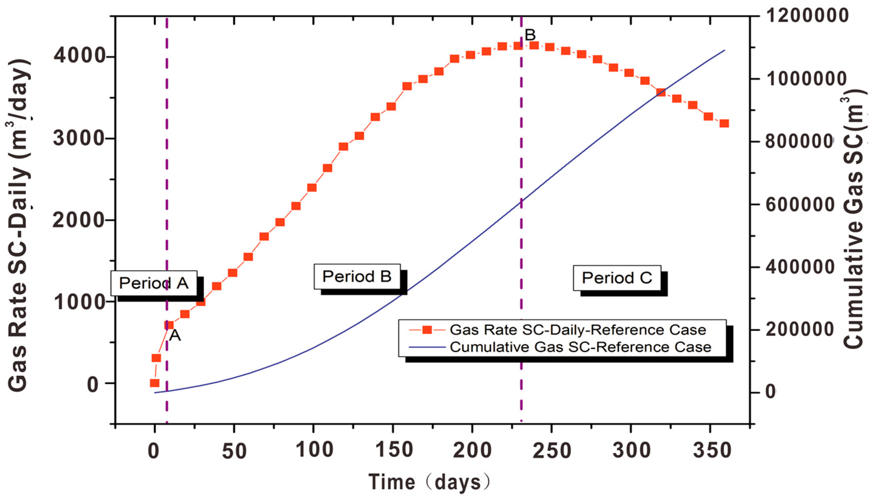
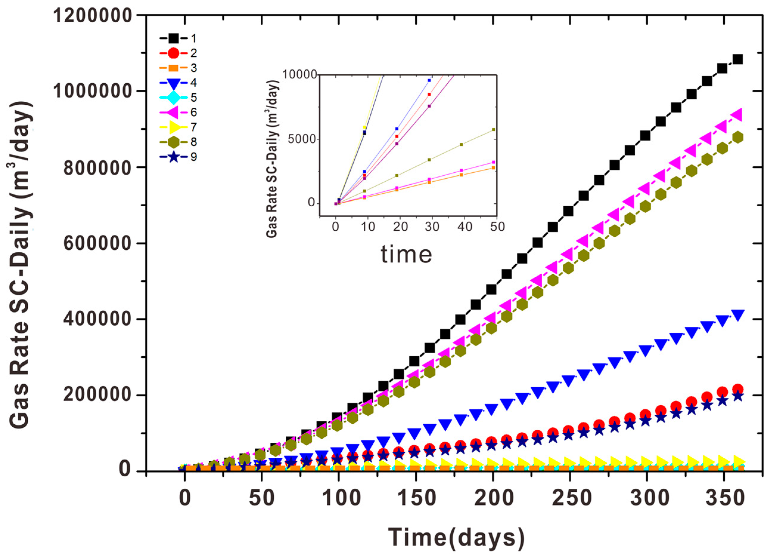
(1): As for the actual geological model of the Shenhu area, the gas accumulation of the basis scenario of operational conditions with 1000 m well spacing, 3000 kPa BHP and perforated 4–13 intervals can reach 1.02 × 10⁶ S Tm³ after one years’ production, and the peak daily gas rate can reach approximately 4000 STm³/day. That outcome can be used as reference data when it comes to the real field development.
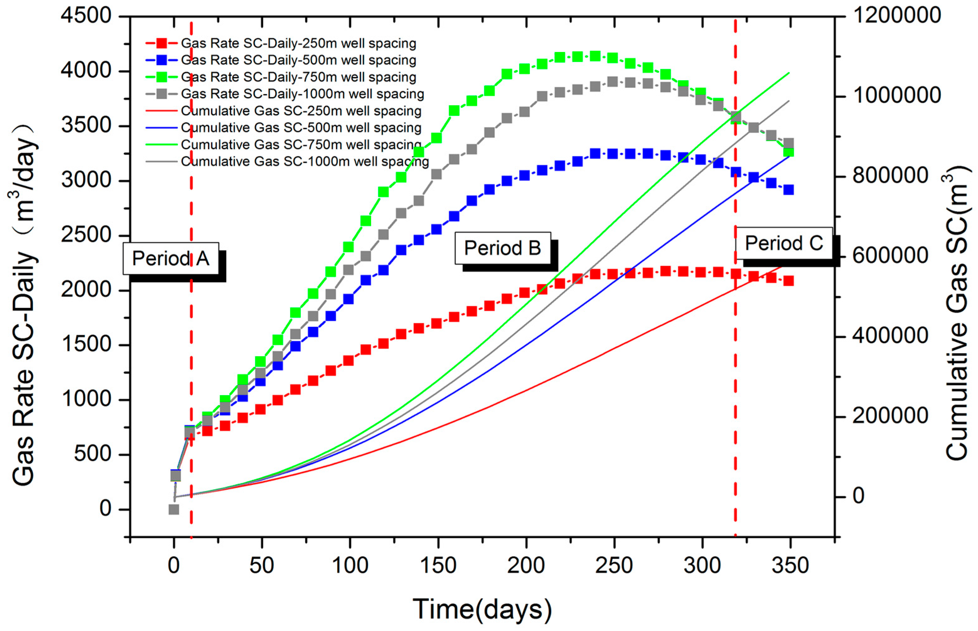
(2): The operation conditions indeed have an important influence on the production performance. The well spacing analysis indicates that the total production period can be divided into three periods according to the degrees of the influencing factors that are initial period, interacting & storage period and storage period. Different well spacing acts similarly in period A because of the pressure interaction has not happened, the pressure dropdown waves and the controlling storage work together in the period B, and the controlling storage plays the main role in the following period when the pressure interaction is slight after the long production time.
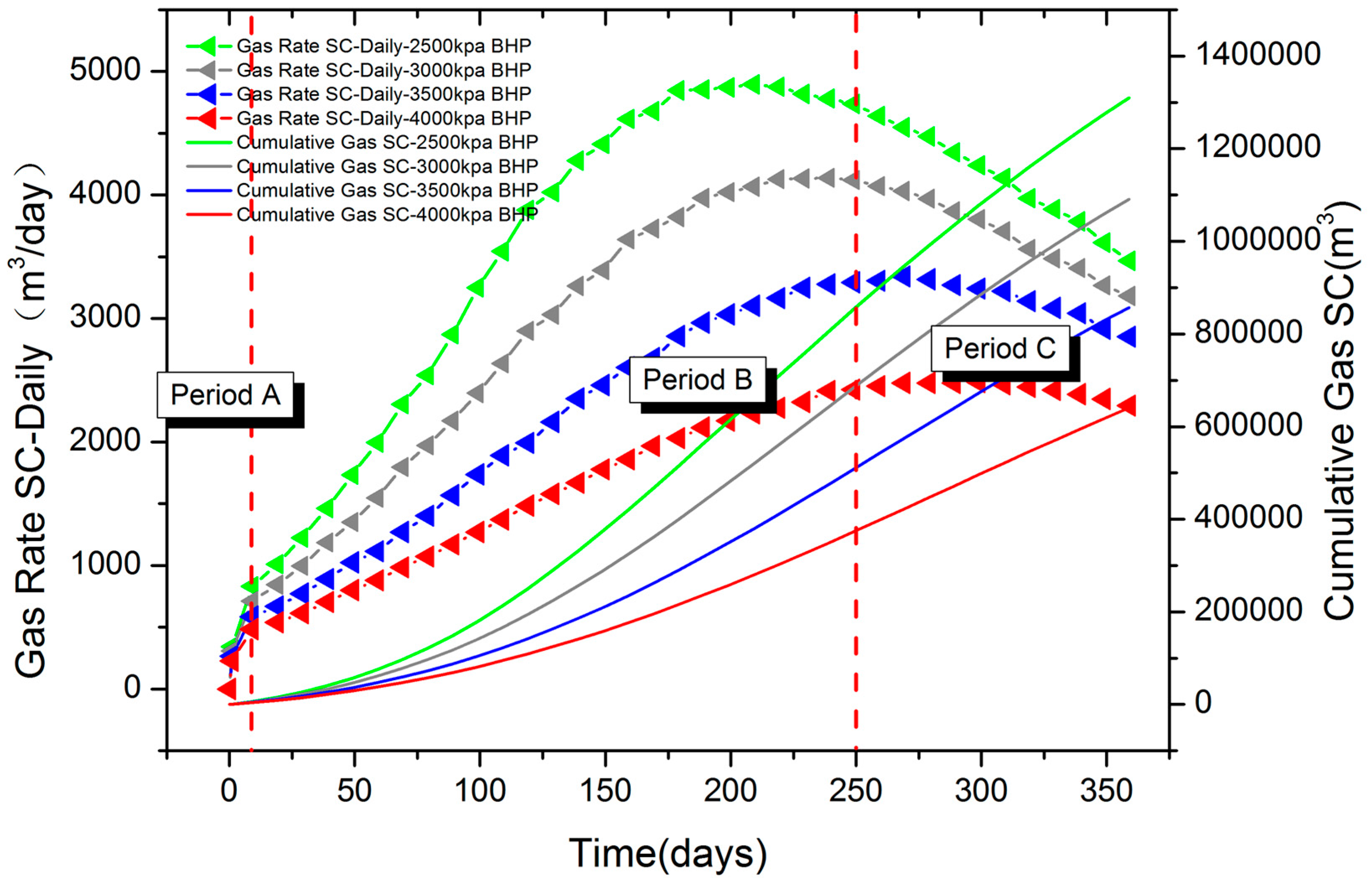
(3): The BHP analysis indicates that the total production period can also be divided into three periods according to the size of pressure gap that are initial period, speeding period and declining period. Different BHP reflects different pressure gaps between the hydrate reservoir and the BHP, that is the driving force which subsequently results in a higher gas travel velocity in the host formation which subsequently in turn stimulates even more hydrate dissociation. In the following decades, when the gap is gone, the reaction will remain in phase equilibrium and no more extra gas will be produced.
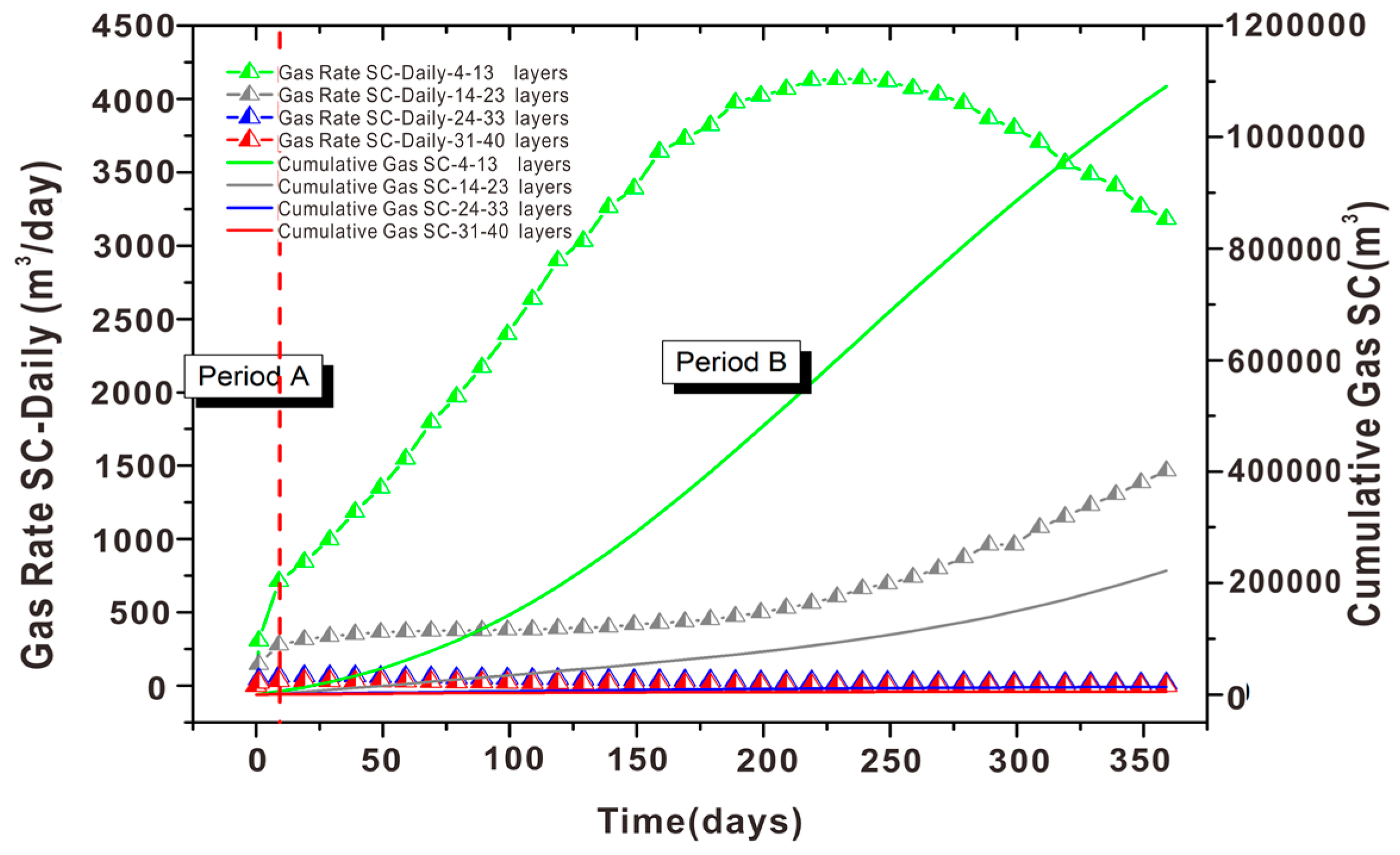
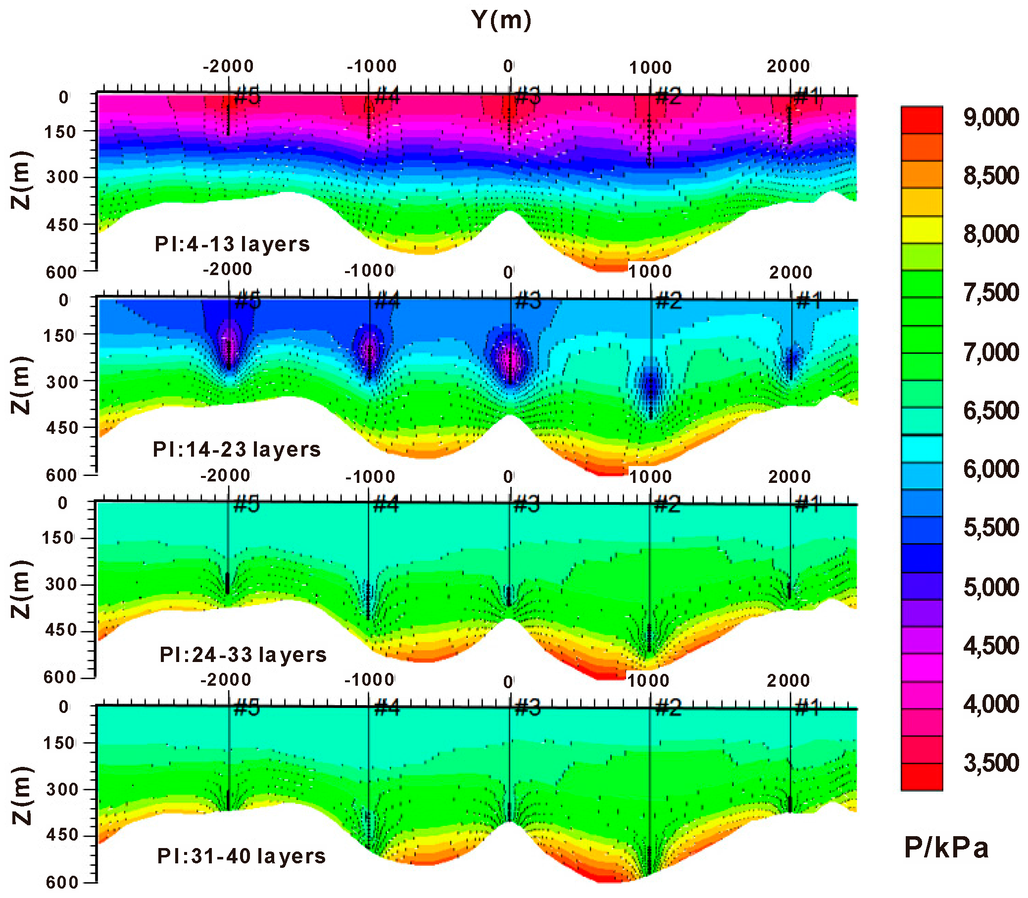
(4): The perforation intervals analysis indicates that the pressure around the perforated layers is so dominant that lower pressure in the hydrate deposit produced more gas than other scenarios. The perforation intervals have an extremely strong effect on the production. The production well perforation interval should be located in the upper deposit in the development of the Shenhu case.
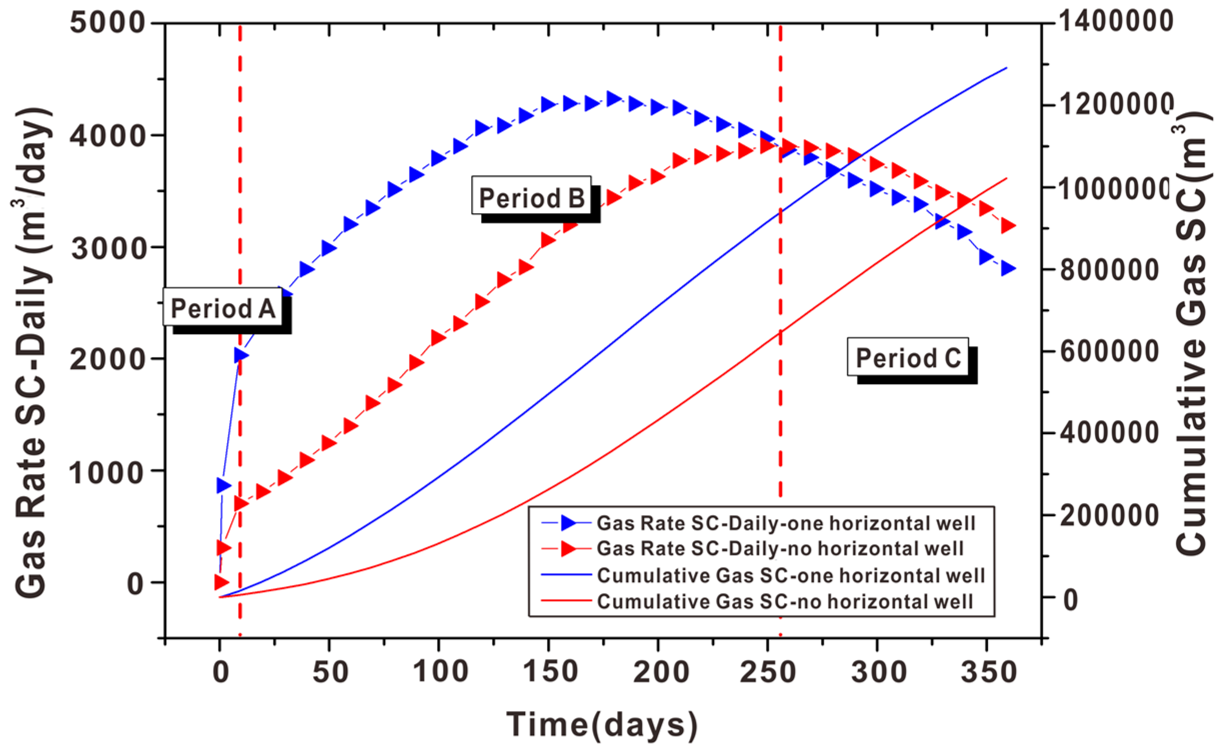
(5): The well type analysis indicates the use of horizontal wells in such reservoirs may not be attractive in the long run as all layers showed an upward gas migration block which is contrary to gas production from conventional gas reservoirs.
(6): One factor at a time design and orthogonal design indicate that the order of the effects of the factors on gas yield was perforation intervals > bottom hole pressure > well spacing.

Acknowledgments

This study was jointly funded by the National Science Foundation for Young Scientists of China (No. 51404291&41502131), Fundamental Research Funds for the Central Universities (NO. 14CX05024A), Shandong Natural Science Foundation (NO. ZR2013EEQ031&ZR2013DL011) and Key Laboratory of Natural Gas Hydrate of the Ministry of Land and Resources opening fund (SHW[2014]-DX-11). Thanks are due to GRID-Arendal for the generous permission that our manuscript features the graphic as Figure 1. We are grateful to all staff involved in this project, and also wish to thank the journal editors and the reviewers whose constructive comments improved the quality of this paper greatly.

Author Contributions

Zhixue Sun, Ying Xin, Qiang Sun and Shuhuan Lv conceived and designed the experiments; Zhixue Sun, Ying Xin and Qiang Sun created the geological model; Ruolong Ma and Jianguang Zhang provided several analysis methods; Qiang Sun and Ying Xin analyzed the result; Zhixue Sun contributed analysis tools; Qiang Sun wrote the manuscript; Shuhuan Lv, Mingyu Cai and Haoxuan Wang make a great contribution to the revision of manuscript.

Conflicts of Interest

The authors declare there is no conflicts of interest regarding the publication of this paper. The founding sponsors had no role in the design of the study; in the collection, analyses, or interpretation of data; in the writing of the manuscript, and in the decision to publish the results.

Appendix A

Governing Equations

The governing equations involved in the model includes three parts: kinetics of dissociation, heat transfer and multiphase fluid flow in porous media which will control the rate mechanisms and the CH₄ production from gas hydrates.

Mass balance for CH₄:

\frac{\partial (ρ_{g} v_{g x})}{\partial x} - \frac{\partial (ρ_{g} v_{g y})}{\partial y} - \frac{\partial (ρ_{g} v_{g z})}{\partial z} + g_{g} = \frac{\partial (ϕ ρ_{g} v_{g})}{\partial t}

(A1)

where ρ is the gas density; v is the velocity, g is the mass generation rate and ϕ is the porosity.

Mass balance for water:

\frac{\partial (ρ_{w} v_{w x})}{\partial x} - \frac{\partial (ρ_{w} v_{w y})}{\partial y} - \frac{\partial (ρ_{w} v_{w z})}{\partial z} + g_{w} = \frac{\partial (ϕ ρ_{w} v_{w})}{\partial t}

(A2)

Mass balance for CH₄-hydrate:

{\overset{•}{g}}_{H} = \frac{\partial (ϕ ρ_{H} S_{H})}{\partial t}

(A3)

where S is the saturation, t is the time.

The following equations describe fluid flow velocities:

The velocity along the I-direction for gas:

v_{g x} = \frac{κ κ_{r g}}{μ_{g}} \frac{\partial P_{g}}{\partial x}

(A4)

where κ is the absolute permeability, κ_r is the relative permeability, P is the pressure and μ is the viscosity.

The velocity along the J-direction for gas:

v_{g y} = \frac{κ κ_{r g}}{μ_{g}} \frac{\partial P_{g}}{\partial y}

(A5)

The velocity along the K-direction for gas:

v_{g z} = - \frac{κ κ_{r g}}{μ_{g}} \frac{\partial (P_{g} - γ_{g} z)}{\partial z}

(A6)

where γ is the fluid gravity.

The velocity along the I-direction for water:

v_{w x} = \frac{κ κ_{r w}}{μ_{w}} \frac{\partial P_{w}}{\partial x}

(A7)

The velocity along the J-direction for water:

v_{w y} = \frac{κ κ_{r w}}{μ_{w}} \frac{\partial P_{w}}{\partial y}

(A8)

The velocity along the K-direction for water:

v_{w z} = - \frac{κ κ_{r w}}{μ_{w}} \frac{\partial (P_{w} - γ_{w} z)}{\partial z}

(A9)

{\overset{•}{g}}_{g}

,

{\overset{•}{g}}_{w}

and

{\overset{•}{g}}_{H}

represent the rates of gas and water production and the hydrate dissociation rate, and are calculated by the Kim-Bishnoi model [46]:

{\overset{•}{g}}_{g} = k_{d} M_{g} A_{d e c} (f_{e} - f)

(A10)

where k_d is the decomposition rate constant, M is the molecular mass, A_dec is the hydrate surface area per unit volume and f is the fugacity:

{\overset{•}{g}}_{w} = 5.75 {\overset{•}{g}}_{g} \frac{M_{w}}{M_{g}}

(A11)

{\overset{•}{g}}_{H} = - {\overset{•}{g}}_{g} \frac{M_{H}}{M_{g}}

(A12)

The following equations describe the energy balance:

[\begin{array}{l} \frac{\partial}{\partial x} (k \frac{\partial T}{\partial x}) \\ + \frac{\partial}{\partial y} (k \frac{\partial T}{\partial y}) \\ + \frac{\partial}{\partial z} (k \frac{\partial T}{\partial z}) \end{array}] - [\begin{array}{l} \frac{\partial}{\partial x} (ρ_{g} v_{g x} h_{g} + ρ_{w} v_{w x} h_{w}) \\ + \frac{\partial}{\partial y} (ρ_{g} v_{g y} h_{g} + ρ_{w} v_{w y} h_{w}) \\ + \frac{\partial}{\partial z} (ρ_{g} v_{g z} h_{g} + ρ_{w} v_{w z} h_{w}) \end{array}] + {\overset{•}{Q}}_{H} + {\overset{•}{Q}}_{in} = \frac{\partial}{\partial t} [(1 - ϕ) ρ_{R} u_{R} + ϕ S_{H} ρ_{H} u_{H} + ϕ S_{g} ρ_{g} u_{g} + ϕ S_{w} ρ_{w} u_{w}]

(A13)

where k is the thermal conductivity, T is the temperature, h is the specific enthalpy. Q_H is the heat of hydrate decomposition unit bulk volume and Q_in is the direct heat input bulk volume:

and : {\overset{•}{Q}}_{H} = \frac{{\overset{•}{g}}_{H}}{M_{H}} Δ H_{R}

(A14)

where ΔH_R is the heat of reaction.

The kinetics of methane hydrate dissociation follows the Kim-Bishnoi model [46] as mentioned before. The value for the heat of dissociation is taken from Liu et al. [47].

- \frac{1}{V} \frac{d n_{{CH}_{4} - hyd}}{d t} = k_{d} A_{d e c} (f_{e} - f_{C H_{4}}); Δ H_{R} = 54.7 kJ / mol

(A15)

where V is the volume:

k_{d} = {k_{d}}^{0} \exp (\frac{- E}{R T})

(A16)

where E is activation energy, R is the universal gas constant.

Clarke and Bishnoi determined the kinetic parameters (

{k_{d}}^{0}, E

) by experiment. The fugacity of methane can be calculated as:

f_{{CH}_{4}} = φ P

;

f_{e} = φ P_{e}

for pure components. In addition, we have to assign

φ = 1

, since STARS does not allow fugacity calculations and the system is assumed to behave like an ideal gas:

- \frac{1}{V} \frac{d n_{{CH}_{4} - hyd}}{d t} = {k_{d}}^{0} \exp (\frac{- E}{R T}) (ϕ_{f} S_{H} A_{S H}) (ϕ_{f} S_{W}) (P_{e} - P_{CH 4})

(A17)

where

{k_{d}}^{0}

is the intrinsic decomposition rate constant.

Abbreviations

The following abbreviations are used in this manuscript:

$ρ_{g}$	gas density (g/cm³)
$ρ_{w}$	water density (g/cm³)
$ρ_{H}$	hydrate density (g/cm³)
$v_{g x}$	gas velocity along the x-axis (m/s)
$v_{g y}$	gas velocity along the y-axis (m/s)
$v_{g z}$	gas velocity along the z-axis (m/s)
$v_{g}$	gas velocity (m/s)
$v_{w}$	water velocity (m/s)
$v_{H}$	hydrate velocity (m/s)
x, y, z	Cartesian coordinates (m)
$g_{g}$	rate of gas production (g/(s·cm³))
$g_{w}$	rate of water production (g/(s·cm³))
$g_{H}$	rate of hydrate dissociation (g/(s·cm³))
ϕ	porosity
$S_{g}$	gas saturation
$S_{w}$	water saturation
$S_{H}$	hydrate saturation
t	time (days)
k	absolute permeability (μm²)
k_r	relative permeability (μm²)
k_eff	effective permeability (μm²)
P	pressure (kPa)
P_i	initial pressure (kPa)
$p_{w f}$	bottom hole pressure (kPa)
$μ_{g}$	gas viscosity (mPa·s)
$μ_{w}$	water viscosity (mPa·s)
$γ_{g}$	gas gravity (kN·m³)
$γ_{w}$	water gravity (kN·m³)
$k_{d}$	decomposition rate constant (g/(cm²·Pa·s))
$k_{d}^{0}$	intrinsic decomposition rate constant (g/(cm²·Pa·s))
M	molecular mass (kg/mol)
$A_{d e c}$	hydrate surface area per unit volume (cm²)
f	fugacity (kPa)
$f_{{CH}_{4}}$	fugacity of methane (kPa)
$f_{e}$	fugacity of pure components (kPa)
k	thermal conductivity
T	temperature (°C)
T_i	initial temperature (°C)
h	specific enthalpy
Q_H	heat of hydrate decomposition unit bulk volume (J)
Q_in	direct heat input bulk volume (J)
ΔH_R	heat of reaction (J)
V	volume (m³)
E	activation energy (kJ/mol)
R	universal gas constant (8.31 J/(mol·K))
A	reaction frequency factor
C	volumetric heat capacity (J/(m³·C))
m	geothermal gradient (K/m)
$λ_{R}$	thermal conductivity of the rock (J/(m·day·C))
d	well spacing (m)

References

Montzka, S.A.; Dlugokencky, E.J.; Butler, J.H. Non-CO₂ greenhouse gases and climate change. Nature 2011, 476, 43–50. [Google Scholar] [CrossRef] [PubMed]
Chu, S.; Majumdar, A. Opportunities and challenges for a sustainable energy future. Nature 2012, 488, 294–303. [Google Scholar] [CrossRef] [PubMed]
Lu, H.; Seo, Y.; Lee, J.; Moudrakovski, I.; Ripmeester, J.A.; Chapman, N.R.; Coffin, R.B.; Gardner, G.; Pohlman, J. Complex gas hydrate from the Cascadia margin. Nature 2007, 445, 303–306. [Google Scholar] [CrossRef] [PubMed]
Falenty, A.; Hansen, T.C.; Kuhs, W.F. Formation and properties of ice XVI obtained by emptying a type sII clathrate hydrate. Nature 2014, 516, 231–233. [Google Scholar] [CrossRef] [PubMed]
Sloan, E.D. Fundamental principles and applications of natural gas hydrates. Nature 2003, 426, 353–363. [Google Scholar] [CrossRef] [PubMed]
Sloan, E.D., Jr.; Koh, C. Clathrate Hydrates of Natural Gases; CRC Press: Boca Raton, FL, USA, 2007. [Google Scholar]
Johnson, A.H. Global Resource Potential of Gas Hydrate—A New Calculation. In Proceedings of the 7th International Conference on Gas Hydrates, Edinburgh, UK, 17–21 July 2011.
Zhong, D.L.; Daraboina, N.; Englezos, P. Recovery of CH₄ from coal mine model gas mixture (CH₄N₂) by hydrate crystallization in the presence of cyclopentane. Fuel 2013, 106, 425–430. [Google Scholar] [CrossRef]
Linga, P.; Daraboina, N.; Ripmeester, J.A.; Englezos, P. Enhanced rate of gas hydrate formation in a fixed bed column filled with sand compared to a stirred vessel. Chem. Eng. Sci. 2012, 68, 617–623. [Google Scholar] [CrossRef]
Zhong, D.; Ye, Y.; Yang, C.; Bian, Y.; Ding, K. Experimental investigation of methane separation from low-concentration coal mine gas (CH₄/N₂/O₂) by tetra-n-butyl ammonium bromide semiclathrate hydrate crystallization. Ind. Eng. Chem. Res. 2012, 51, 14806–14813. [Google Scholar] [CrossRef]
Zhong, D.; Englezos, P. Methane separation from coal mine methane gas by tetra-n-butyl ammonium bromide semiclathrate hydrate formation. Energy Fuels 2012, 26, 2098–2106. [Google Scholar] [CrossRef]
Kamath, V.A.; Godbole, S.P. Evaluation of hot-brine stimulation technique for gas production from natural gas hydrates. J. Pet. Technol. 1987, 39, 1379–1388. [Google Scholar] [CrossRef]
Zhao, J.; Cheng, C.; Song, Y.; Song, Y.; Liu, W.; Liu, Y.; Xue, K.; Zhu, Z.; Yang, Z.; Wang, D.; et al. Heat transfer analysis of methane hydrate sediment dissociation in a closed reactor by a thermal method. Energies 2012, 5, 1292–1308. [Google Scholar] [CrossRef]
Kawamura, T.; Ohtake, M.; Sakamoto, Y.; Haneda, H.; Komai, T.; Higuchi, S. Experimental Study on Steam Injection Method Using Methane Hydrate Core Samples. In Proceedings of the Seventh ISOPE Ocean Mining Symposium, Lisbon, Portugal, 1–6 July 2007; International Society of Offshore and Polar Engineers: Houston, TX, USA, 2007. [Google Scholar]
Li, G.; Moridis, G.J.; Zhang, K.; Li, X.-S. Evaluation of gas production potential from marine gas hydrate deposits in Shenhu area of South China Sea. Energy Fuels 2010, 24, 6018–6033. [Google Scholar] [CrossRef]
Li, X.S.; Li, B.; Li, G. Numerical simulation of gas production potential from permafrost hydrate deposits by huff and puff method in a single horizontal well in Qilian Mountain, Qinghai province. Energy 2012, 40, 59–75. [Google Scholar] [CrossRef]
Jiang, X.; Li, S.; Zhang, L. Sensitivity analysis of gas production from Class I hydrate reservoir by depressurization. Energy 2012, 39, 281–285. [Google Scholar] [CrossRef]
Collett, T.S. Gas hydrates as a future energy resource. Geotimes 2004, 49, 24–27. [Google Scholar]
Li, G.; Li, X.S.; Tang, L.G.; Zhang, Y. Experimental investigation of production behavior of methane hydrate under ethylene glycol injection in unconsolidated sediment. Energy Fuels 2007, 21, 3388–3393. [Google Scholar] [CrossRef]
Sun, D.; Englezos, P. Storage of CO₂ in a partially water saturated porous medium at gas hydrate formation conditions. Int. J. Greenh. Gas Control 2014, 25, 1–8. [Google Scholar] [CrossRef]
Graue, A.; Ersland, G.; Birkedal, K.A.; Hauge, L. Methane Production from Natural Gas Hydrates by CO₂ Replacement-Review of Lab Experiments and Field Trial. In Proceedings of the SPE Bergen One Day Seminar, Bergen, Norway, 2 April 2014; Society of Petroleum Engineers: Houston, TX, USA, 2014. [Google Scholar]
Kurihara, M.; Funatsu, K.; Ouchi, H.; Masuda, Y.; Narita, H. Investigation on Applicability of Methane Hydrate Production Methods to Reservoirs with Diverse Characteristics. In Proceedings of the 5th International Conference on Gas Hydrates, Trondheim, Norway, 13–16 July 2005.
Moridis, G.J. Toward Production from Gas Hydrates: Current Status, Assessment of Resources, and Simulation-Based Evaluation of Technology and Potential; Lawrence Berkeley National Laboratory: Berkeley, CA, USA, 2008. [Google Scholar]
Li, G.; Li, B.; Li, X.-S.; Zhang, Y.; Wang, Y. Experimental and numerical studies on gas production from methane hydrate in porous media by depressurization in pilot-scale hydrate simulator. Energy Fuels 2012, 26, 6300–6310. [Google Scholar] [CrossRef]
Moridis, G.J.; Reagan, M.T. Strategies for Gas Production from Oceanic Class 3 Hydrate Accumulations; Lawrence Berkeley National Laboratory: Berkeley, CA, USA, 2007. [Google Scholar]
Sloan, E.D.; Koh, C.A. Clathrate Hydrates of Natural Gases, 3rd ed.; CRC Press: Boca Raton, FL, USA, 2008; p. 119. [Google Scholar]
Moridis, G.J. The Use of Horizontal Wells in Gas Production from Hydrate Accumulations; Lawrence Berkeley National Laboratory: Berkeley, CA, USA, 2008. [Google Scholar]
Wang, Y.; Li, X.-S.; Li, G.; Zhang, Y.; Li, B.; Chen, Z.-Y. Experimental investigation into methane hydrate production during three-dimensional thermal stimulation with five-spot well system. Appl. Energy 2013, 110, 90–97. [Google Scholar] [CrossRef]
Uddin, M.; Coombe, D.; Wright, F. Modeling of CO₂-hydrate formation in geological reservoirs by injection of CO₂ gas. J. Energy Resour. Technol. 2008, 130, 032502. [Google Scholar] [CrossRef]
Howe, S.J. Production Modeling and Economic Evaluation of a Potential Gas Hydrate Pilot Production Program on the North Slope of Alaska; University of Alaska: Fairbanks, AK, USA, 2004. [Google Scholar]
Uddin, M.; Wright, F.; Coombe, D. Numerical study of gas evolution and transport behaviours in natural gas-hydrate reservoirs. J. Can. Pet. Technol. 2011, 50, 70–88. [Google Scholar] [CrossRef]
Hong, H.; Pooladi-Darvish, M.; Bishnoi, P.R. Analytical modelling of gas production from hydrates in porous media. J. Can. Pet. Technol. 2003, 42, 45–56. [Google Scholar] [CrossRef]
Moridis, G.J. TOUGH + HYDRATE v1. 2 User’s Manual: A Code for the Simulation of System Behavior in Hydrate-Bearing Geologic Media; Lawrence Berkeley National Laboratory: Berkeley, CA, USA, 2014. [Google Scholar]
White, M.D.; Wurstner, S.K.; McGrail, B.P. Numerical studies of methane production from Class 1 gas hydrate accumulations enhanced with carbon dioxide injection. Mar. Pet. Geol. 2011, 28, 546–560. [Google Scholar] [CrossRef]
Garapati, N. Reservoir Simulation for Production of CH₄ from Gas Hydrate Reservoirs Using CO₂/CO₂ + N₂ by HydrateResSim; West Virginia University: Morgantown, WV, USA, 2013. [Google Scholar]
Masuda, Y.; Yamamoto, K.; Tadaaki, S.; Ebinuma, T.; Nagakubo, S. Japan’s methane hydrate R&D program progresses to phase 2. Natl. Gas Oil 2012, 304, 285–4541. [Google Scholar]
Stars, C. Advanced Process and Thermal Reservoir Simulator; Computer Modelling Group Ltd.: Calgary, AB, Canada, 2008. [Google Scholar]
Su, Z.; Moridis, G.J.; Zhang, K.; Wu, N. A huff-and-puff production of gas hydrate deposits in Shenhu area of South China Sea through a vertical well. J. Pet. Sci. Eng. 2012, 86–87, 54–61. [Google Scholar] [CrossRef]
Li, G.; Moridis, G.J.; Zhang, K.; Li, X. Evaluation of Gas Production Potential from Marine Gas Hydrate Deposits in Shenhu Area of South China Sea. Energy Fuels 2010, 24, 6018–6033. [Google Scholar] [CrossRef]
Su, Z.; Cao, Y.; Wu, N.; Chen, D.; Yang, S.; Wang, H. Numerical investigation on methane hydrate accumulation in Shenhu Area, northern continental slope of South China Sea. Mar. Pet. Geol. 2012, 38, 158–165. [Google Scholar] [CrossRef]
Myshakin, E.; Gamwo, I.; Warzinski, R. Experimental Design Applied to Simulation of Gas Productivity Performance at Reservoir and Laboratory Scales Utilizing Factorial ANOVA Methodology. In Proceedings of the TOUGH Symposium, Berkeley, CA, USA, 14–16 September 2009.
Saltelli, A.; Ratto, M.; Andres, T.; Campolongo, F.; Cariboni, J.; Gatelli, D.; Saisana, M.; Tarantola, S. Global Sensitivity Analysis: The Primer; John Wiley & Sons: New York, NY, USA, 2008. [Google Scholar]
Friedmann, F.; Chawathe, A.; Larue, D.K. Assessing Uncertainty in Channelized Reservoirs Using Experimental Designs. In Proceedings of the SPE Annual Technical Conference and Exhibition, New Orleans, LA, USA, 30 September–3 October 2001.
White, C.D.; Royer, S.A. Experimental Design as a Framework for Reservoir Studies. In Proceedings of the SPE Reservoir Simulation Symposium, The Woodlands, TX, USA, 18–20 February 2013.
Montgomery, D.C. Design and Analysis of Experiments; John Wiley & Sons: New York, NY, USA, 2008. [Google Scholar]
Kim, H.; Bishnoi, P.; Heidemann, R.; Rizvi, S. Kinetics of methane hydrate decomposition. Chem. Eng. Sci. 1987, 42, 1645–1653. [Google Scholar] [CrossRef]
Liu, Y.; Strumendo, M.; Arastoopour, H. Simulation of methane production from hydrates by depressurization and thermal stimulation. Ind. Eng. Chem. Res. 2008, 48, 2451–2464. [Google Scholar] [CrossRef]

Figure 1. Gas hydrate resource potential by global region, adapted from Johnson [7], with permission from GRID-Arendal, 2015.

Figure 2. The mechanism of the three main methods to develop hydrate reservoirs. (A) Thermal Stimulation; (B) Depressurization; (C) Inhibitor Injection.

Figure 3. The mechanism for changing the pressure or the temperature conditions to destroy the stability of the original equilibrium and cause a phase change.

Figure 4. A map showing the location of the study area, drilling sites, and the confirmed gas hydrate distribution in the Shenhu area.

Figure 5. The distribution of permeability of an actual geological model on the northern continental slope of the South China Sea.

Figure 6. The volumetric rate of daily gas production and the cumulative gas production of reference case in one years’ simulation.

Figure 7. The evolution of spatial distribution of S_g during gas production from the methane hydrate deposit at some site of the Shenhu Area, South China Sea.

Figure 8. The evolution of spatial distribution of S_h during gas production from the methane hydrate deposit at some site of the Shenhu Area, South China Sea.

Figure 9. The evolution of spatial distribution of T during gas production from the methane hydrate deposit at some site of the Shenhu Area, South China Sea.

Figure 10. The evolution of spatial distribution of P during gas production from the methane hydrate deposit at some site of the Shenhu Area, South China Sea.

Figure 11. The volumetric rate of daily gas production and the cumulative gas production of four scenarios with different well spacing in one years’ simulation.

Figure 12. The volumetric rate of daily gas production and the cumulative gas production of four scenarios with different BHP in one years’ simulation.

Figure 13. The pressure contrast of final moments with different well type.

Figure 14. The volumetric rate of daily gas production and the cumulative gas production of two scenarios with different well type in one years’ simulation.

Figure 15. The volumetric rate of daily gas production and the cumulative gas production of two scenarios with different perforation intervals in one years’ simulation.

Figure 16. The pressure contrast of final moments with different perforation intervals.

Figure 17. The cumulative gas production of the orthogonal design experiment.

Table 1. Summary of main simulation model parameters were used in the model.

**Table 1.** Summary of main simulation model parameters were used in the model.
Basic Properties	Symbols	Value	Units
Intrinsic porosity (all formations)	ϕ	0.059–0.143	-
Mean porosity	$\bar{ϕ}$	0.083
Intrinsic permeability (all formations)	k	1.53–31.43	md
Mean permeability	$\bar{k}$	17.73	md
Grain density (all formations)	ρ	2600	kg/m³
Well spacing	d	1000	m
Bottom hole pressure	p_wf	3000	kPa
Well type	-	vertical
Perforated intervals	-	4–13	layer
Thermal conductivity of the rock	λ_R	1.5 × 10⁵	J/(m·day·C)
Volumetric heat capacity	C	8 × 10⁵	J/(m³·C)
Initial Pressure	p_i	1000	kPa
Initial Temperature	T_i	10	°C
Gas saturation	S_g	0.02	-
Gas composition	-	100% CH₄
Geothermal gradient	m	0.0433	K/m
Water saturation	S_w	0.98	-
Water salinity (mass fraction)	S‰	0.0305
Hydrate concentration	-	4616	gmole/m³
Reaction frequency factor	A	1.097 × 10¹³	-
Activation energy	E	89,660	J/mole
Enthalpy	H	51,858	J/mole

Table 2. Summary of the changing factor and its range.

**Table 2.** Summary of the changing factor and its range.
Operational Factor	Well Spacing (WS)/m	Bottom Hole Pressure (BHP)/kPa	Perforated Intervals (PI)/Layer	Well Type (WP)
Value Range	1000	2500	4–13	5 vertical wells
	750	3000	14–23	3 vertical wells + 1 horizontal wells
	500	3500	24–33
	250	4000	31–40

Table 3. The basic data of the orthogonal design experiment and sensitive factor analysis. L (3³).

**Table 3.** The basic data of the orthogonal design experiment and sensitive factor analysis. L (3³).
Case No.	Well Spacing/m	BHP/kPa	Perforated Intervals/Layer	Cumulative Gas/m³
1	1000	2500	4–13	1,083,475
2	1000	3000	14–23	214,946
3	1000	3500	24–33	12,142
4	750	2500	14–23	414,221
5	750	3000	24–33	14,024
6	750	3500	4–13	937,339
7	500	2500	24–33	25,048
8	500	3000	4–13	878,382
9	500	3500	14–33	198,471
Mean A	436,854.33	507,581.33	966,398.67
Mean B	455,194.67	369,117.33	275,879.33
Mean C	367,300.33	382,650.66	74,879.00
Range	87,894.333	124,930.66	891,519.67
Better level	A2	B1	C1	1,309,742
Order	3	2	1

© 2016 by the authors; licensee MDPI, Basel, Switzerland. This article is an open access article distributed under the terms and conditions of the Creative Commons Attribution (CC-BY) license (http://creativecommons.org/licenses/by/4.0/).

Share and Cite

MDPI and ACS Style

Sun, Z.; Xin, Y.; Sun, Q.; Ma, R.; Zhang, J.; Lv, S.; Cai, M.; Wang, H. Numerical Simulation of the Depressurization Process of a Natural Gas Hydrate Reservoir: An Attempt at Optimization of Field Operational Factors with Multiple Wells in a Real 3D Geological Model. Energies 2016, 9, 714. https://doi.org/10.3390/en9090714

AMA Style

Sun Z, Xin Y, Sun Q, Ma R, Zhang J, Lv S, Cai M, Wang H. Numerical Simulation of the Depressurization Process of a Natural Gas Hydrate Reservoir: An Attempt at Optimization of Field Operational Factors with Multiple Wells in a Real 3D Geological Model. Energies. 2016; 9(9):714. https://doi.org/10.3390/en9090714

Chicago/Turabian Style

Sun, Zhixue, Ying Xin, Qiang Sun, Ruolong Ma, Jianguang Zhang, Shuhuan Lv, Mingyu Cai, and Haoxuan Wang. 2016. "Numerical Simulation of the Depressurization Process of a Natural Gas Hydrate Reservoir: An Attempt at Optimization of Field Operational Factors with Multiple Wells in a Real 3D Geological Model" Energies 9, no. 9: 714. https://doi.org/10.3390/en9090714

Note that from the first issue of 2016, this journal uses article numbers instead of page numbers. See further details here.

Article Menu

Numerical Simulation of the Depressurization Process of a Natural Gas Hydrate Reservoir: An Attempt at Optimization of Field Operational Factors with Multiple Wells in a Real 3D Geological Model

Abstract

1. Introduction

1.1. Background

1.2. Status Quo in Hydrate Reservoir Modeling

1.3. Objectives

2. Geological Model and Simulation Scenarios

2.1. Geological Settings and Real Model

2.2. Reservoir Parameters and Component Setting

2.3. Scenarios & Simulation

3. Production Performance from Some Sites in the Shenhu Area

3.1. Reference Case and Gas Production

3.2. Spatial Distribution of S_g and S_h

3.3. Spatial Distribution of T and P

4. Results and Discussion

4.1. Sensitivity of Producer Well Spacing

4.2. Sensitivity of BHP

4.3. Sensitivity of Well Types

4.4. Sensitivity of Perforation Intervals of Producing Well

4.5. Orthogonal Design

5. Conclusions

Acknowledgments

Author Contributions

Conflicts of Interest

Appendix A

Governing Equations

Abbreviations

References

Share and Cite

Article Metrics

Article Access Statistics

Further Information

Guidelines

MDPI Initiatives

Follow MDPI

Article Menu

Numerical Simulation of the Depressurization Process of a Natural Gas Hydrate Reservoir: An Attempt at Optimization of Field Operational Factors with Multiple Wells in a Real 3D Geological Model

Abstract

1. Introduction

1.1. Background

1.2. Status Quo in Hydrate Reservoir Modeling

1.3. Objectives

2. Geological Model and Simulation Scenarios

2.1. Geological Settings and Real Model

2.2. Reservoir Parameters and Component Setting

2.3. Scenarios & Simulation

3. Production Performance from Some Sites in the Shenhu Area

3.1. Reference Case and Gas Production

3.2. Spatial Distribution of Sg and Sh

3.3. Spatial Distribution of T and P

4. Results and Discussion

4.1. Sensitivity of Producer Well Spacing

4.2. Sensitivity of BHP

4.3. Sensitivity of Well Types

4.4. Sensitivity of Perforation Intervals of Producing Well

4.5. Orthogonal Design

5. Conclusions

Acknowledgments

Author Contributions

Conflicts of Interest

Appendix A

Governing Equations

Abbreviations

References

Share and Cite

Article Metrics

Article Access Statistics

Further Information

Guidelines

MDPI Initiatives

Follow MDPI

3.2. Spatial Distribution of S_g and S_h