Radial Force-Current Characteristics Analysis of Three-Pole Radial-Axial Hybrid Magnetic Bearings and Their Structure Improvement

Abstract

The radial stator of three-pole radial-axial hybrid magnetic bearings (HMB) has three magnetic poles and the three magnetic poles are driven by a three-phase converter, so the three-pole radial-axial HMB has the advantages of compact structure, low cost, low power consumption and so on. However, as the sum of three-phase current is zero and the three radial magnetic poles are asymmetric, the relationship between the radial suspension force and the control current is nonlinear. In this paper, firstly a mathematical model of three-pole radial-axial HMB is built based on the equivalent magnetic circuit method. The radial force-current characteristics are then analyzed based on the non-linearized model. The calculation, finite element method (FEM) and experimental results show that the suspension force on the x-axis is a quadratic function of the control current, but the suspension force on the y-axis is linear with control current. Besides, the suspension forces on the two radial axes are coupled with each other. Then, in order to decrease the nonlinearity and coupling of radial force-current characteristics, the six-pole radial-axial HMB is proposed based on the above analyses. The radial force-current characteristics of the six-pole radial-axial HMB are also analyzed based on the non-linearitzed model and are validated by 3-D FEM analysis. The calculation and FEM results have shown that the radial force-current relationship of a six-pole radial-axial HMB is linear and there is no coupling between the two radial axes.

1. Introduction

Magnetic bearings suspend the rotor in space by magnetic force, there is no friction between rotor and stator, so they have the advantages of no-wear, no-lubrication, low power loss, long service life and so on [1]. Their high performance has made magnetic bearings be used in the area of space, energy storage flywheels, high speed electrical spindles, turbine machines, life sciences and so on [2,3,4,5,6].

Magnetic bearings can be classified into active magnetic bearings (AMBs) [7], passive magnetic bearing (PMBs) [8] and hybrid magnetic bearing (HMBs) [9], according to the way the suspension force is generated. According to the displacement direction of the rotor controlled by a magnetic bearing, it can be classified into an axial magnetic bearing [10], a radial magnetic bearing [11] or a radial-axial magnetic bearing [12]. The radial magnetic bearing usually has four or eight magnetic poles, but the three-pole magnetic bearings are proposed to simplify the structure, improve the space utilization and reduce the volume and cost of the power amplifier. In [13], a three-pole AMB driven by two power amplifiers is proposed. The three magnetic poles are arranged in a Y-shape, where the upper two magnetic poles share a same bias current and control current, and the lower magnetic pole is driven by another control current. This kind of structure can reduce the power amplifier needed but the fluxes in the three magnetic poles are coupled with each other, so it is not easy to control. In [14], the three-pole AMB is driven by three power amplifiers, so the magnetic forces of the three poles are controlled independently, and the force control is relatively easy. However the cost and power consumption of three power amplifiers are high.

Compared with power amplifiers, the three-phase converter driving technology is mature, low cost and low power consumption, so it is more suitable for three-pole magnetic bearings. In [15], a three-pair pole AMB driven by a three-phase converter is proposed and it is proposed that the bias flux is necessary for three-phase converters driving three-pole magnetic bearings. In [16], the three-pole AMB is driven by a three-phase converter, but the bias flux is not balanced in the three magnetic poles. The unbalanced bias flux causes an unbalanced force which can be used to overcome the mass of the rotor. However, the unbalanced bias flux makes the force-current relationship nonlinear, and the control is difficult. In [17], according to the high nonlinearity of the three-pole AMB without bias flux, the feedback linearization method is used and the pole-displacement control and robust control are investigated based on the previous feedback linearization. In [18], a double stator slice structured three-pole HMB are proposed. Each stator slice has three magnetic poles, and a permanent magnet between two stator slices generates the bias flux. Besides, the magnetic bearing is driven by a three-phase converter. As the permanent magnet replaces the bias coils and the control coils are driven by three-phase converter, it has relatively low power consumption. In [19], the mathematical model of a three-pole HMB was built by the Maxwell tensor method. In [20], the edge effect was considered when modeling the three-pole HMB to improve the accuracy of the model. In [21], the three-phase six-pole magnetic bearing is investigated. The stator has three poles wound with coils and three poles embedded with permanent magnets to generated bias flux. Compared with the traditional eight pole magnetic bearings, the power loss is very small. In [22], the three-pole radial-axial HMB is proposed. The radial stator has three poles and is driven by a three-phase converter, and a permanent magnet provides both radial and axial bias flux. As the radial and axial displacement can be controlled by adjusting the axial and radial control currents, respectively, the radial magnetic bearing and axial magnetic bearing are combined into one magnetic bearing. The axial length of magnetic bearings is reduced, which can improve the critical speed of rotor. The utilization of a permanent magnet and three-phase converter reduces the power consumption and cost of the magnetic bearing, so the three-pole radial-axial HMB has wide application prospects [23].

In [24], the design process of a three-pole radial-axial HMB was introduced and the suspension force characteristics were analyzed based on the mathematical model, but the analysis did not consider the saturated flux density of iron, so the results did not correspond to the actual situation. In [25], the radial and axial carrying capacities of three-pole radial-axial HMB were analyzed by finite element analysis, but the force-current characteristics were not analyzed. In [26], an improved model of a three-pole radial-axial HMB was proposed, but the model only considered the linear part of suspension force. In [27], the linear model and nonlinear model were compared with the experimental results, and the two models were not completely coincident with the experimental results, so the “switching model” was proposed to make the model more accurate. However, the force-current characteristics are only analyzed when the control current is positive and the forces on x-axis and y-axis were not analyzed separately. Although the above references have presented some studies on three-pole radial-axial HMBs, the nonlinearity between radial force and control current were not analyzed in detail and the reasons behind the generation of the nonlinearity were not analyzed.

Although the three-pole radial-axial HMB has many advantages, the radial suspension force-current characteristics are influenced by the factor that three radial poles are not completely symmetrical about the coordinate axis and the sum of the three phase currents is zero. In this paper, a mathematical model of three-pole radial-axial HMB is firstly built based on the equivalent magnetic circuit. Then the radial force-current characteristics are analyzed based on the non-linearized model and the assumption that the rotor is in the center position. Next the reasons for the nonlinearity generation and coupling are analyzed. The finite element method (FEM) and experiment results have validated the correctness of the analytical results. Based on the above analyses, a six-pole radial-axial HMB is proposed to reduce the nonlinearity and coupling of the radial suspension force. The radial force-current characteristics are analyzed based on the equivalent magnetic circuit method and FEM. Compared with the three-pole radial-axial HMB, the radial force-current relationship of the six-pole radial-axial HMB possesses better linearity and there is almost no coupling.

2. Radial Suspension Force-Current Characteristics Analysis of the Three-Pole Radial-Axial Hybrid Magnetic Bearings (HMB)

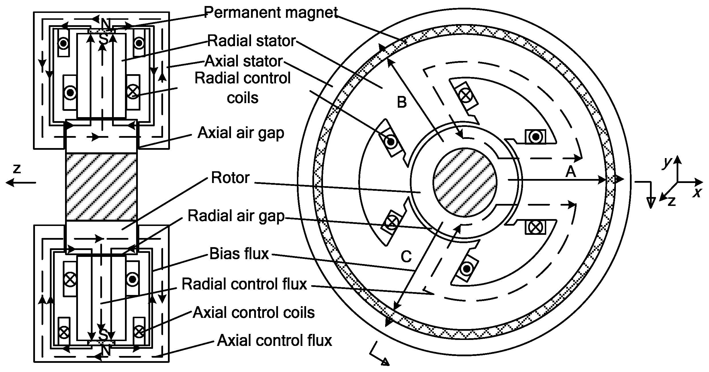
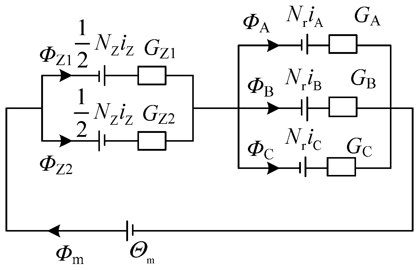
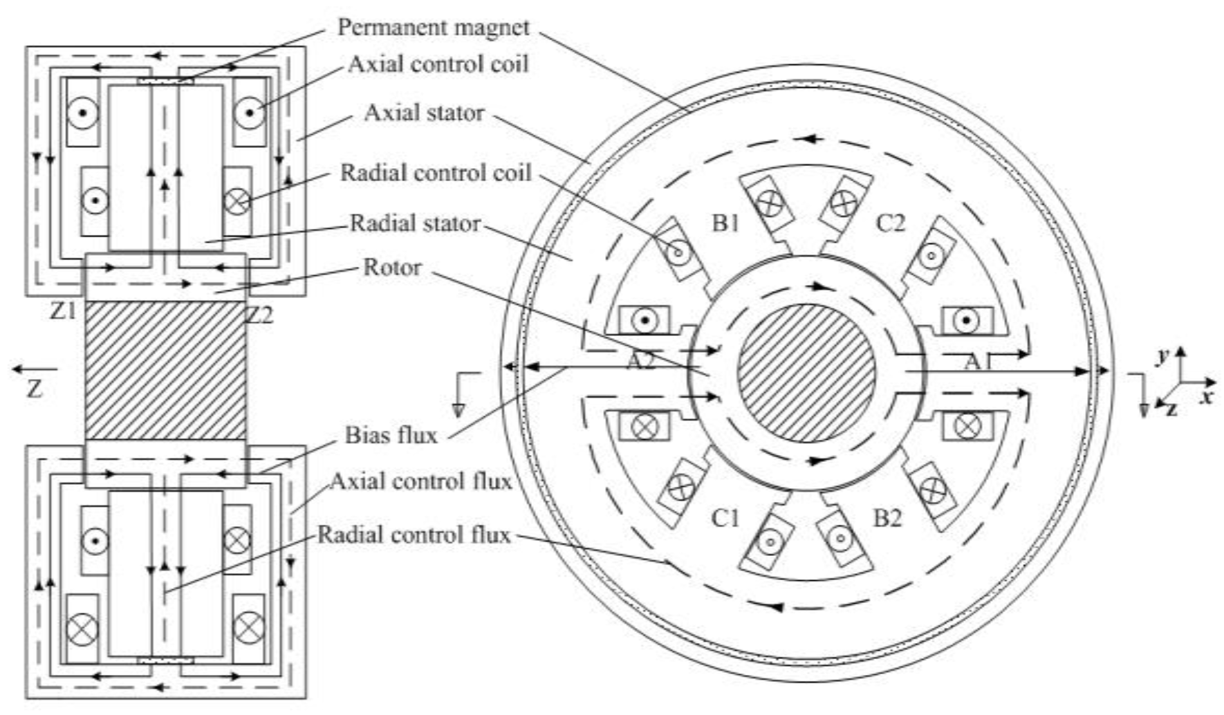
2.1. Mathematical Model of the Three-Pole Radial-Axial Hybrid Magnetic Bearings (HMB)

The three-pole radial-axial HMB consists of a rotor, radial stator, axial stator, permanent magnet, radial control coils and axial control coils, as shown in Figure 1.

Neglecting the flux leakage and reluctance of iron, the corresponding mathematical model can be obtained by the equivalent magnetic circuit method. The equivalent magnetic circuit can be obtained according to the flux paths in Figure 1, as shown in Figure 2.

In Figure 2, the Θ_m is the equivalent magnetomotive force of permanent magnet, Φ_m is the total bias flux, Φ_Z1, Φ_Z2 are the fluxes in the left and right air gaps, respectively, Φ_A, Φ_B, Φ_C are the fluxes in three radial air gaps, N_Z is the sum turns of the axial control coils in the two sides, N_r is the turns of the coil turned on each radial magnetic pole, i_Z is the axial control current, i_A, i_B, i_C are the currents in the three radial control coils, G_Z1, G_Z2 are the permeance of the axial air gaps, G_A, G_B, G_C are the permeance of the radial air gaps. The permeance of the air gaps can be expressed as:

$$\begin{array}{l}{G}_{\mathrm{Z}1}=\frac{{\mu }_0{S}_{\mathrm{Z}}}{{\delta }_{\mathrm{Z}}-z},G_{\mathrm{Z}2}=\frac{{\mu }_0{S}_{\mathrm{Z}}}{{\delta }_{\mathrm{Z}}+z},G_{\mathrm{A}}=\frac{{\mu }_0{S}_{\mathrm{r}}}{{\delta }_{\mathrm{r}}-x}\\ G_{\mathrm{B}}=\frac{{\mu }_0{S}_{\mathrm{r}}}{{\delta }_{\mathrm{r}}+\frac{1}{2}x-\frac{\sqrt{3}}{2}y},G_{\mathrm{C}}=\frac{{\mu }_0{S}_{\mathrm{r}}}{{\delta }_{\mathrm{r}}+\frac{1}{2}x+\frac{\sqrt{3}}{2}y}\end{array}$$

(1)

where, μ₀ is the permeanbility of vacuum, S_Z is the area of the axial magnetic pole, S_r is the area of the radial magnetic pole, δ_Z, δ_r are the axial and radial air gap lengths, respectively, when the rotor is in the center, z is the eccentric displacement of the rotor in the axial direction, x, y are the radial eccentric displacements of the rotor.

According to Figure 2, the fluxes in the axial and radial air gaps can be obtained by Gauss’s law:

$$\{\begin{array}{l}{\Phi }_{\mathrm{Z}1}=\frac{\left({\Theta }_{\mathrm{m}}+\frac{1}{2}{N}_{\mathrm{Z}}{i}_{\mathrm{Z}}\right)G_{\mathrm{r}}+N_{\mathrm{Z}}{i}_{\mathrm{Z}}{G}_{\mathrm{Z}2}+{\Phi }_{\mathrm{rc}}}{G_{\mathrm{sum}}}{G}_{\mathrm{Z}1}\\ {\Phi }_{\mathrm{Z}2}=\frac{\left({\Theta }_{\mathrm{m}}-\frac{1}{2}{N}_{\mathrm{Z}}{i}_{\mathrm{Z}}\right)G_{\mathrm{r}}-N_{\mathrm{Z}}{i}_{\mathrm{Z}}{G}_{\mathrm{Z}1}+{\Phi }_{\mathrm{rc}}}{G_{\mathrm{sum}}}{G}_{\mathrm{Z}2}\\ {\Phi }_{\mathrm{A}}=\frac{\left({\Theta }_{\mathrm{m}}+N_{\mathrm{r}}{i}_{\mathrm{A}}\right)G_{\mathrm{ZS}}+\frac{1}{2}{N}_{\mathrm{Z}}{i}_{\mathrm{Z}}{G}_{\mathrm{Z}\mathrm{M}}+N_{\mathrm{r}}{i}_{\mathrm{A}}{G}_{\mathrm{r}}-{\Phi }_{\mathrm{rc}}}{G_{\mathrm{sum}}}{G}_{\mathrm{A}}\\ {\Phi }_{\mathrm{B}}=\frac{\left({\Theta }_{\mathrm{m}}+N_{\mathrm{r}}{i}_{\mathrm{B}}\right)G_{\mathrm{Z}\mathrm{S}}+\frac{1}{2}{N}_{\mathrm{Z}}{i}_{\mathrm{Z}}{G}_{\mathrm{Z}\mathrm{M}}+N_{\mathrm{r}}{i}_{\mathrm{B}}{G}_{\mathrm{r}}-{\Phi }_{\mathrm{rc}}}{G_{\mathrm{sum}}}{G}_{\mathrm{B}}\\ {\Phi }_{\mathrm{C}}=\frac{\left({\Theta }_{\mathrm{m}}+N_{\mathrm{r}}{i}_{\mathrm{C}}\right)G_{\mathrm{Z}\mathrm{S}}+\frac{1}{2}{N}_{\mathrm{Z}}{i}_{\mathrm{Z}}{G}_{\mathrm{Z}\mathrm{M}}+N_{\mathrm{r}}{i}_{\mathrm{C}}{G}_{\mathrm{r}}-{\Phi }_{\mathrm{rc}}}{G_{\mathrm{sum}}}{G}_{\mathrm{C}}\end{array}$$

(2)

where, G_sum = G_Z1 + G_Z2 + G_A + G_B + G_C, G_r = G_A + G_B + G_C, G_ZS = G_Z1 + G_Z2, G_ZM = G_Z1 − G_Z2, Φ_rc = N_r(i_AG_A + i_BG_B + i_CG_C).

According to the relationship between magnetic force and flux: F = Φ²/2μ₀S, the axial and radial suspension force can be obtained:

$$F_j=\frac{{{\Phi }_j}^2}{2{\mu }_0{S}_j}(j=\mathrm{Z}1,\mathrm{Z}2,\mathrm{A},\mathrm{B},\mathrm{C})$$

(3)

2.2. Radial Force-Current Characteristics Analysis

As this paper only discusses the relationship between the radial suspension force and the control current, the rotor is assumed to be in the center position, so the permeance of the axial air gaps in the left and right side are the same (G_Z1 = G_Z2 = G_Z0) and the permeance of the three radial air gaps are the same (G_A = G_B = G_C = G_r0). Therefore Equation (2) can be simplified as:

$$\{\begin{array}{l}{\Phi }_{\mathrm{Z}1}={\Phi }_{\mathrm{Z}0}+k_{i\mathrm{Z}}{i}_{\mathrm{Z}},{\Phi }_{\mathrm{Z}2}={\Phi }_{\mathrm{Z}0}-k_{i\mathrm{Z}}{i}_{\mathrm{Z}}\\ {\Phi }_{\mathrm{A}}={\Phi }_{\mathrm{r}0}+k_{\mathrm{ir}}{i}_{\mathrm{A}},{\Phi }_{\mathrm{B}}={\Phi }_{\mathrm{r}0}+k_{\mathrm{ir}}{i}_{\mathrm{B}},{\Phi }_{\mathrm{C}}={\Phi }_{\mathrm{r}0}+k_{\mathrm{ir}}{i}_{\mathrm{C}}\end{array}$$

(4)

where, ${\Phi }_{Z0}=\frac{3{\Theta }_{\mathrm{m}}{G}_{\mathrm{r}0}{G}_{Z0}}{3G_{\mathrm{r}0}+2G_{Z0}}$, $k_{i\mathrm{Z}}=\frac{1}{2}{N}_{\mathrm{Z}}{G}_{\mathrm{Z}0}$ ${\Phi }_{\mathrm{r}0}=\frac{2{\Theta }_{\mathrm{m}}{G}_{Z0}{G}_{\mathrm{r}0}}{3G_{\mathrm{r}0}+2G_{Z0}}$, $k_{i\mathrm{r}}=N_r{G}_{r0}$.

2.2.1. Radial Carrying Capacity Analysis

When designing magnetic bearings, the saturated flux density B_S should be set so as to avoid magnetic saturation in the iron. When the flux density in the air gaps reaches the settled saturated flux density, the current in the control coils reaches a maximum value. Taking the A-phase magnetic pole as an example, when the current in the A-phase control coils is maximum (i_rmax), the flux density in the A-phase air gap is B_S, which can be expressed as:

$${\Phi }_{\mathrm{Amax}}={\Phi }_{\mathrm{r}0}+k_{\mathrm{ir}}{i}_{\mathrm{rmax}}=B_{\mathrm{S}}{S}_{\mathrm{r}}$$

(5)

No matter how the flux direction flows through the air gap, the suspension force is only attractive force and no repulsive force, so when the control current in the A-phase coil is negative maximum (−i_rmax), the minimum suspension force in the direction of magnetic poles is generated, namely zero, which can be expressed as:

$${\Phi }_{\mathrm{Amin}}={\Phi }_{\mathrm{r}0}-k_{\mathrm{ir}}{i}_{\mathrm{rmax}}=0$$

(6)

Solving Equations (5) and (6), it can be obtained that:

$${\Phi }_{\mathrm{r}0}=k_{\mathrm{ir}}{i}_{\mathrm{rmax}}=0.5B_{\mathrm{S}}{S}_{\mathrm{r}}$$

(7)

In the rectangular coordinate system shown in Figure 1, the x-axis is along with the A-phase magnetic pole, the B-phase magnetic pole is in the negative part of the x-axis and positive part of the y-axis, the C-phase magnetic pole is in the negative part of the x-axis and the negative y-axis. The phase difference between the three radial magnetic poles is 120°. The condition of generating maximum suspension force in the direction of the x-axis and y-axis can be analyzed as follows:

When the suspension force is max on the positive x-axis, the A-pole should generate the maximum force and the flux reaches saturated flux density. Besides, as the B-pole and C-pole are in the negative part of the x-axis, the force of the B-pole and C-pole should be min, namely zero. Under this condition, the current in the A-pole should be maximum (i_rmax) and the current in the B-pole and C-pole should be negative maximum (−i_rmax), but for a three-phase converter driving three-pole magnetic bearings, the sum of the three-phase current should be zero. However, the sum of the three-phase current is −i_rmax under the above conditions generating the maximum suspension force on the positive x-axis, which cannot be realized by the three-phase converter. For this reason, the carrying capacities in different directions of the coordinate axis are different.

In order to satisfy the requirement that the sum of the three-phase current is zero and the force generated by the B-pole and C-pole is as small as possible, the current of the B-pole and C-pole should be −0.5i_rmax. In this condition, the flux in the three radial air gaps can be calculated:

$$\{\begin{array}{l}{\Phi }_{\mathrm{A}}={\Phi }_{\mathrm{r}0}+k_{\mathrm{ir}}{i}_{\mathrm{rmax}}=B_{\mathrm{S}}{S}_{\mathrm{r}}\\ {\Phi }_{\mathrm{B}}={\Phi }_{\mathrm{r}0}-0.5k_{\mathrm{ir}}{i}_{\mathrm{rmax}}=0.25B_{\mathrm{S}}{S}_{\mathrm{r}}\\ {\Phi }_{\mathrm{C}}={\Phi }_{\mathrm{r}0}-0.5k_{\mathrm{ir}}{i}_{\mathrm{rmax}}=0.25B_{\mathrm{S}}{S}_{\mathrm{r}}\end{array}$$

(8)

Projecting the suspension force of the three radial magnetic poles onto the x-axis, the maximum suspension force on positive x-axis can be obtained:

$$F_{\mathrm{x}\max 1}=F_{\mathrm{A}}-\frac{1}{2}{F}_{\mathrm{B}}-\frac{1}{2}{F}_{\mathrm{C}}=\frac{15{B_{\mathrm{S}}}^2{S}_{\mathrm{r}}}{32{\mu }_0}$$

(9)

When the suspension force is max on the negative x-axis, the current of the A-pole should be negative max (−i_rmax) to generate the minimum force, namely zero. To satisfy the requirement that the sum of the three-phase current is zero, the current in the B-pole and C-pole should be half of the maximum value (0.5i_rmax). So the flux in three radial air gaps can be calculated:

$$\{\begin{array}{l}{\Phi }_{\mathrm{A}}={\Phi }_{\mathrm{r}0}-k_{\mathrm{ir}}{i}_{\mathrm{rmax}}=0\\ {\Phi }_{\mathrm{B}}={\Phi }_{\mathrm{r}0}+0.5k_{\mathrm{ir}}{i}_{\mathrm{rmax}}=0.75B_{\mathrm{S}}{S}_{\mathrm{r}}\\ {\Phi }_{\mathrm{C}}={\Phi }_{\mathrm{r}0}+0.5k_{\mathrm{ir}}{i}_{\mathrm{rmax}}=0.75B_{\mathrm{S}}{S}_{\mathrm{r}}\end{array}$$

(10)

The maximum suspension force on negative x-axis can be obtained:

$$F_{\mathrm{x}\max 2}=F_{\mathrm{A}}-\frac{1}{2}{F}_{\mathrm{B}}-\frac{1}{2}{F}_{\mathrm{C}}=-\frac{9{B_{\mathrm{S}}}^2{S}_{\mathrm{r}}}{32{\mu }_0}$$

(11)

When the suspension force on the y-axis is maximum, the current of the B-pole should be max (i_rmax) and the current of the C-pole should be negative max (−i_rmax). The current of the A-pole must be zero. In this condition, the fluxes in the three radial air gaps can be calculated:

$$\{\begin{array}{l}{\Phi }_{\mathrm{A}}={\Phi }_{\mathrm{r}0}=0.5B_{\mathrm{S}}{S}_{\mathrm{r}}\\ {\Phi }_{\mathrm{B}}={\Phi }_{\mathrm{r}0}+k_{\mathrm{ir}}{i}_{\mathrm{rmax}}=B_{\mathrm{S}}{S}_{\mathrm{r}}\\ {\Phi }_{\mathrm{C}}={\Phi }_{\mathrm{r}0}-k_{\mathrm{ir}}{i}_{\mathrm{rmax}}=0\end{array}$$

(12)

Projecting the force of the three radial magnetic poles onto the y-axis, the maximum suspension force on the positive y-axis can be obtained:

$$F_{\mathrm{y}\max }=\frac{\sqrt{3}}{2}{F}_{\mathrm{B}}-\frac{\sqrt{3}}{2}{F}_{\mathrm{C}}=\frac{\sqrt{3}{B_{\mathrm{S}}}^2{S}_{\mathrm{r}}}{4{\mu }_0}$$

(13)

As the component force of the A-pole on the y-axis is zero, the suspension force on the y-axis only depends on the B-pole and C-pole. Besides, the B-pole and C-pole are symmetric about the x-axis, so the maximum forces on the positive y-axis and negative y-axis are the same.

Comparing Equations (9), (11) and (13), it can be seen that the carrying capacity in the different rectangular coordinate directions are different. The carrying capacity on the positive x-axis is max and on the negative x-axis it is min, but if we neglect the coordinate system and just consider the direction of the magnetic poles, it can be discovered that the carrying capacity in the direction along with the A-pole is max and in the opposite direction it is min. The situation is the same for the B-pole and C-pole.

2.2.2. Nonlinearity Analysis

As there are two controlled variables and three input currents, the three-phase current (i_A, i_B, i_C) should be equivalent to the two phase current (i_x, i_y) by Clark transformation:

$$\{\begin{array}{l}{i}_{\mathrm{x}}=\sqrt{\frac{2}{3}}\left(i_{\mathrm{A}}-\frac{1}{2}{i}_{\mathrm{B}}-\frac{1}{2}{i}_{\mathrm{C}}\right)\\ i_{\mathrm{y}}=\sqrt{\frac{2}{3}}\left(\frac{\sqrt{3}}{2}{i}_{\mathrm{B}}-\frac{\sqrt{3}}{2}{i}_{\mathrm{C}}\right)\end{array}$$

(14)

The relationship between suspension force on the x-axis F_x and control current i_x is first analyzed without considering the control current of i_y, so we make i_y = 0 and as the sum of three-phase current is zero, it can be obtained that i_B = i_C = −0.5i_A according to Equation (14). In this condition, the suspension force on the x-axis F_x and control current i_x can be calculated by:

$$F_{\mathrm{x}}=F_{\mathrm{A}}-\frac{1}{2}{F}_{\mathrm{B}}-\frac{1}{2}{F}_{\mathrm{C}}=\frac{k_{\mathrm{ir}}{i}_{\mathrm{x}}\left(2\sqrt{6}{\Phi }_{\mathrm{r}0}+k_{\mathrm{ir}}{i}_{\mathrm{x}}\right)}{4{\mu }_0{S}_r}$$

(15)

Then we make i_x = 0, which means i_A = 0 and i_B = −i_C according to (14), so the relationship between suspension force on y-axis F_y and control current i_y can be calculated by:

$$F_{\mathrm{y}}=\frac{\sqrt{3}}{2}{F}_{\mathrm{B}}-\frac{\sqrt{3}}{2}{F}_{\mathrm{C}}=\frac{\sqrt{6}}{2}\frac{{\Phi }_{\mathrm{r}0}{k}_{\mathrm{ir}}{i}_{\mathrm{y}}}{{\mu }_0{S}_r}$$

(16)

From Equations (15) and (16), it can be seen that when i_y = 0, the relationship between the suspension force on the x-axis F_x and control current i_x is not linear, even though the rotor is maintained in the center position. The F_x is a quadratic function of i_x, which causes the carrying capacity on the positive x-axis and negative x-axis to be different. However, when i_x = 0, the relationship between suspension force on the y-axis F_y and control current i_y is linear.

2.2.3. Coupling Analysis

According to Equation (4), the force generated by three radial magnetic poles can be calculated:

$$\{\begin{array}{l}{F}_{\mathrm{A}}=\frac{{{\Phi }_{\mathrm{r}0}}^2+2{\Phi }_{\mathrm{r}0}{k}_{\mathrm{ir}}{i}_{\mathrm{A}}+{k_{\mathrm{ir}}}^2{i_{\mathrm{A}}}^2}{2{\mu }_0{S}_{\mathrm{r}}}\\ F_{\mathrm{B}}=\frac{{{\Phi }_{\mathrm{r}0}}^2+2{\Phi }_{\mathrm{r}0}{k}_{\mathrm{ir}}{i}_{\mathrm{B}}+{k_{\mathrm{ir}}}^2{i_{\mathrm{B}}}^2}{2{\mu }_0{S}_{\mathrm{r}}}\\ F_{\mathrm{C}}=\frac{{{\Phi }_{\mathrm{r}0}}^2+2{\Phi }_{\mathrm{r}0}{k}_{\mathrm{ir}}{i}_{\mathrm{C}}+{k_{\mathrm{ir}}}^2{i_{\mathrm{C}}}^2}{2{\mu }_0{S}_{\mathrm{r}}}\end{array}$$

(17)

Projecting the force generated by the three radial magnetic poles onto the x-axis and y-axis, respectively, and transforming the three-phase current into two-phase current by the Clark transformation, the relationship between the radial suspension forces F_x, F_y and control currents i_x, i_y can be expressed by:

$$\{\begin{array}{l}{F}_{\mathrm{x}}=\frac{\sqrt{6}{\Phi }_{\mathrm{r}0}{k}_{\mathrm{ir}}{i}_{\mathrm{x}}+\frac{1}{2}{k_{\mathrm{ir}}}^2{i_{\mathrm{x}}}^2}{2{\mu }_0{S}_r}-\frac{\frac{1}{2}{k_{\mathrm{ir}}}^2{i_{\mathrm{y}}}^2}{2{\mu }_0{S}_r}\\ F_{\mathrm{y}}=\frac{\sqrt{6}{\Phi }_{\mathrm{r}0}{k}_{\mathrm{ir}}-{k_{\mathrm{ir}}}^2{i}_{\mathrm{x}}}{2{\mu }_0{S}_r}{i}_{\mathrm{y}}\end{array}$$

(18)

It can be seen from Equation (18) that without considering the rotor eccentricity, there is still coupling between the radial suspension force on the x-axis and y-axis. When i_y is constant, F_x is a quadratic function of i_x and when i_y changes, F_x decreases with the square of i_y. When i_x is constant, F_y is linear with i_y and when i_x changes, the slope of F_y − i_y curve decreases with i_x. These results are based on the rotor without eccentricity. If the eccentricity is considered, the nonlinearity and coupling between the suspension force on the x-axis and y-axis will be stronger.

2.3. Finite Element Analysis

In order to validate the above analyses, the parameters of a three-pole radial-axial HMB are designed based on the requirement of radial carrying capacity being 200 N. The parameters are listed in

Table 1. Parameters of three-pole radial-axial hybrid magnetic bearings (HMB).

Parameters	Value
Radial and axial air gap length δr, δZ/mm	0.5
Saturation flux density BS/T	0.8
The area of radial magnetic poles SrP/mm2	1396
The area of axial magnetic poles SZP/mm2	2094
The max ampere-turns of radial coils Nrirmax/At	160
The max ampere-turns of axial coils Nrirmax/At	320
Magnetomotive force of permanent magnet Θm/At	320
Outer diameter of rotor DRot1/mm	68
Inner diameter of rotor DRot2/mm	34
Axial width of rotor WRot/mm	39
Outer diameter of radial stator yoke Dr1/mm	149
Inner diameter of radial stator yoke Dr2/mm	115
Inner diameter of radial magnetic poles Dr3/mm	69
Radial width of radial magnetic poles WrP/mm	45
Axial width of radial stator LrP/mm	29
Outer diameter of permanent magnet Dmout/mm	155
Inner diameter of permanent magnet Dmin/mm	149
Axial width of permanent magnet Wm/mm	9.5
Outer diameter of axial magnetic poles DZP1/mm	65
Inner diameter of axial magnetic poles DZP2/mm	39
The width between axial magnetic poles WZP/mm	40
Inner width between axial stator discs WZS1/mm	50
Outer width between axial stator discs WZS2/mm	76
Outer diameter of axial stator cylinder DZS1/mm	170
Inner diameter of axial stator cylinder DZS2/mm	155

. The 3-D finite element model of the three-pole radial-axial HMB is built in the software ANSYS-Maxwell based on the design parameters. The finite element model is shown in Figure 3 and only the half of axial stator is shown for convenience of observation. Setting the excitation of i_x, i_y to both change from −1.22 A to 1.22 A, the finite element analysis results shown in Figure 4 are obtained.

Figure 4a is the curve between the suspension force on x-axis F_x and the control current i_x, i_y. It can be seen that when i_y is constant, the curve of F_x − i_x is a parabola, but when i_y changes, the curve moves down with the square of i_y, which is in agreement with the expression of F_x in Equation (18). Figure 4b is the curve between the suspension force on y-axis F_y and the control current i_x, i_y. It can be seen that when i_x is constant, the curve of F_y − i_y is a line, but when i_y changes the slope of F_y−i_y decrease with i_x, which is in agreement with the expression of F_y in Equation (18).

2.4. Experiment Validation

In order to validate the analysis, the radial suspension force-current characteristics are measured on a three-pole radial-axial HMB prototype as shown in Figure 5. The three-pole radial-axial HMB has been installed on one side of the iron cylinder. In order to measure the relationship between suspension force and control current, the following steps should be done: a current of 1 A is injected into the A-phase coils and currents of −0.5 A are injected into the B-phase and C-phase coils. Under this condition, the equivalent control current of i_x is 1.22 A and the rotor will be attracted on the backup bearing in the direction of the positive x-axis. Then we drag the rotor to the direction of the negative x-axis by a spring dynamometer. When the rotor is dragged to move, the value of spring dynamometer should be recorded. As the above analyses are based on the rotor without eccentricity, the force generated by rotor eccentricity should be decreased, so we move the rotor to the positive x-axis and on the backup bearing without injecting any currents, then drag the rotor by the spring dynamometer to the negative x-axis. When the rotor is dragged to move, the value of the dynamometer should be recorded. The force generated by the control current can be approximately regarded as the force generated by both the control current and rotor eccentricity reducing the force generated by rotor eccentricity. The suspension force on the x-axis can be measured by the above method when i_x is 1.22 A. Decreasing the current in the A-phase coil gradually and since the current in the B-phase, C-phase coil is negative half of the A-phase current (i_B = i_C = −0.5i_A), the relationship between suspension force on the x-axis F_x and control current i_x can be measured by the above method. Injecting different current values into the B-phase and C-phase coils and keeping i_B = −i_C, the relationship between the suspension force on y-axis F_y and control current i_y can be measured by the same method. The comparison of analytical, FEM and experiment results is shown in Figure 6.

Figure 6a is the relationship between the suspension force on the x-axis F_x and the control current i_x. Figure 6b is the relationship between the suspension force on the y-axis F_y and the control current i_y. It can be seen from Figure 6 that the experimental results are relatively lager than the analytical and FEM results. This is because the force measured in experiments is based on the rotor with eccentricity, although the force generated by rotor eccentricity is deduced, the approximate force generated by the current is still influenced by the eccentricity, so the measured suspension force generated by the control current is larger than the analytical and FEM results. However the curve trends of the suspension force on the x-axis and y-axis in the experimental results agrees very well with the analytical and FEM results. The curve of F_x − i_x is a parabola and the curve of F_y − i_y is a line, which validates the correction of the analytical results.

3. The Structure Improvement of Three-Pole Radial-Axial Hybrid Magnetic Bearings (HMB)

Comparing Equations (15), (16) with (18), it can be seen that Equations (15) and (16) represent a special situation of Equation (18), but when deducing Equations (15) and (16), the reason why the nonlinearity and coupling exist can be analyzed: as the suspension force is proportional to a quadratic function of the flux and the flux is proportional to the control current, the suspension force of each magnetic pole is proportional to the square of the current in the corresponding coil, so it is understandable that the suspension force on the x-axis F_x is a quadratic function of the control current i_x. However, the suspension force on the y-axis F_y is linear with the control current i_y. This is because when projecting the force of the B-pole and C-pole onto the y-axis, the quadratic items in the expression of the B-pole and C-pole magnetic force are the same and they cancel each other. As the suspension force on the y-axis only depends on the magnetic force of the B-pole and C-pole and the B-pole, C-pole are symmetric in the positive y-axis and negative y-axis, it can be deduced that the nonlinearity and coupling of the three-pole HMB radial suspension force can be decreased by the symmetrical structure, so if we add three magnetic poles in the opposite direction of the existing three radial magnetic poles, namely create a six-pole radial-axial HMB, the radial suspension force-current characteristics can be improved, so the six-pole radial-axial HMB is analyzed in the following section.

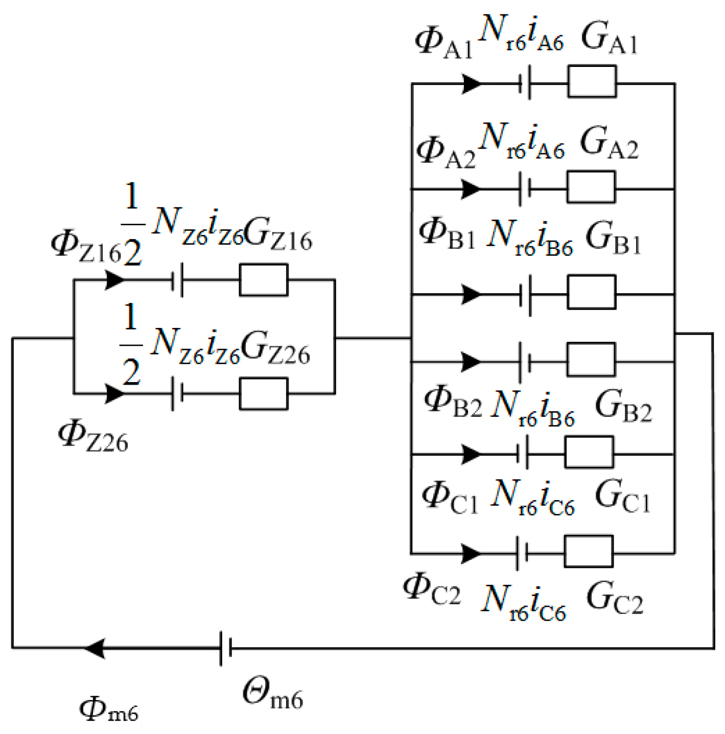
3.1. Radial Suspension Force-Current Characteristics Analysis of a Six-Pole Radial-Axial Hybrid Magnetic Bearings (HMB)

The structure and flux path of a six-pole radial-axial HMB is shown in Figure 7. The components of the six-pole radial-axial HMB are the same as those of the three-pole radial-axial HMB and the only difference is that the radial stator has six radial magnetic poles. The coils turned on two opposite radial magnetic poles are wound in the same direction and the control fluxes are in the same direction. As the bias flux in the two opposite radial magnetic poles are in opposite direction, the bias flux will increase with the control flux in one magnetic pole and decrease with the control flux in the opposite magnetic pole, which will generate the suspension force along with the radial magnetic pole. Besides, the opposite two radial coils are connected in series as one phase, so the six radial control coils are divided into a three-phase coil which is driven by one three-phase converter.

Neglecting the saturation, flux leakage, reluctance of stator and rotor, the equivalent flux circuit is analyzed as shown in Figure 8. In Figure 8, the θ_m6 is the equivalent magnetomotive force of the permanent magnet, Φ_m6 is the total bias flux, Φ_Z16, Φ_Z26 are the fluxes in the left and right air gaps, respectively, Φ_A1, Φ_B1, Φ_C1, Φ_A2, Φ_B2, Φ_C2 are the fluxes in the six radial air gaps, N_Z6 is the sum of turns of the axial control coils in the two sides, N_r6 is the turns of the coil turned on each radial magnetic pole, i_Z6 is the axial control current, i_A6, i_B6, i_C6 are the currents in the three radial control coils, G_Z16, G_Z26 are the permeances of the axial air gaps, G_A1, G_B1, G_C1, G_A2, G_B2, G_C2 are the permeances of radial air gaps. The permeance of the air gaps can be expressed as:

$$\begin{array}{l}{G}_{\mathrm{Z}16}=\frac{{\mu }_0{S}_{\mathrm{Z}6}}{{\delta }_{\mathrm{Z}6}-z},G_{\mathrm{Z}26}=\frac{{\mu }_0{S}_{\mathrm{Z}6}}{{\delta }_{\mathrm{Z}6}+z},G_{\mathrm{A}1}=\frac{{\mu }_0{S}_{\mathrm{r}6}}{{\delta }_{\mathrm{r}6}-x},G_{\mathrm{A}2}=\frac{{\mu }_0{S}_{\mathrm{r}6}}{{\delta }_{\mathrm{r}6}+x}\\ G_{\mathrm{B}1}=\frac{{\mu }_0{S}_{\mathrm{r}6}}{{\delta }_{\mathrm{r}6}+\frac{1}{2}x-\frac{\sqrt{3}}{2}y},G_{\mathrm{B}2}=\frac{{\mu }_0{S}_{\mathrm{r}6}}{{\delta }_{\mathrm{r}6}-\frac{1}{2}x+\frac{\sqrt{3}}{2}y}\\ G_{\mathrm{C}1}=\frac{{\mu }_0{S}_{\mathrm{r}6}}{{\delta }_{\mathrm{r}6}+\frac{1}{2}x+\frac{\sqrt{3}}{2}y},G_{\mathrm{C}2}=\frac{{\mu }_0{S}_{\mathrm{r}6}}{{\delta }_{\mathrm{r}6}-\frac{1}{2}x-\frac{\sqrt{3}}{2}y}\end{array}$$

(19)

where, μ₀ is the permeability of vacuum, S_Z6 is the area of the axial magnetic pole, S_r6 is the area of the radial magnetic pole, δ_Z6, δ_r6 are the axial and radial air gap lengths, respectively, when the rotor is in the center, z is the eccentric displacement of rotor in the axial direction, x, y are the radial eccentric displacements of the rotor.

According to Gauss’s law the expression of fluxes in axial and radial air gaps can be obtained:

$$\{\begin{array}{ll}{\Phi }_{\mathrm{Z}16}& =\frac{\left({\Theta }_{\mathrm{m}6}+\frac{1}{2}{N}_{\mathrm{Z}6}{i}_{\mathrm{Z}6}\right)G_{\mathrm{r}6}+N_{\mathrm{Z}6}{i}_{\mathrm{Z}6}{G}_{\mathrm{Z}26}+{\Phi }_{\mathrm{rc}6}}{G_{\mathrm{sum}6}}{G}_{\mathrm{Z}16}\\ {\Phi }_{\mathrm{Z}26}& =\frac{\left({\Theta }_{\mathrm{m}6}-\frac{1}{2}{N}_{\mathrm{Z}6}{i}_{\mathrm{Z}6}\right)G_{\mathrm{r}6}-N_{\mathrm{Z}6}{i}_{\mathrm{Z}6}{G}_{\mathrm{Z}16}+{\Phi }_{\mathrm{rc}6}}{G_{\mathrm{sum}6}}{G}_{\mathrm{Z}26}\\ {\Phi }_{j1}& =\frac{\left({\Theta }_{\mathrm{m}6}+N_{\mathrm{r}6}{i}_{j6}\right)G_{\mathrm{ZS}6}+\frac{1}{2}{N}_{\mathrm{Z}6}{i}_{\mathrm{Z}6}{G}_{\mathrm{ZM}6}}{G_{\mathrm{sum}6}}{G}_{j1}\\ & +\frac{N_{\mathrm{r}6}{i}_{j6}{G}_{\mathrm{r}6}-{\Phi }_{\mathrm{rc}6}}{G_{\mathrm{sum}6}}{G}_{j1}\\ {\Phi }_{j2}& =\frac{\left({\Theta }_{\mathrm{m}6}-N_{\mathrm{r}6}{i}_{j6}\right)G_{\mathrm{ZS}6}+\frac{1}{2}{N}_{\mathrm{Z}6}{i}_{\mathrm{Z}6}{G}_{\mathrm{ZM}6}}{G_{\mathrm{sum}6}}{G}_{j2}\\ & -\frac{N_{\mathrm{r}6}{i}_{j6}{G}_{\mathrm{r}6}-{\Phi }_{\mathrm{rc}6}}{G_{\mathrm{sum}6}}{G}_{j2}\\ & (j=\mathrm{A},\mathrm{B},\mathrm{C})\end{array}$$

(20)

where, $G_{\mathrm{ZS}6}=G_{\mathrm{Z}16}+G_{\mathrm{Z}26}$, $G_{\mathrm{ZM}6}=G_{\mathrm{Z}16}-G_{\mathrm{Z}26}$, $G_{\mathrm{r}6}=G_{\mathrm{A}1}+G_{\mathrm{A}2}+G_{\mathrm{B}1}+G_{\mathrm{B}2}+G_{\mathrm{C}1}+G_{\mathrm{C}2}$, $G_{\mathrm{sum}6}=G_{\mathrm{Z}1}+G_{\mathrm{Z}2}+G_{\mathrm{A}1}+G_{\mathrm{A}2}+G_{\mathrm{B}1}+G_{\mathrm{B}2}+G_{\mathrm{C}1}+G_{\mathrm{C}2}$, ${\Phi }_{\mathrm{rc}6}={\displaystyle \sum _{j=\mathrm{A},\mathrm{B},\mathrm{C}}{N}_{\mathrm{r}6}{i}_{j6}\left(G_{j1}-G_{j2}\right)}$.

The rotor is assumed to be in the center position for conveniently analyzing the relationship between the radial suspension force and control current. The permeances of the axial air gaps in the two sides are the same (G_Z16 = G_Z26 = G_Z06) and the permeances of the six radial air gaps are the same (G_A1 = G_A2 = G_B1 = G_B2 = G_C1 = G_C2 = G_r06). Then the expression of the fluxes in the six radial air gaps can be simplified as:

$$\{\begin{array}{l}{\Phi }_{j1}={\Phi }_{\mathrm{r}06}+k_{\mathrm{ir}6}{i}_{j6}\\ {\Phi }_{j2}={\Phi }_{\mathrm{r}06}-k_{\mathrm{ir}6}{i}_{j6}\end{array}(j=\mathrm{A},\mathrm{B},\mathrm{C})$$

(21)

where, ${\Phi }_{\mathrm{r}06}=\frac{2{\Theta }_{\mathrm{m}6}{G}_{Z06}{G}_{\mathrm{r}06}}{3G_{\mathrm{r}06}+2G_{Z06}}$, $k_{\mathrm{ir}6}=N_{\mathrm{r}6}{G}_{\mathrm{r}06}$.

According to the relationship between magnetic force and flux (F = Φ²/2μ₀S), the magnetic force of the six radial magnetic poles can be calculated. By projecting the six radial magnetic pole forces onto the x-axis and y-axis, respectively, the expression of the suspension force on the x-axis and y-axis can be obtained:

$$\{\begin{array}{ll}{F}_{\mathrm{x}}& =F_{\mathrm{A}1}-F_{\mathrm{A}2}-\frac{1}{2}{F}_{\mathrm{B}1}+\frac{1}{2}{F}_{\mathrm{B}2}-\frac{1}{2}{F}_{\mathrm{C}1}+\frac{1}{2}{F}_{\mathrm{C}2}\\ & =\frac{{\Phi }_{\mathrm{r}06}{k}_{\mathrm{ir}6}}{{\mu }_0{S}_{\mathrm{r}6}}\left(2i_{\mathrm{A}6}-i_{\mathrm{B}6}-i_{\mathrm{C}6}\right)\\ F_{\mathrm{y}}& =\frac{\sqrt{3}}{2}\left(F_{\mathrm{B}1}-F_{\mathrm{B}2}-F_{\mathrm{C}1}+F_{\mathrm{C}2}\right)\\ & =\frac{\sqrt{3}{\Phi }_{\mathrm{r}06}{k}_{\mathrm{ir}6}}{{\mu }_0{S}_{\mathrm{r}6}}\left(i_{\mathrm{B}6}-i_{\mathrm{C}6}\right)\end{array}$$

(22)

Transforming the three-phase current into two phase current by the Clark transformation, Equation (22) can be simplified as:

$$\{\begin{array}{c}{F}_{\mathrm{x}}=\frac{\sqrt{6}{\Phi }_{\mathrm{r}06}{k}_{\mathrm{ir}6}}{{\mu }_0{S}_{\mathrm{r}6}}{i}_{\mathrm{x}}\\ F_{\mathrm{y}}=\frac{\sqrt{6}{\Phi }_{\mathrm{r}06}{k}_{\mathrm{ir}6}}{{\mu }_0{S}_{\mathrm{r}6}}{i}_{\mathrm{y}}\end{array}$$

(23)

From Equation (23), it can be seen that the suspension forces on the x-axis and y-axis F_x, F_y are both linear with the control current i_x, i_y, respectively. The quadratic item in the expression of the suspension force and the coupling between suspension forces in the two directions of the radial axes are both eliminated compared with Equation (18), so the six-pole structure can improve the radial suspension force-current characteristics.

3.2. Validation by Finite Element Method (FEM) Analysis

To validate our analysis of the six-pole radial-axial HMB and compare it with the performance of a three-pole radial-axial HMB, a series of parameters are designed based on the requirement that the radial carrying capacity is the same with three-pole radial-axial HMB (200 N), as shown in

Table 2. Parameters of the six-pole radial-axial hybrid magnetic bearings (HMB).

Parameters	Value
Radial and axial air gap length δr, δZ/mm	0.5
Saturation flux density BS/T	0.8
The area of radial magnetic poles SrP/mm2	524
The area of axial magnetic poles SZP/mm2	1572
The max ampere-turns of radial coils Nrirmax/At	160
The max ampere-turns of axial coils Nrirmax/At	320
Magnetomotive force of permanent magnet Θm/At	320
Outer diameter of rotor DRot1/mm	77
Inner diameter of rotor DRot2/mm	39
Axial width of rotor WRot/mm	32
Outer diameter of radial stator yoke Dr1/mm	142
Inner diameter of radial stator yoke Dr2/mm	118
Inner diameter of radial magnetic poles Dr3/mm	82
Radial width of radial magnetic poles WrP/mm	78
Axial width of radial stator LrP/mm	22
Outer diameter of permanent magnet Dmout/mm	145
Inner diameter of permanent magnet Dmin/mm	142
Axial width of permanent magnet Wm/mm	10.5
Outer diameter of axial magnetic poles DZP1/mm	75
Inner diameter of axial magnetic poles DZP2/mm	60
The width between axial magnetic poles WZP/mm	33
Inner width between axial stator discs WZS1/mm	49
Inner diameter of axial stator cylinder DZS2/mm	145
Outer width between axial stator discs WZS2/mm	64
Outer diameter of axial stator cylinder DZS1/mm	153

. In Table 2, the outer diameter of the axial stator is 153 mm and the axial width of the axial stator is 64 mm, the volume of six-pole radial-axial HMB is 374,544 mm², however in Table 1, the outer diameter of the axial stator is 170 mm and the axial width of the axial stator is 76 mm, and the volume of three-pole radial-axial HMB is 549,100 mm². It can be easily seen that with the same radial carrying capacity, the volume of the six-pole radial-axial HMB is smaller than that of the three-pole radial-axial HMB.

The 3-D FEM model of six-pole radial-axial HMB is built in the FEM analysis software ANSYS-Maxwell as shown in Figure 9. For convenience of observation, the axial stator is cut along the xoz-plane and half of the axial stator is hidden.

Setting the control current of i_x and i_y changing from −1.22 A to 1.22 A, respectively, and calculating the three-phase current by inverse Clark transformation in ANSYS-Maxwell, the curve of the relationship between the radial suspension force and radial control current can be obtained as shown in Figure 10 and Figure 11. Figure 10 is the curve of the relationship between suspension force on the x-axis F_x and radial control current i_x, i_y. Figure 10a is the analytical results and Figure 10b is the FEM results. Figure 11 is the curve of the relationship between the suspension force on the y-axis F_y and the radial control current i_x, i_y. Figure 11a is the analytical results and Figure 11b is the FEM results. In Figure 10 and Figure 11, the FEM results are in great agreement with the analytical results: the suspension force on the x-axis is linear with i_x and the suspension force on the y-axis is linear with i_y, besides, there is no coupling between the suspension forces on the two radial coordinate axes, which validates the correctness of the analysis about the radial force-current characteristics of the six-pole radial-axial HMB.

4. Conclusions

In this paper, a mathematical model of a three-pole radial-axial HMB is first built by the equivalent magnetic circuit method. The radial force-current characteristics are analyzed based on the non-linearized model. The FEM and experiment results have validated the analyses. According to the analyses, the six-pole radial-axial HMB is proposed. The radial suspension force-current characteristics of the six-pole radial-axial HMB are analyzed. The following conclusions can be obtained based on the results:

(1)

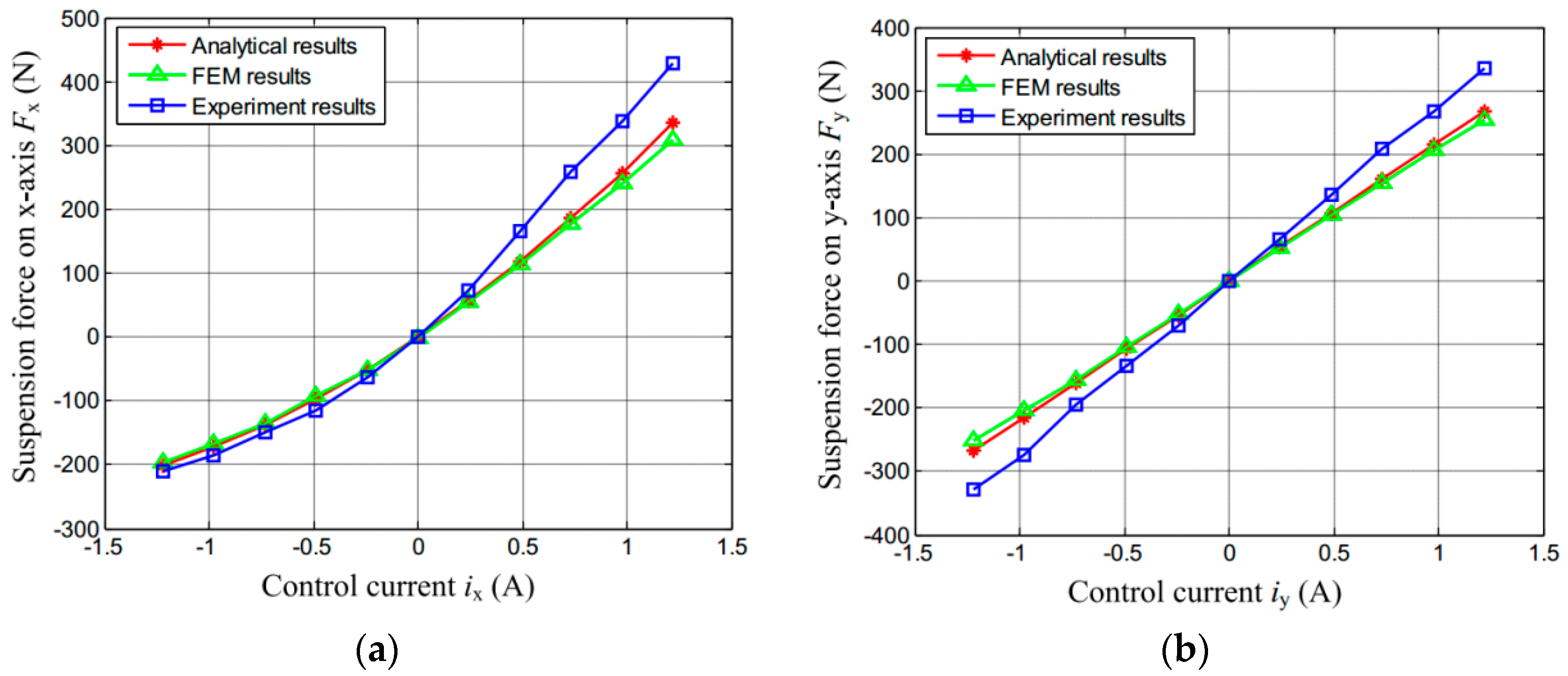
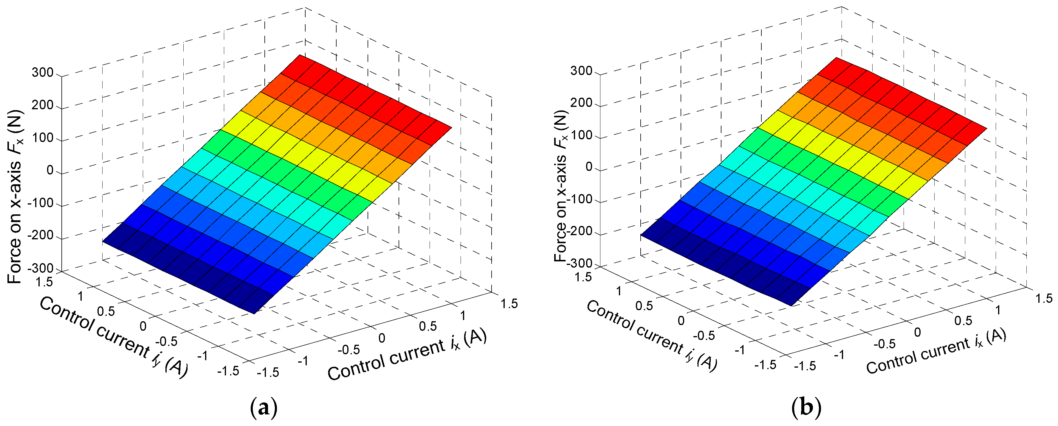
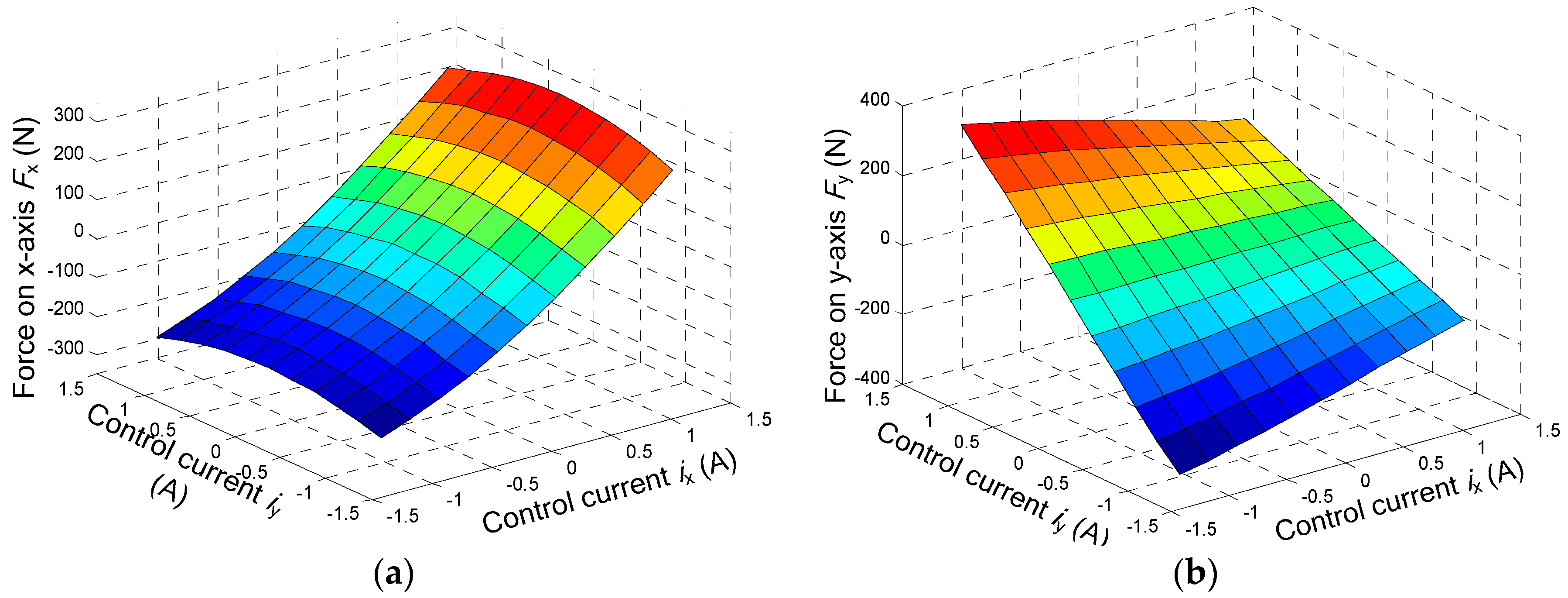
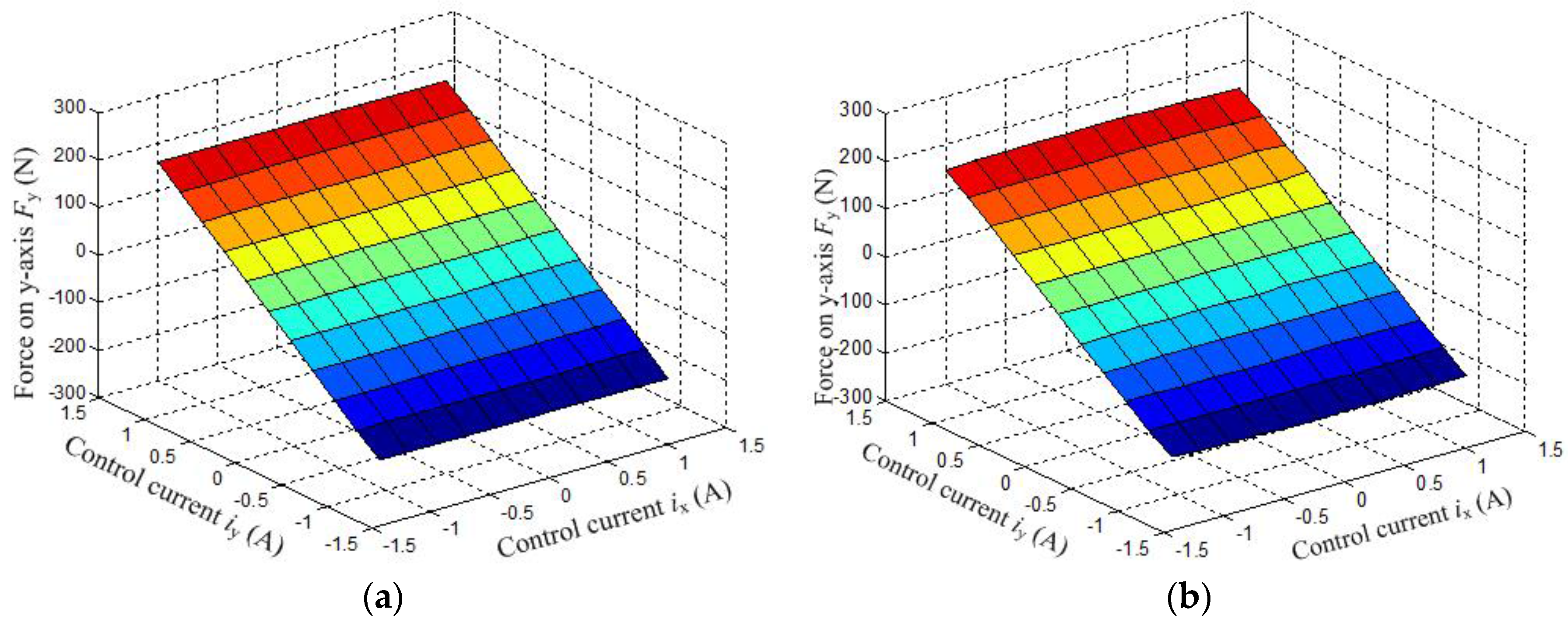
Even when the rotor is in the center position, the relationship between the radial suspension force and radial control current of a three-pole radial-axial HMB is nonlinear. When the current of i_y is constant, the suspension force on the x-axis F_x is a quadratic function of i_x, and the curve of F_x − i_x is a parabola. This characteristic makes the carrying capacity in different directions of coordinate axis different. When i_y is changed, the F_x − i_x curve moves down with the square of i_y. When i_x is constant, the suspension force on the y-axis F_y is linear with i_y, but when i_x is changed, the slope of the F − i_y curve decreases with i_x. As the nonlinearity is obvious, only when the rotor displacement is between [−0.08 mm, 0.08 mm], the three-pole radial-axial HMB can be regarded as a linear system (the air gap length in this paper is 0.5 mm).

(2)

As the magnetic force is a quadratic function of the flux and the flux is linear with control current, the magnetic flux is a quadratic function of the control current, which causes nonlinearity and coupling. However the suspension force on the y-axis is linear with control current. This is because the B-pole and C-pole are symmetric about the x-axis, and the symmetric structure makes the quadratic terms of the B-pole and C-pole offset each other, so it can be deduced that the nonlinearity of the suspension force on the x-axis is caused by both the nonlinear relationship between suspension force and control current and the asymmetric structure of the three radial magnetic poles.

(3)

According to the analysis results, if we add three magnetic poles in the opposite direction of the three radial magnetic poles, the nonlinearity of the radial suspension force and control current can be eliminated. Namely the six-pole radial-axial HMB has better radial suspension force-current performance characteristics. The analytical and FEM results have shown that the relationship between the radial suspension force and control current of a six-pole radial-axial HMB is linear and no coupling exists, so when the rotor displacement is between [−0.2 mm, 0.2 mm], the six-pole radial-axial HMB can be regarded as a linear system (the air gap length in this paper is 0.5 mm).

(4)

The parameters of the three-pole radial-axial HMB and the parameters of the six-pole radial-axial HMB are both designed based on the requirement that the radial carrying capacity is 200 N. It can be calculated that the volume of a six-pole radial-axial HMB is 374,544 mm², which is smaller than the volume of three-pole radial-axial HMB at 549,100 mm², so the six-pole radial-axial HMB has a more compact structure than a three-pole radial-axial HMB with the same radial carrying capacity.

References

1. Schweitzer, G.; Maslen, E.H. Magnetic Bearings: Theory, Design, and Application to Rotating Machinery; Springer-Verlag: New York, NY, USA, 2009. [Google Scholar]
2. Han, B.C.; Zheng, S.Q.; Le, Y.; Xu, S. Modeling and analysis of coupling performance between passive magnetic bearing and hybrid magnetic radial bearing for magnetically suspended flywheel. IEEE Trans. Magn. 2013, 49, 5356–5370. [Google Scholar] [CrossRef]
3. Toh, C.S.; Chen, S.L. Design and control of a ring-type flywheel battery system with hybrid halbach magnetic bearings. In Proceedings of the 2014 IEEE/ASME International Conference on Advanced Intelligent Mechatronics (AIM), Besancon, France, 8–11 July 2014.
4. Hijikata, K.; Takemoto, M.; Ogasawara, S.; Chiba, A.; Fukao, T. Behavior of a novel thrust magnetic bearing with a cylindrical rotor on high speed rotation. IEEE Trans. Magn. 2009, 45, 4617–4620. [Google Scholar] [CrossRef]
5. Noh, M.D.; Cho, S.R.; Kyung, J.H.; Ro, S.; Park, J. Design and implementation of a fault-tolerant magnetic bearing system for turbo-molecular vacuum pump. IEEE/ASME Trans. Machatron. 2005, 10, 626–631. [Google Scholar] [CrossRef]
6. Kim, S.H.; Shin, J.W.; Ishiyama, K. Magnetic bearings and synchronous magnetic axial coupling for the enhancement of the driving performance of magnetic wireless pumps. IEEE Trans. Magn. 2014, 50. [Google Scholar] [CrossRef]
7. Kim, H.Y.; Lee, C.W. Analysis of eddy-current loss for design of small active magnetic bearings with solid core and rotor. IEEE Trans. Magn. 2004, 40, 3293–3301. [Google Scholar] [CrossRef]
8. Bachovchin, K.D.; Hoburg, J.F.; Post, R.F. Stable levitation of a passive magnetic bearing. IEEE Trans. Magn. 2013, 49, 609–617. [Google Scholar] [CrossRef]
9. Fang, J.C.; Wang, C.; Wen, T. Design and optimization of a radial hybrid magnetic bearing with separated poles for magnetically suspended inertially stabilized platform. IEEE Trans. Magn. 2014, 50. [Google Scholar] [CrossRef]
10. Fang, J.C.; Sun, J.J.; Liu, H.; Tang, J. A novel 3-DOF axial hybrid magnetic bearing. IEEE Trans. Magn. 2010, 46, 4034–4045. [Google Scholar]
11. Hou, E.Y.; Liu, K. Investigation of axial carrying capacity of radial hybrid magnetic bearing. IEEE Trans. Magn. 2012, 48, 38–46. [Google Scholar]
12. Imoberdorf, P.; Nussbaumer, T.; Kolar, J.W. Analytical model of current-force characteristics of a combined radial-axial magnetic bearing. In Proceedings of the 12th International Symposium on Magnetic Bearings, Wuhan, China, 21–24 August 2010.
13. Chen, S.L.; Hsu, C.T. Optimal design of a three-pole active magnetic bearing. IEEE Trans. Magn. 2002, 38, 3458–3466. [Google Scholar] [CrossRef]
14. Matsuda, K.; Kanemitsu, Y.; Kijimoto, S. Optimal number of stator poles for compact active radial magnetic bearings. IEEE Trans. Magn. 2007, 43, 3420–3427. [Google Scholar] [CrossRef]
15. Schöb, R.; Redemann, C.; Gempp, T. Radial active magnetic bearing for operation with a 3-phase power converter. In Proceedings of the 4th International Symposium Magnetic Suspension Technology, Gifu, Japan, 30 October–1 November 1997.
16. Hofmann, W. Behaviour and control of an inverter-fed three-pole active radial magnetic bearing. In Proceedings of the 2003 IEEE International Symposium on Industrial Electronics, Janeiro, Brazil, 9–11 June 2003.
17. Beizama, A.M.; Echeverria, J.M.; Martinez-Iturralde, M.; Egaña, I.; Fontan, L. Comparison between pole-placement control and sliding mode control for 3-pole radial magnetic bearings. In Proceedings of the International Symposium on Power Electronics, Electrical Drives, Automation and Motion, Ischia, Italy, 11–13 June 2008.
18. Grbeša, B. Low loss and low cost active radial homopolar magnetic bearing. In Proceedings of the 6th International Symposium on Magnetic Bearings, Cambridge, MA, USA, 5–7 August 1998.
19. Zhang, W.Y.; Zhu, H.Q. Precision modeling method specifically for AC magnetic bearings. IEEE Trans. Magn. 2013, 49, 5543–5553. [Google Scholar] [CrossRef]
20. Zhu, H.Q.; Ling, D.S.; Jv, J.T. Modeling for three-pole radial hybrid magnetic bearing considering edge effect. Energies 2016, 9, 345. [Google Scholar] [CrossRef]
21. Ji, L.; Xu, L.X.; Jin, C.W. Research on a low power consumption six-pole heteropolar hybrid magnetic bearing. IEEE Trans. Magn. 2013, 49, 4918–4926. [Google Scholar] [CrossRef]
22. Xie, Z.Y.; Zhu, H.Q.; Sun, Y.K. Structure and control of AC-DC three-degree-of-freedom hybrid magnetic bearing. In the 8th International Conference on Electrical Machines Systems, Nanjing, China, 27–29 September 2005.
23. Zhu, H.Q.; Ju, J.T. Development of three-pole magnetic bearings and key technologies. Proc. CSEE 2014, 34, 1360–1367. (In Chinese) [Google Scholar]
24. Zhu, H.Q.; Xie, Z.Y.; Zhu, D.H. Principles and parameter design for AC-DC three-degree-of-freedom hybrid magnetic bearings. Chin. J. Mech. Eng. 2006, 19, 534–539. [Google Scholar] [CrossRef]
25. Zhu, H.Q.; Zhang, Z.; Zhu, D.H.; Wang, D.M.; Xie, Z.Y. Structure and finite element analysis of an AC-DC three degrees of freedom hybrid magnetic bearing. Proc. CSEE. 2007, 27, 77–81. (In Chinese) [Google Scholar]
26. Zhang, W.Y.; Zhu, H.Q. Improved model and experiment for AC-DC three-degree-of-freedom hybrid magnetic bearing. IEEE Trans. Magn. 2013, 49, 5554–5565. [Google Scholar] [CrossRef]
27. Zhang, W.Y.; Zhu, H.Q.; Yang, Z.B.; Sun, X.D.; Yuan, Y. Nonlinear model analysis and “switching model” of AC-DC three-degree-of-freedom hybrid magnetic bearing. IEEE/ASME Trans. Mechatron. 2016, 21, 1102–1115. [Google Scholar] [CrossRef]
Figure 1. Structure and flux paths of three-pole radial-axial hybrid magnetic bearings (HMB).
Energies 09 00706 g001
Figure 2. Equivalent magnetic circuit of three-pole radial-axial hybrid magnetic bearings (HMB).
Energies 09 00706 g002
Figure 3. The 3-D finite element method (FEM) model of three-pole radial-axial hybrid magnetic bearings (HMB).
Energies 09 00706 g003
Figure 4. 3-D finite element analysis results of three-pole radial-axial hybrid magnetic bearings (HMB). (a) Force-current characteristics on x-axis; (b) Force-current characteristics on y-axis.
Energies 09 00706 g004
Figure 5. The prototype of three-pole radial-axial hybrid magnetic bearings (HMB).
Energies 09 00706 g005
Figure 6. Suspension force-current characteristics of analytical, finite element method (FEM) and experiment results. (a) Suspension force on x-axis; (b) Suspension force on y-axis.
Energies 09 00706 g006
Figure 7. Structure and flux path of six-pole radial-axial hybrid magnetic bearings (HMB).
Energies 09 00706 g007
Figure 8. The equivalent flux circuit of six-pole radial-axial hybrid magnetic bearings (HMB).
Energies 09 00706 g008
Figure 9. 3-D finite element method (FEM) model of the six-pole radial-axial hybrid magnetic bearings (HMB).
Energies 09 00706 g009
Figure 10. Curves of relationship between suspension force on x-axis and radial control current. (a) Analytical results; (b) Finite element method (FEM) results.
Energies 09 00706 g010
Figure 11. Curves of relationship between suspension force on y-axis and radial control current. (a) Analytical results; (b) Finite element method (FEM) results.
Energies 09 00706 g011