Numerical Modeling and Investigation of Fluid-Driven Fracture Propagation in Reservoirs Based on a Modified Fluid-Mechanically Coupled Model in Two-Dimensional Particle Flow Code

Abstract

Hydraulic fracturing is a useful tool for enhancing rock mass permeability for shale gas development, enhanced geothermal systems, and geological carbon sequestration by the high-pressure injection of a fracturing fluid into tight reservoir rocks. Although significant advances have been made in hydraulic fracturing theory, experiments, and numerical modeling, when it comes to the complexity of geological conditions knowledge is still limited. Mechanisms of fluid injection-induced fracture initiation and propagation should be better understood to take full advantage of hydraulic fracturing. This paper presents the development and application of discrete particle modeling based on two-dimensional particle flow code (PFC^2D). Firstly, it is shown that the modeled value of the breakdown pressure for the hydraulic fracturing process is approximately equal to analytically calculated values under varied in situ stress conditions. Furthermore, a series of simulations for hydraulic fracturing in competent rock was performed to examine the influence of the in situ stress ratio, fluid injection rate, and fluid viscosity on the borehole pressure history, the geometry of hydraulic fractures, and the pore-pressure field, respectively. It was found that the hydraulic fractures in an isotropic medium always propagate parallel to the orientation of the maximum principal stress. When a high fluid injection rate is used, higher breakdown pressure is needed for fracture propagation and complex geometries of fractures can develop. When a low viscosity fluid is used, fluid can more easily penetrate from the borehole into the surrounding rock, which causes a reduction of the effective stress and leads to a lower breakdown pressure. Moreover, the geometry of the fractures is not particularly sensitive to the fluid viscosity in the approximate isotropic model.

1. Introduction

Hydraulic fracturing can be broadly defined as the process by which a fracture is initiated, which subsequently propagates due to hydraulic loading (or hydraulic pressure) applied by a fluid inside the fracture. Examples and applications of hydraulic fracturing can be easily found in geomechanics. Magma-driven dykes can be considered as a natural example, usually in the scale of tens of kilometers [1,2]. Today, fracturing of oil and gas reservoirs, using a mixture of viscous hydraulic fluids and sorted sand, is the most commonly used reservoir stimulation technique [3,4,5]. Other applications of hydraulic fracturing include the disposal of radioactive waste drill cuttings underground [6], heat production from hot dry rock geothermal reservoirs [7,8], as well as the measurement of in situ stresses [9,10,11].

As the geomaterial is opaque, it is impossible to directly observe the subsurface hydraulic-fracture geometries. Thus, properly scaled experimental research and computer numerical simulations based on realistic assumptions are essential to help understand fracture initiation, propagation, intersection, and fracture geometries in geomaterials. The physics of hydraulic fracture complexity are also investigated in laboratory experiments, with the advantage that boundary-conditions are controllable and fracture geometries can be made visible. The drawback of laboratory experiments is the issue of proper scaling to ensure the applicability of results to field operations.

Numerical simulations are another method for analyzing the propagation behavior of hydraulic fractures in naturally fractured reservoirs. In the past few years, great numbers of hydraulic fracturing models have been developed for simulating induced complex fracture networks in subsurface reservoirs [12,13,14,15,16,17,18,19,20,21,22,23]. However, modeling high pressure fluid-driven fracture propagation is still a challenging problem due to the complexity of the stress field around the crack tip conditioned by the geomechanical properties, changing boundary conditions, and complex coupling mechanisms between fluid and solid material. The complexity of the problem often forces researches to consider the rock mass as a homogeneous, isotropic, linear elastic continuum and the fracture geometry as planar, such as in the Khristianovic-Geertsma-de Klerk (KGD) model [14,15] and the Perkins-Kern-Nordgren (PKN) model [12,13]. These assumptions were adapted in some subsequent models [16,17,18,19,20,21,22,23]. Such models are highly simplified and idealized under the assumption of linear elastic fracture mechanism (LEFM), which uses a stress intensity factor at the planar fracture tip as fracture propagation criterion.

Even in the basic form, it is also complicated to mimic hydraulic fracturing process because the model have to take into account the coupling of at least three processes: (1) mechanical deformation induced by the fluid pressure; (2) the flow of fluid within the fracture; and (3) fracture propagation. In recent years, researchers have begun to investigate hydraulic fracture propagation in fractured reservoirs using discontinuum methods, such as the discrete element method (DEM), which originated in the 1970s with two landmark publications on the progressive movement of rock masses as 2-D rigid block assemblages [24,25]. The theoretical foundation of DEM is to formulate and solve the equations of motion of particles or blocks using implicit (based on finite element method discretization) or explicit (using finite volume method discretization) formulations. Usually, the calculated objects is regarded as an assemblage of rigid particles or deformation bodies, which are connected by proper constitute models at their contacts. During the entire motion and deformation process the contacts are continuously updated. Comparing with the continuous methods, the basic character of DEM is that the contact patterns in model are continuously changing with the deformation process. Thus, DEM is a more natural way for modeling fracture initiation, propagation and intersection under complex stress conditions.

Itasca’s universal distinct element code (UDEC) and three-dimensional distinct element code (3DEC) are two representative explicit DEM methods for modeling and assessing complex fracture growth driven by fluids. Choi [26] used UDEC to compare several methods for determining the shut-in pressure during hydraulic fracturing, because owing to the relationship between the behavior of hydraulic fractures and the remote in situ stress, the shut-in pressure is not considered certain. Zangeneh et al. [27] further demonstrated the potential of UDEC for simulating hydraulic fracturing, compared different injection schedules from adjacent wellbores, and their results showed that stress and pore pressure perturbations caused by multiple hydraulic fractures are needed to be considered in the process of wellbore spacing and injection optimization. Zangeneh et al. [28] applied this approach to model fault slip and they were able to use UDEC to estimate the energy release associated with induced seismicity. Zangeneh et al. [29] studied the influence of the orientation of the fracture network relative to that of the ground in situ stress regime with respect to the extent and symmetry of hydraulic fracture propagation. Hamidi and Mortazavi [30,31] used 3DEC for small models to study the hydraulic fracture propagation considering the effects of different fracture fluid rates and fluid properties, tectonic stress regime, and rock mass properties.

A bonded particle model based on particle flow code (PFC) [32] was also used to model hydraulic fracturing [33,34], and the results showed that the model can truly reproduce the physics of injection into low-permeability formations. Through comparisons with results of the geometry of hydraulic fractures from laboratory experiments and field observations of microseismic locations, magnitudes and source mechanisms, Zhao and Young [35] validated the PFC^2D discrete element approach for modeling hydraulic fracturing. Shimizu et al. [36] conducted a series of hydraulic fracturing simulations in competent rock by using flow-mechanically coupled PFC^2D code, and investigated the influence of the fluid viscosity and particle size distribution. Their results show that tensile cracks are dominantly generated in hydraulic fracturing process, while the energy from shear type acoustic emission is larger than tensile type’s. After fracture creation the velocity of fluid infiltrating into the fracture highly depends on the viscosity of the fluid. Eshiet et al. [37] employed PFC^2D to model the pressure development and the subsequent fracturing and/or cavity propagation of bulk rock and sand respectively, considering fluid flow based on the Navier–Stokes equation of an incompressible fluid with contact density. Yoon et al. [38,39,40,41] investigated the fluid injection-induced seismicity in a reservoir for developing an enhanced geothermal system deep underground using discrete element modeling.

UDEC can be used to model progressive failure associated with crack propagation and fault slip by simulating breakage of pre-existing contacts between pre-defined joint bonded deformable but intact blocks. It is also capable of modeling fluid flow through a defined fracture network. Both, UDEC and PFC, can handle coupled hydro-mechanical processes, in which fracture conductivity is dependent on mechanical deformation of joint aperture and, conversely, joint water pressure can affect the mechanical computations of joint aperture. In both models the blocks are treated as impermeable and fracture flow is calculated using a cubic law for joint apertures. Unlike in UDEC, however, where fluid flow is restricted to the fracture flow model, PFC allows not only fluid flow through fractures, but also fluid leak-off into the rock matrix. Furthermore, in the UDEC model, fluid flow into the joint occurs only when a joint is broken, whereas in PFC model fluid flow naturally occurs when a fluid pressure difference exists between neighboring pores. Another difference between the two models is that the blocks in UDEC model are deformable and can generate difference normal stress and normal closure or shear dilation of fractures. Particles are rigid in the PFC model and they can therefore generate different behaviors as in the UDEC model.

It has been validated that the PFC model can simulate fluid flow in rocks, but when it comes to hydraulic fracturing simulations, the fluid-mechanical couple mechanism in PFC still needs to be modified. Our study focuses on investigating hydraulic fracture initiation and propagation by the PFC with modified fluid-mechanical couple mechanism. Firstly, the fluid-mechanical algorithm of the modeling method is introduced and modified. After that, a comparison between the analytical solution of the breakdown pressure and numerically-modeled values is carried out to validate the applicability of the simulation method. Finally, the influence of fluid viscosity, in-situ stress ratio and fluid injection rate on hydraulic fracturing are analyzed using our numerical model, respectively.

2. Modeling Methodology

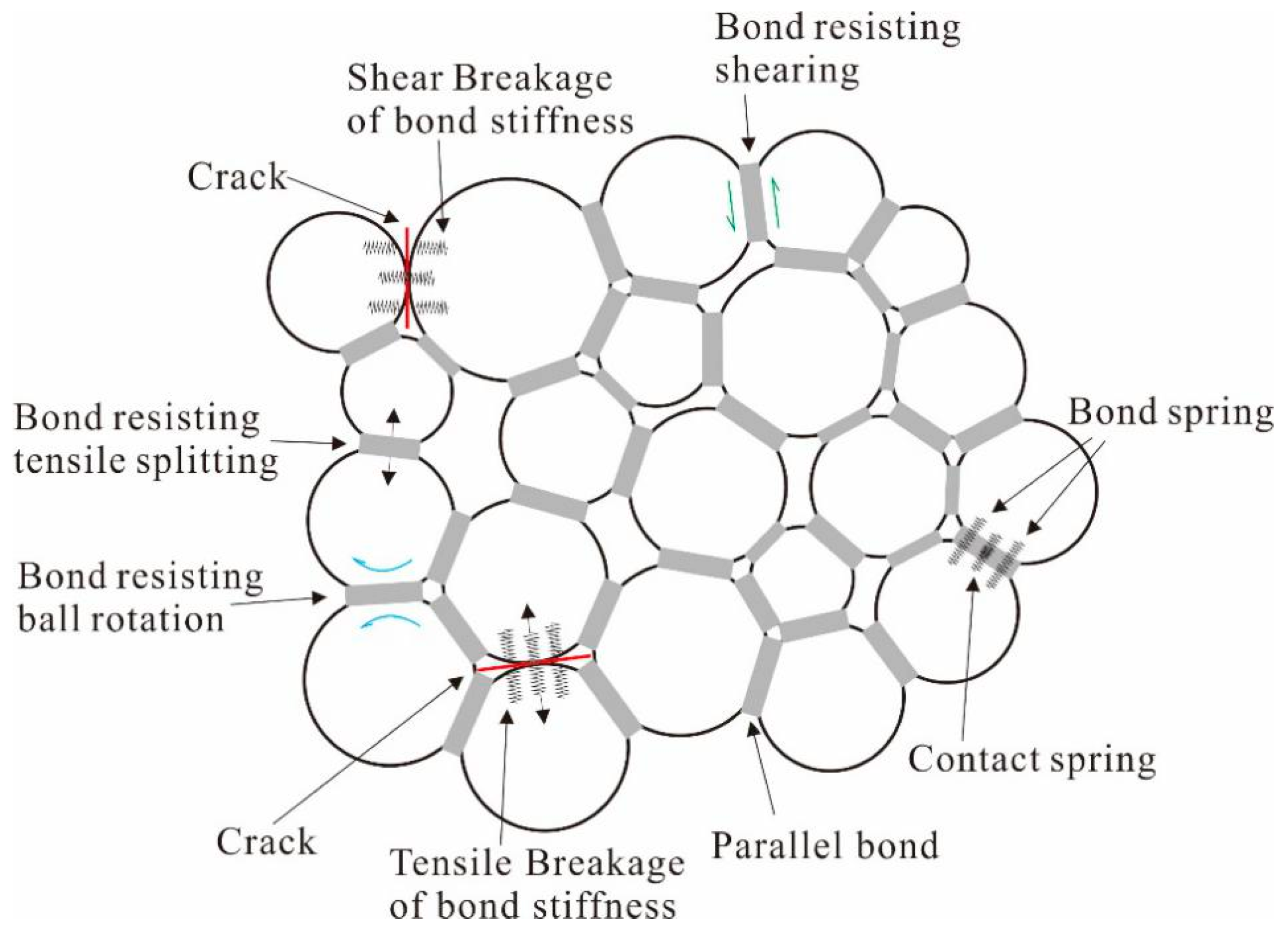
2.1. Particle Flow Code

PFC models the progressive movement and interaction of solid materials represented as bonded circular particles using the DEM, as described by Cundall and Strack [25]. In this study, a two-dimensional distinct element method was employed, and we have modified the code written by Hazzard [33] in order to study fluid-driven fracturing. Since thorough details of the fundamental DEM algorithm can be found in the manuals [32], only a summary of the bonded particle model in PFC^2D code will be given here.

Although the PFC^2D code is a numerical technique that is based on a discontinuum model, it can also be applied to simulate the deformation characteristics of the continuum by introducing bonds between circular particles (Figure 1). The intact rock is simulated as an assemblage of small circular particles. These particles are bonded to their neighbors at the contact points with normal and shear springs and interact with each other. The parallel bond model is commonly used in recent research. In this model, the increments of normal force $\Delta F_i^{\mathrm{n}}$, the tangential force $\Delta F_i^{\mathrm{s}}$ and the moment $\Delta M$ can be calculated from the relative motion of bonded particles, and are given by:

$$\Delta F_i^{\mathrm{n}}=\left(-k^{\mathrm{n}}A\Delta U^{\mathrm{n}}\right){\mathrm{n}}_i$$

(1)

$$\Delta F_i^{\mathrm{s}}=-k^{\mathrm{s}}A\Delta U_i^{\mathrm{s}}$$

(2)

$$\Delta M=-k^{\mathrm{n}}I\Delta \mathsf{\theta } \text{with} \Delta \mathsf{\theta }=\left({\mathsf{\omega }}^{[\mathrm{B}]}-{\mathsf{\omega }}^{[\mathrm{A}]}\right)\Delta t$$

(3)

where kⁿ and k^s are the normal and shear stiffness, respectively; $\Delta U^{\mathrm{n}}$ and $\Delta U_i^{\mathrm{s}}$ are the increments of normal displacement and shear displacement in a timestep, respectively; ${\mathsf{\omega }}^{[\mathrm{A}]}$ and ${\mathsf{\omega }}^{[\mathrm{B}]}$ are the rotation velocities of two bonded particles respectively; n_i is the normal vector of each contact (i = 1 or 2); ∆t is the timestep; A is the cross-sectional area of the bond, and I is the moment of inertia of the bond. The new force and moment associated with parallel bond are calculated by summing the old value existing at the start of the timestep with the increments, and they are given by:

$$F_i^{\mathrm{n}}(t+\Delta t)=F^{\mathrm{n}}(t){\mathrm{n}}_i+\Delta F_i^{\mathrm{n}} \text{with} F^{\mathrm{n}}=F_j^{\mathrm{n}}{\mathrm{n}}_j$$

(4)

$$F_i^{\mathrm{s}}(t+\Delta t)=F_i^{\mathrm{s}}(t)+\Delta F_i^{\mathrm{s}}$$

(5)

$$M(t+\Delta t)=M(t)+\Delta M$$

(6)

The normal stress σ and shear stress τ acting on the cross-section of the bond are calculated by the following equations. The stress is positive when the contact is in compression:

$$\mathsf{\sigma }=\frac{-F^{\mathrm{n}}}{A}+\mathsf{\beta }\frac{\left|M\right|}{I}R$$

(7)

$$\mathsf{\tau }=\frac{\left|F_i^{\mathrm{s}}\right|}{A}$$

(8)

When σ exceeds the normal strength of bond σ_s or τ exceeds the shear strength of bond τ_s, the bonds between the particles can break. The criterions of bond break are summarized as $\left|\mathsf{\sigma }\right|\ge {\mathsf{\sigma }}_{\mathrm{s}} \text{and} \mathsf{\sigma }<0 (\text{Tensile stress})$ and $\left|\mathsf{\tau }\right|\ge {\mathsf{\tau }}_{\mathrm{s}}$, respectively. They imply that the normal bond breaks only by tension, while compression does not cause the bonds to break. If a bond breaks, a micro-crack is generated at the contact point between the particles. The micro-crack length is assumed to be the same as the bond radius R, and the direction of it is perpendicular to the line joining the two centers. The crack is generated automatically under a certain failure criterion with no need for re-meshing.

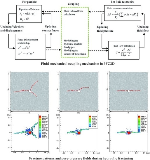
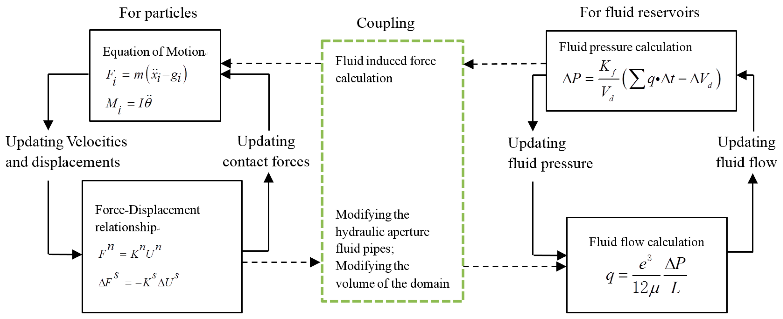
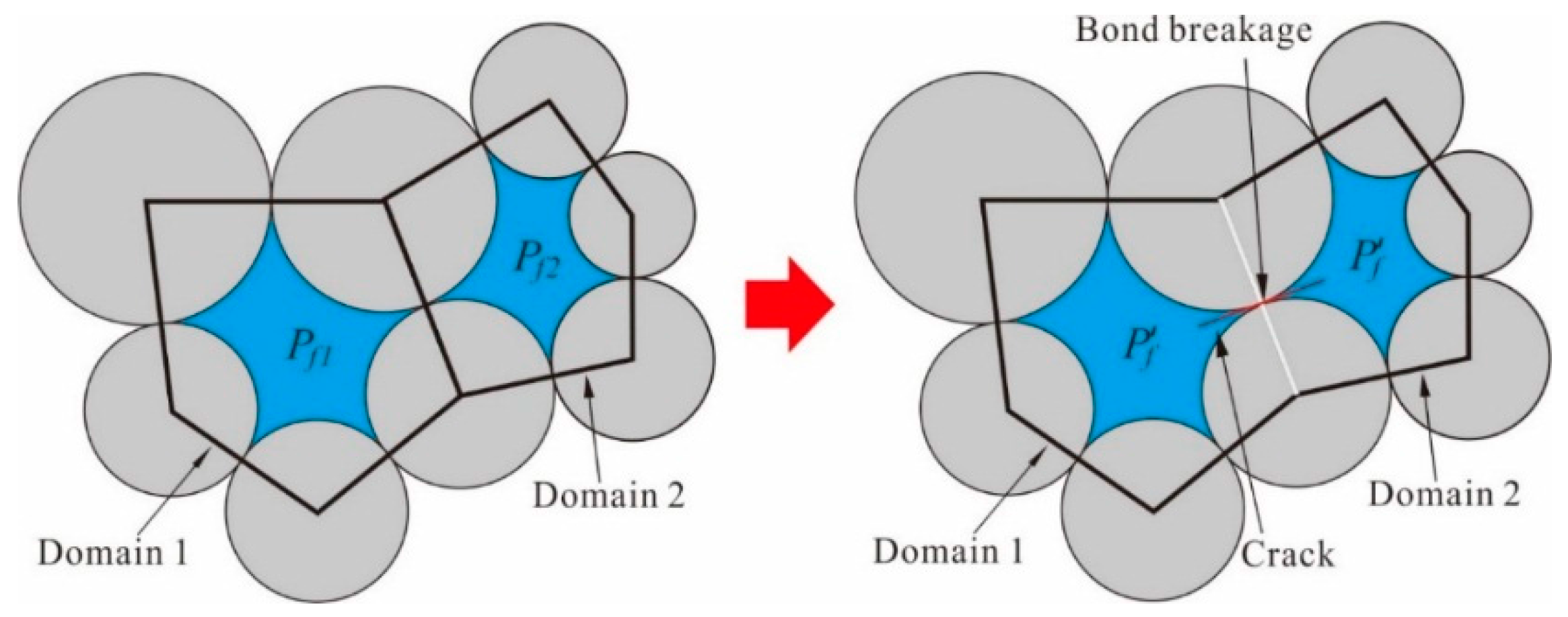
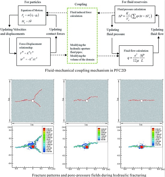
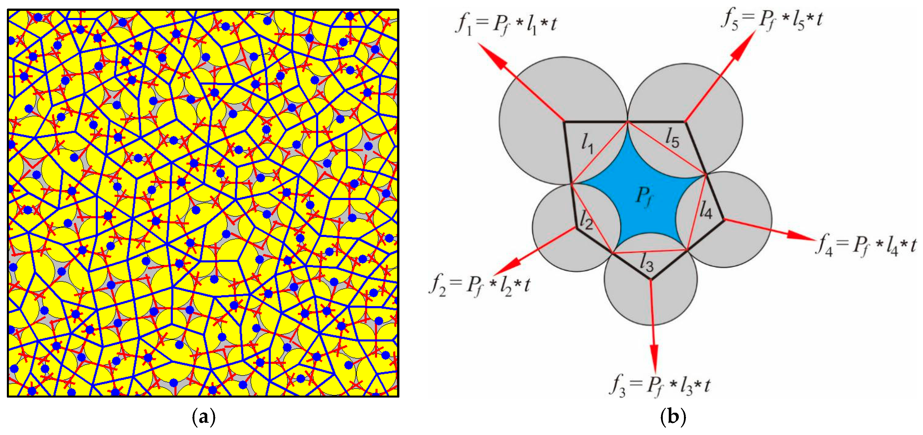
2.2. Fluid-Mechanical Coupling in Two-Dimensional Particle Flow Code

The viscous fluid flow in the bonded particle model is simulated according to the algorithm by Cundall [43], who proposed the original concept of a fluid flow algorithm based on a model that is similar to the network flow model by Thallak et al. [44]. Cundall’s fluid flow algorithm is based on two assumptions; that each particle of the bonded assemblies is a flow channel (pipe), and that these channels connect small reservoirs that store fluid pressure. As shown in Figure 2, the fluid network topology is generated by lines connecting the centers of all particles in contact. The contacts create a series of enclosed domains (Figure 2a, blue polygons), whose centers are stored as a series of reservoirs. The reservoirs are connected by pipes (Figure 2a, red lines), which are perpendicular to corresponding particle contacts. The length of each pipe is calculated as summation of the two particle radii at the contact.. Therefore, each reservoir is completely surrounded by contacts and has a certain volume (void space in an enclosed domain) associated with it.

Flow of viscous fluid in the channel (Figure 2a, red lines) is driven by the differential pressure between the two domains (Figure 2a, blue polygons), and it is modeled using the Poiseuille Equation, assuming that the flow is laminar between two smooth parallel plates. Therefore, the volumetric laminar-flow rate q is given by the following equation:

$$q=\frac{e^3}{12\mathsf{\mu }}\frac{\Delta P}{L}$$

(9)

where e is hydraulic aperture, ∆P is the fluid pressure difference between the two neighboring reservoir domains, L is the length of the flow channel, μ is the fluid dynamic viscosity. The out-of-plane thickness is assumed to be of unit length.

During the fluid flow calculation, the increment of fluid pressure (∆P) in a reservoir is computed from the bulk modulus of fluid (K_f), the volume of the domain (V_d), the sum of the flow volume for one time step (∆t), and the volume change of the domain due to mechanical loading, which is neglected in some studies [33,34], but not in this study. So the equation used is given by:

$$\Delta P=\frac{K_{\mathrm{f}}}{V_{\mathrm{d}}}\left({\displaystyle \sum q\Delta t}-\Delta V_{\mathrm{d}}\right)$$

(10)

Reservoir deformations are caused by the fluid pressure exerted on the surrounding particles (Figure 2b). This force (f) is a product of fluid pressure (P_f), the length (l) exposed to fluid in a domain, and unit thickness (1 m) in out-of-plane direction. The resultant force is then applied to the particles in outward direction normal to the boundary ((Figure 2b), red polygon), which is exposed to fluid.

Figure 3 shows the modeling procedures for a fluid-mechanically coupled system in PFC^2D. In this figure, the simulation of mechanical deformation is shown on the left side, while the simulation of fluid migration is shown on the right size. The deformation of the reservoir causes the increase or decrease of the volume of a domain, also the hydraulic aperture of each flow channel needs to be modified according to the contact force. After the fluid calculation step, fluid pressure in the domain is exerted on the surrounding particles according to Figure 2b.

In the present model, the hydraulic aperture of the flow channel between two particles changes as a function of normal forces. For the particles that are just touching (with 0 effective normal stress) a residual aperture, $e_0$ is assumed. This ensures that fluid can still migrate in a model even without cracks. As the normal force at a contact increases, the aperture related to force can be given as:

$$e=e_{\text{inf}}+(e_0-e_{\text{inf}})\text{exp}(-0.15{\mathsf{\sigma }}_{\mathrm{n}})$$

(11)

where σ_n is the effective normal stress at the contact (in MPa). When σ_n tends to infinity, the aperture decreases asymptotically to $e_{\text{inf}}$. Since flow rate q in Equation (9) is the microscopic flow rate in one flow channel and the fluid flow in a rock model is expressed by an assembly of many flow channels, the permeability of the entire rock model cannot be calculated directly from Equation (9). Therefore, the value of $e_0$ and $e_{\text{inf}}$ are determined according to Equation (12), after Al-Busaidi [34], based on the permeability k of real rock, or by simulating the permeability test corresponding to the characteristics of an actual specimen:

$$k=\frac{1}{12V}{\displaystyle \sum _{\text{pipes}}L{e}^3}$$

(12)

where V is the volume of the reservoir rock, and L is the length of the channel or pipe.

The specimens used in laboratory experiments or field tests are not always saturated. The fluid flow algorithm presented in [33,34] employs the assumption that the entire model is always entirely filled with the fluid. As we know, conditions of variable saturation (dry, saturated, or partially saturated) might have an influence on hydraulic fracturing, due to different fluid pressure, different distribution of microcracks, and different throughout pressure. Therefore, for taking into account the saturation conditions, a saturation factor is introduced in the fluid flow algorithm in this study. The saturation factor in each domain is defined as:

$$S_{\mathrm{t}}=\frac{V_{\mathrm{f}}}{V_{\mathrm{r}}\times \mathsf{\phi }}$$

(13)

where V_r is the volume of domain as shown in Figure 2. V_f is the volume of fluid present in the domain, and $\mathsf{\phi }$ is the porosity of the model. Since the PFC^2D model is an assembly of circular particles, it is difficult to directly considering the porosity of an actual rock accurately. Therefore, the pore volume of the domain is determined by the product of the entire volume of the domain, V_r, and assumed porosity, $\mathsf{\phi }$.

For S_t = 1.0 the domain is saturated, while as S_t < 1.0 the domain is partially saturated. When the partially saturated condition is considered, fluid pressure is assumed to be 0 MPa in this study in the partially saturated domain, and increases only after the domain is saturated. In this study the initial saturation factor S_t is set to 1.0.

When the stresses caused by mechanical force and fluid pressure in each bond exceed the tensile strength or shear strength, a microcrack develops at the contact of neighboring particles. At that time, the hydraulic aperture of the flow pipe related to the bond becomes infinity, which may cause instability in the following calculation. How to simulate the fluid flow in these two domains connected by failed bond plays an important role in hydraulic fracturing in PFC. Hazzard et al. [33], Al-Busaidi et al. [34] and Zhao and Young [35] think that when the bond between two domains fails, the fluid flow is instantaneous, and that the fluid pressure in these domains is assumed to be their average value $P_{\mathrm{f}}^{\prime }$ before the bond failure. The calculation of the new fluid pressure is given as:

$$P_{\mathrm{f}}^{\prime }=\frac{P_{\mathrm{f}1}+P_{\mathrm{f}2}}{2}$$

(14)

where P_f1 and P_f2 are fluid pressure related to Domain 1 and Domain 2, respectively, before the bond failure. However, Equation (13) is not suitable for the condition with a well in the rock model because the volumes of some fluid domains are not approximately equal to each other. Thus, in this study, when the microcrack develops, the fluid pressure of two domains jointed by the failure bond is calculated by Equation (15):

$$P_{\mathrm{f}}^{\prime }=\left[\frac{\left(V_{\mathrm{f}1}+V_{\mathrm{f}2}\right)}{\left(V_{\mathrm{r}1}+V_{\mathrm{r}2}\right) \mathsf{\phi }}-1\right]K_{\mathrm{f}}$$

(15)

where V_f1 and V_f2 are the volume of fluid existing in Domain 1 and Domain 2 in Figure 4, respectively, under 0 MPa fluid pressure, V_r1 and V_r2 are the volume of Domain 1 and Domain 2, respectively.

3. Modeling Validation and Some Scenarios

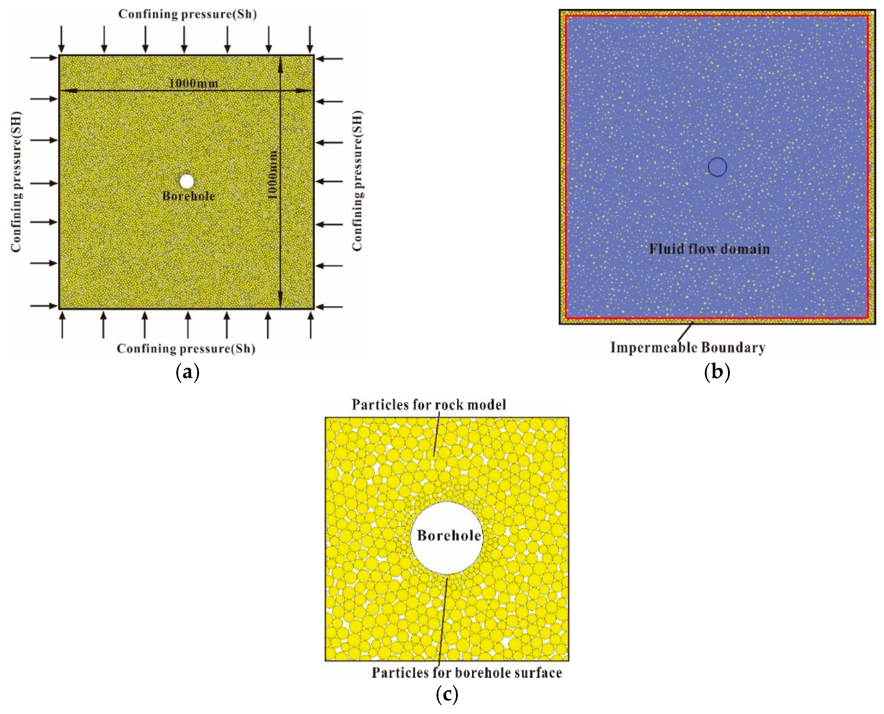
3.1. Model Description and Parameters

Figure 5a illustrates the rock model and loading conditions for hydraulic fracturing. The model is assembled by particles bonded with each other. The size of the rock specimen is 1000 mm in width and 1000 mm in height. The number of circular particles in the model is about 11,700 with particle radii ranging from 4 mm to 6 mm following a normal distribution. A borehole for viscous fluid injection with a diameter of 60 mm is created at the center of the model. The model is surrounded by four walls, which can move to apply the constant confining pressure to the rock model, S_H in the x-direction, and S_h in the y-direction. Figure 5b shows the fluid flow exit domains as a red square. The border of the rock model between the red and black squares is not covered by fluid flow domains and it can be regarded as an impermeable rubber housing. In order to create a smoothed surface within the borehole, the particles surrounding the borehole are substituted by smaller particles with half the mean radius (Figure 5c). The macroscopic and microscopic mechanical parameters used in this study are shown in

Table 1. Rock model properties and input micro-parameters.

Rock Properties	Notations	Values
UCS of rock model (MPa)	σc	46.1
Tensile strength (MPa)	σt	4.4
Young’s modulus (GPa)	E	44.2
Poisson’s ratio	ν	0.20
Porosity (%)	ϕ	10
Permeability (m2)	κ	1 × 10−17
Input micro-parameters	-	-
Lower bound of particle radius (mm)	Rmin	4.0
Ratio of upper bound of particle radius to lower bound of particle radius	Rmin/Rmax	1.5
Particle density (kg/m3)	ρ	3095
Young’s modulus of the particle (GPa)	Ec	32.0
Ratio of normal to shear stiffness of the particle	kn/ks	1.6
Friction coefficient of particle	μ	0.30
Young’s modulus of the parallel bond (GPa)	${\overline{E}}_{\mathrm{c}}$	32.0
Ratio of normal to shear stiffness of the parallel bond	${\overline{k}}_{\mathrm{n}}/{\overline{k}}_{\mathrm{s}}$	1.6
Tensile strength of the parallel bond (MPa)	${\overline{\sigma }}_{\mathrm{t}}$	12.0
Cohesion of the parallel bond (MPa)	$\overline{c}$	30.0
Friction angle of the parallel bond (°)	ϕ	45.0
Radius multiplier	$\overline{\mathsf{\lambda }}$	1.0
Moment contribution factor	β	0.2
Hydraulic Properties	-	-
Initial saturation (%)	St	100
Initial hydraulic aperture (m)	e0 1	2.2 × 10−6
Infinite hydraulic aperture (m)	einf 1	2.2 × 10−7
Bulk modulus of the fracturing fluid (GPa)	Kf	2.0

¹ Calculated according to Equation (12).

.

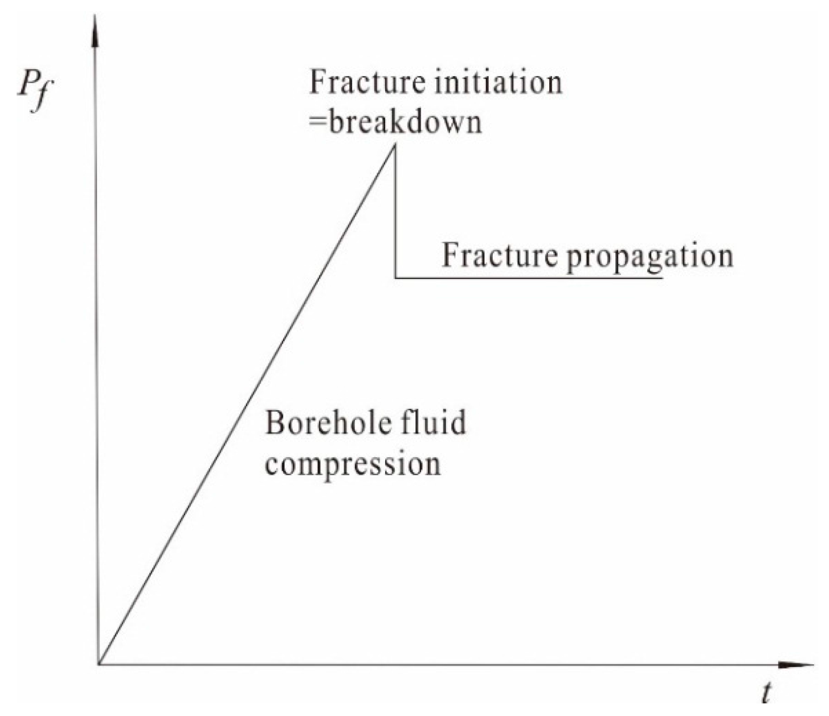
3.2. Validation of Hydraulic Fracturing Model

The possibility of using the bonded particle method to simulate fluid flow in solid materials has been identified by some studies [33,34,35,36,37,38,39,40,45]. However, for modeling hydraulic fracturing not only the fluid flow, but also crack initiation and crack propagation, have to be taken into account. In past research work, the efficiency of the bonded particle method for hydraulic fracturing simulation has been overlooked. In the work of Wang et al. [46] the influence of the initial stress parameters and the tensile strength of a coal seam on the breakdown pressure under certain injection conditions are analyzed, and a regression equation (Equation (10) in Wang et al. [46]) is obtained by fitting curves of hydraulic fracturing simulation results. This regression equation describing stress concentration around a circular elastic borehole is different from the classical Kirsch equations, which have been proposed by Hubbert and Willis [47], Haimson and Fairhurst [48], Fairhurst [49], and Haimson and Cornet [50] as the following expression:

$$P_{\text{wf}}=3S_{\mathrm{h}}-S_{\mathrm{H}}-P_0+{\mathsf{\sigma }}_{\mathrm{t}}$$

(16)

Figure 6 shows the idealized borehole fluid pressure response during hydraulic fracturing. The first linear part reflects the elastic deformation of the fluid and surrounding rock, which is primarily due to compression of the injection fluid in the borehole. The peak represents the crack initial condition, and after this point the fluid pressure drops. This implies a situation of unstable crack development, and the fluid entering the void of cracks. Continued pumping will eventually result in stable crack growth, represented by the constant borehole fluid pressure level. In this idealized case the point of crack initiation and formation breakdown are the same, and the peak corresponds to the breakdown pressure.

In order to validate the reliability of hydraulic fracturing simulation by the bonded particle method, also the influence of the in-situ stress ratio on breakdown pressure is studied under the assumption that the initial pore-pressure is 0 (P₀ = 0), the dynamic viscosity of the injection fluid is 0.001 Pa·s, and the injection rate is fixed at 2.0 × 10⁻⁶ m³/s. Confining pressure in the x-direction (S_H) is set to 20 MPa, and the confining pressure in the y-direction (S_h) changes from 20 MPa to 10 MPa. Figure 7 shows the fluid pressure history at the injection borehole during hydraulic fracturing simulation under different confining pressures in the y-direction. Compared to the idealized fluid pressure history during hydraulic fracturing (Figure 6), the fluid pressure curve in Figure 7 is not linear before arriving at the breakdown pressure. This is because in PFC modeling leakage is taken into account in algorithm design. When fluid is pumped into the borehole, it can according to the cubic law enter the neighbor domains instantaneously through the fluid pipes. Comparing the curves in Figure 7, the conclusion can be arrived at that leakage is increasing with increasing fluid pressure. During unstable growth of hydraulic cracks the fluid pressure also drops. The breakdown pressure values obtained from modeling and the theoretical values calculated according to Equation (16) under different in situ stress ratios are shown in Figure 8. When the ratio of S_H:S_h is between 1.0 and 1.7 the error between the modeled value and the idealized analytical value is less than 20%, where the tensile strength of the rock model is 4.4 MPa. This indicates that hydraulic fracturing simulation by PFC^2D is able to reproduce the realistic processes to an acceptable degree.

3.3. Modeling Scenarios

The performance of hydraulic fracturing is not only related to the mechanical properties of the reservoirs, but also influenced by the in situ stress ratio, the injection flow rate, and the viscosity of the fluid, among others. After the suitability of hydraulic fracturing simulation by bonded particle method was verified in Section 3.2, a comprehensive modeling series of fluid injection into rock mass were performed to investigate the efficiency of hydraulic fracturing at different conditions. In addition to the qualitative evaluation of the modeling results, the model responses, such as injection borehole pressure, crack growth, and fluid pressure variation are compared. In this study, in order to evaluate the effects of confining stresses, the confining boundary conditions are applied to the rock models corresponding to in situ stress ratios of 20:20, 20:15 and 20:12. Previous studies have shown that the fluid injection rate is a key factor to consider [49]. Most operators have found that injection rates should be high to produce a complex crack network. In this work the injection rates of 1.0 × 10⁻⁵, 1.0 × 10⁻⁴ and 5.0 × 10⁻⁴ m³/s are applied in PFC^2D models, respectively. Finally, a dynamic viscosity of the fluid of 1.0 × 10⁻², 1.0 × 10⁻³ and 1.0 × 10⁻⁴ Pa·s are also simulated, respectively.

4. Modeling Results and Discussion

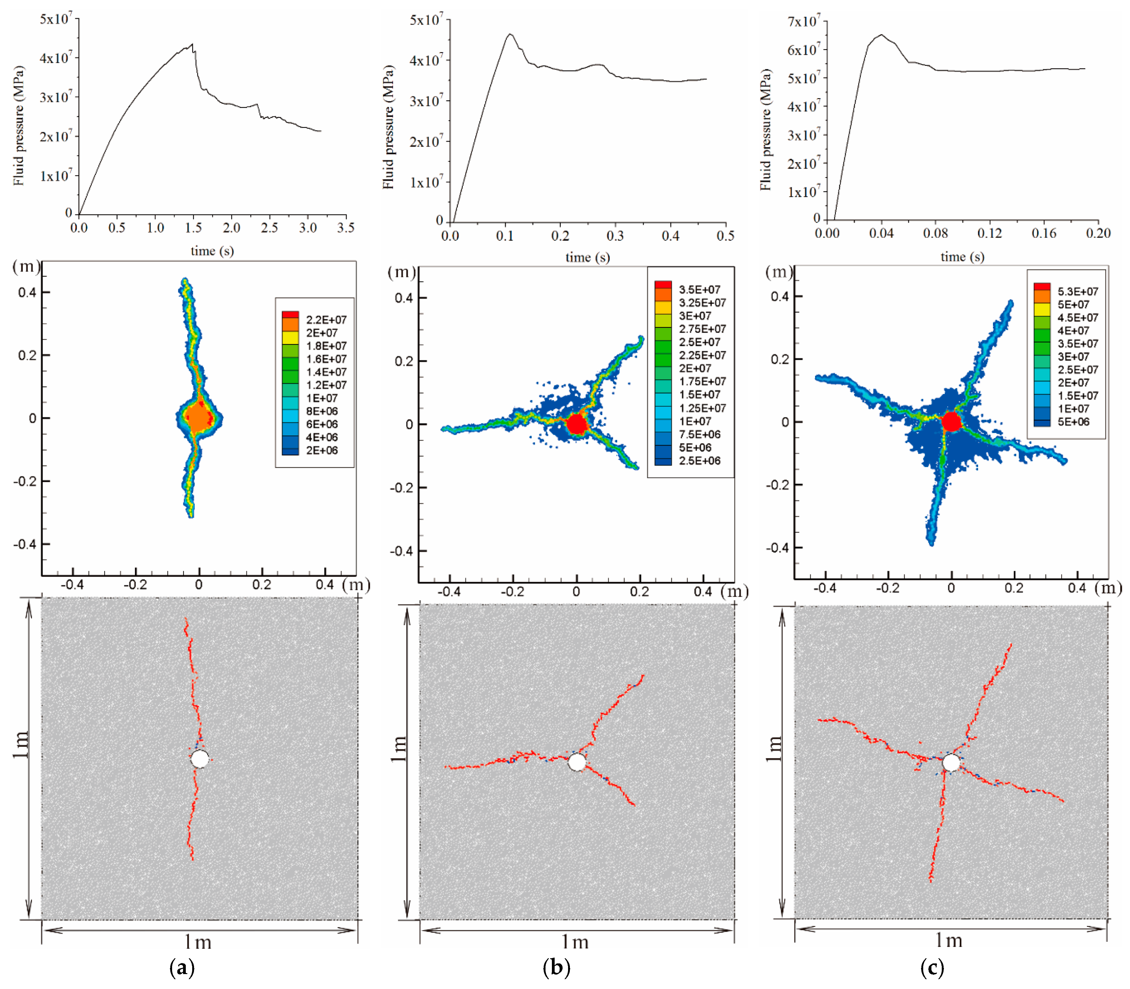
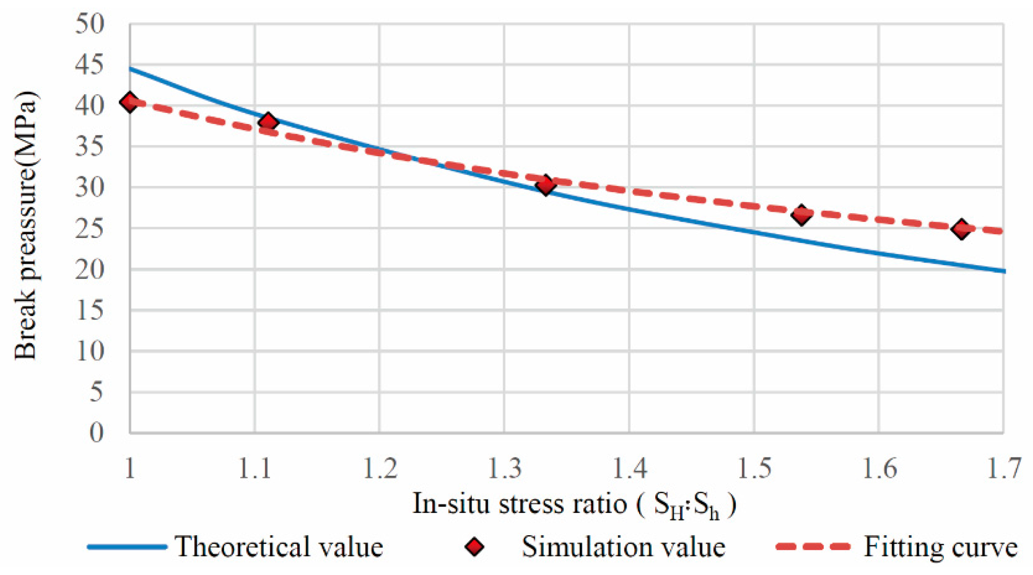
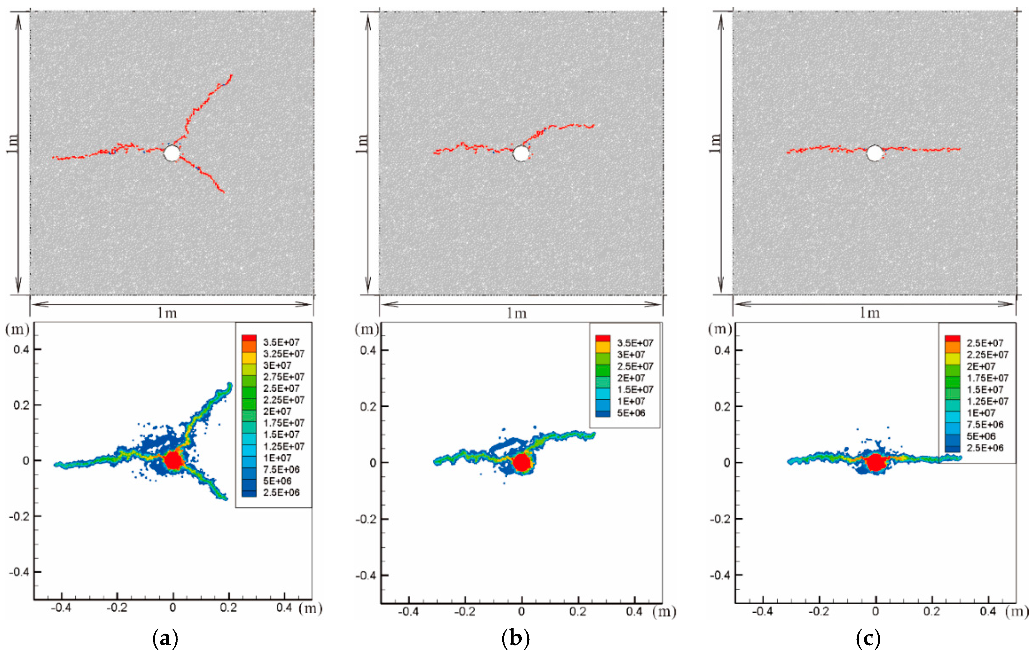
4.1. The Influence of in Situ Stress

Although the influence of confining pressure on fluid breakdown pressure has already been discussed in Section 3.2, in this section the influence of the in-situ stress on hydraulic crack development, as well as fluid pressure surrounding the borehole and cracks is investigated in a general situation, where the viscosity of the fluid is 1.0 × 10⁻³ Pa·s, while the micro-mechanical parameters and initial permeability in the rock models remain unchanged. The stress in the x-direction (S_H) is always 20 MPa, while the stress in the y-direction (S_h) is varied between 12, 15 and 20 MPa, respectively. Under the assumption that the hydraulic apertures of fluid flow pipes conform to Equation (11), the average initial apertures in these models are 5.33 × 10⁻⁷, 4.98 × 10⁻⁷ and 4.55 × 10⁻⁷ m, respectively. With increasing fluid pressure in the domains, the aperture can reach 1.03 × 10⁻⁶ m when the bonding stress condition between particles is tension.

Figure 9 shows the borehole pressure variation with injection time and crack distributions with the corresponding fluid pressure at three different time steps during the hydraulic fracturing process under the injection rate of 1.0 × 10⁻⁵ m³/s. According to the borehole pressure histories corresponding to those described above, the time of fluid injection before the borehole pressure drops firstly increases with increasing S_h, and the breakdown pressures are 27.1, 33.5 and 43.5 MPa, respectively. In our numerical results, most of micro-fractures were tensile fractures, which developed when the tensile stress exceeded the tensile strength between the bonded circular particles. Generally, the major hydraulic fracture initiated in a preferred direction which is affected by the in-situ stress and model formation. As described by Hubbert and Willis [47], the crack propagation direction is controlled by the in situ stress ratio. At the same time, the micro anisotropy of PFC models, especially the defects in surrounding rock of injection borehole, is the other factor for hydraulic fracture initiation.

As presented in Figure 9a,b, when S_H:S_h = 20:12 and S_H:S_h = 20:15, the major fractures stated at the borehole surface in the direction of maximum principle stress (horizontal direction), which can be attributed to the tensile stress concentration at these locations. While S_H:S_h = 20:20, tensile stress concentration is not distinct because the model is in a hydraulic pressure condition. Thus, the defect in the borehole surface of the PFC model is the main factor for fracture initiation and propagation in vertical direction in Figure 9c. The crack patterns at different times show that hydraulic crack propagation is not symmetric and simultaneously in this study, and it can be divided into two steps. Firstly, the failure takes place at the weakest bond surrounding the injection borehole, and cracks propagate along a direction with borehole pressure drop. Then, after the crack extended to a certain length, the bond failure at the other side of the borehole is initiated. These processes are different from the results of Zhang et al. [11], where the cracks developed symmetrically.

When assuming that the fluid injection rate was 1.0 × 10⁻⁴ m³/s, Figure 10 shows that when S_H:S_h = 20:20, there are three main fractures developing in three different directions, while with S_H:S_h = 20:15, there are only two main fractures, which initially extend deviating from the direction of maximum principle stress and then along it. When S_H:S_h = 20:12, two main fractures extend along the direction of maximum principle stress right from the beginning. As previous research shows [47], the direction of maximum principle stress is a kind of preferred direction for fracture initiation and propagation during deep hydraulic fracturing. Figure 10b is a typical example, where the combination of maximum principle stress direction and modeled defects control the fracture pattern. Due to the defects at the borehole surface, the major fracture initiated in a non-preferred direction, while it turned and twisted during propagation and tended to be aligned with the preferred direction. Comparing the fracture patterns in Figure 9 and Figure 10, the conclusion can be arrived at that injection rate is a key factor in hydraulic fracturing, which will be further analyzed in the following section.

The fluid pressure in the borehole and the available space can drive crack growth; at the same time, the pore-pressure changes due to cracks development and the deformation of the reservoir. Figure 9 and Figure 10 both show that the distribution of fractures is corresponding with the pore pressure field.

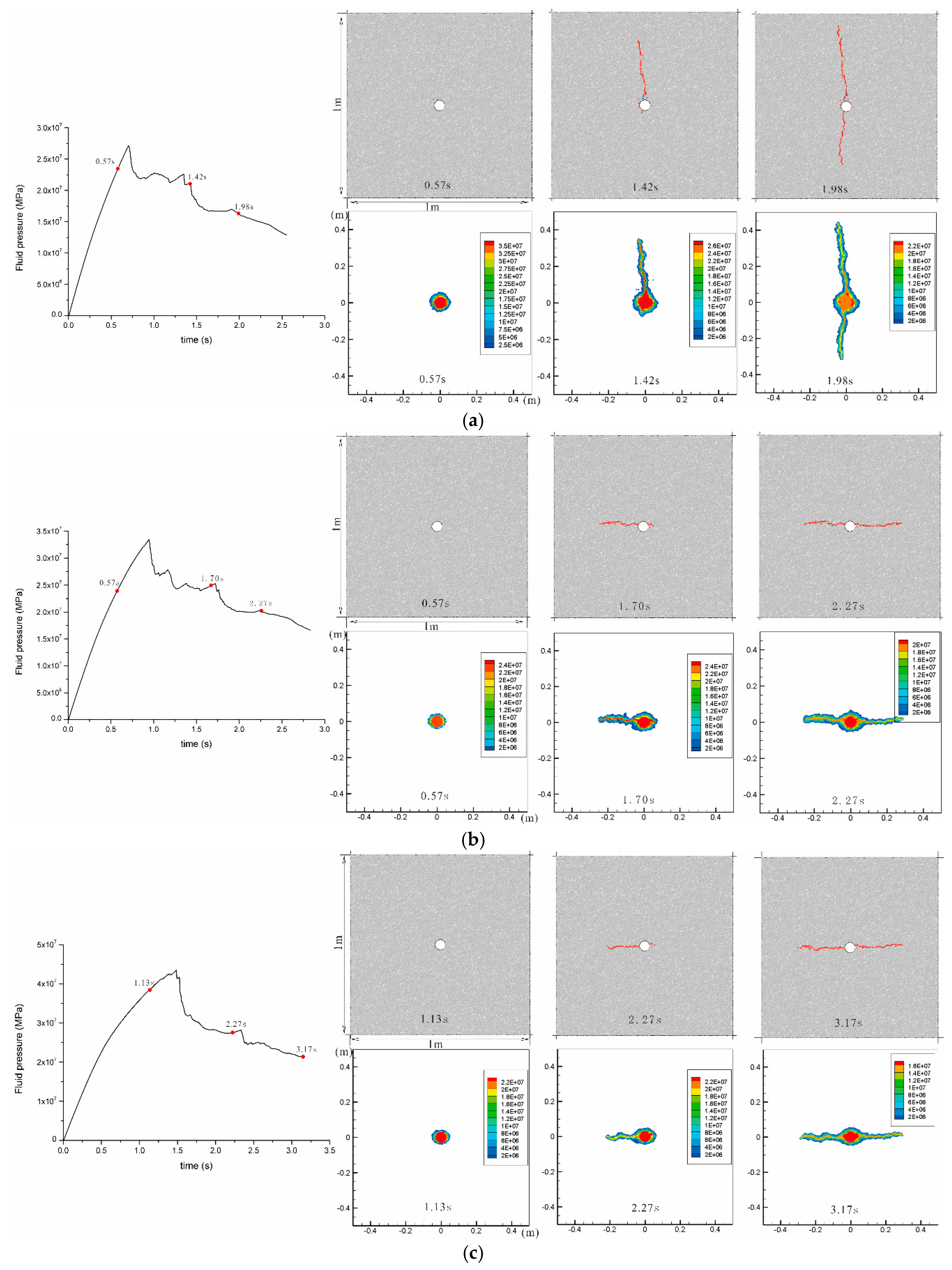
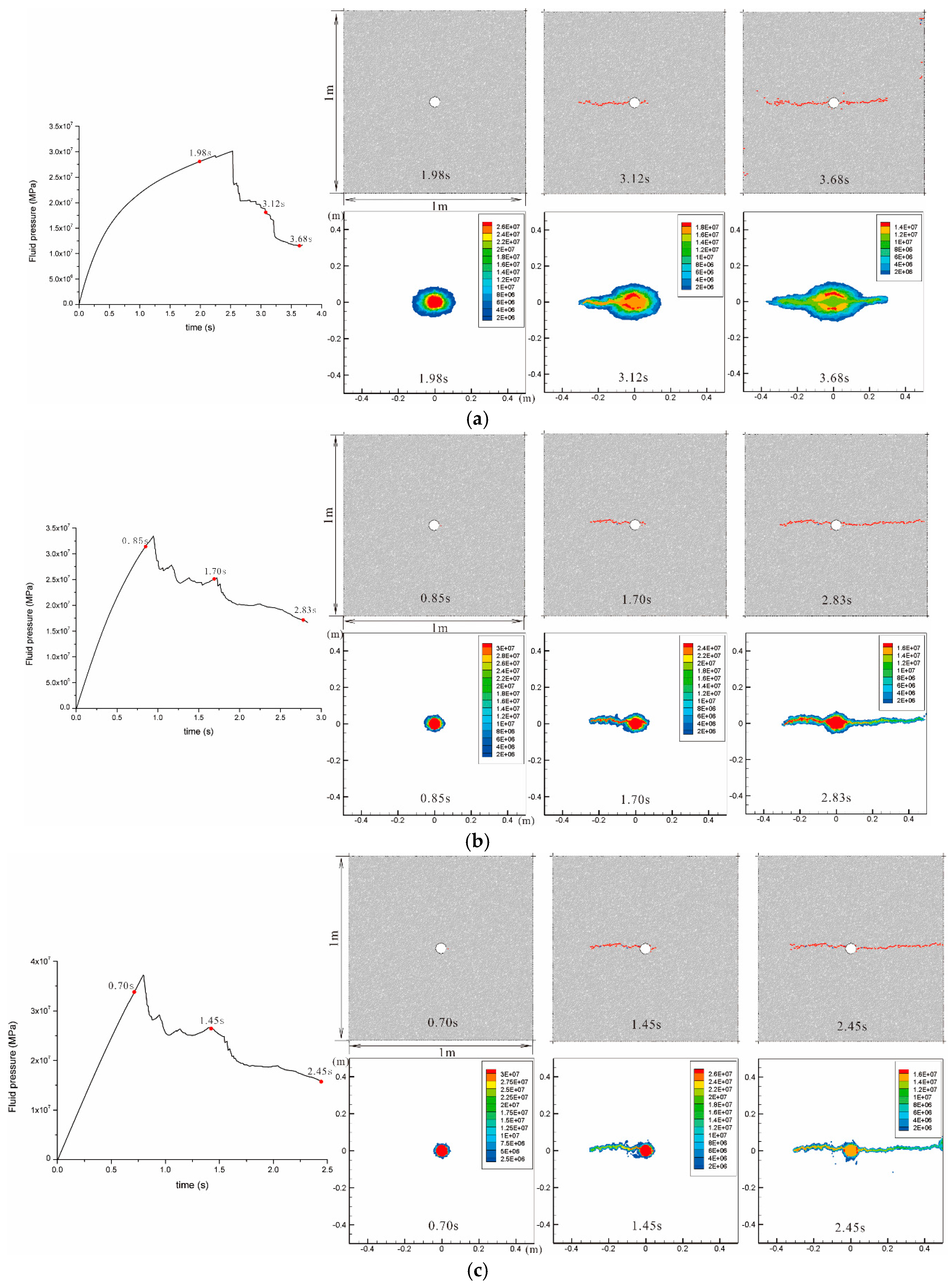
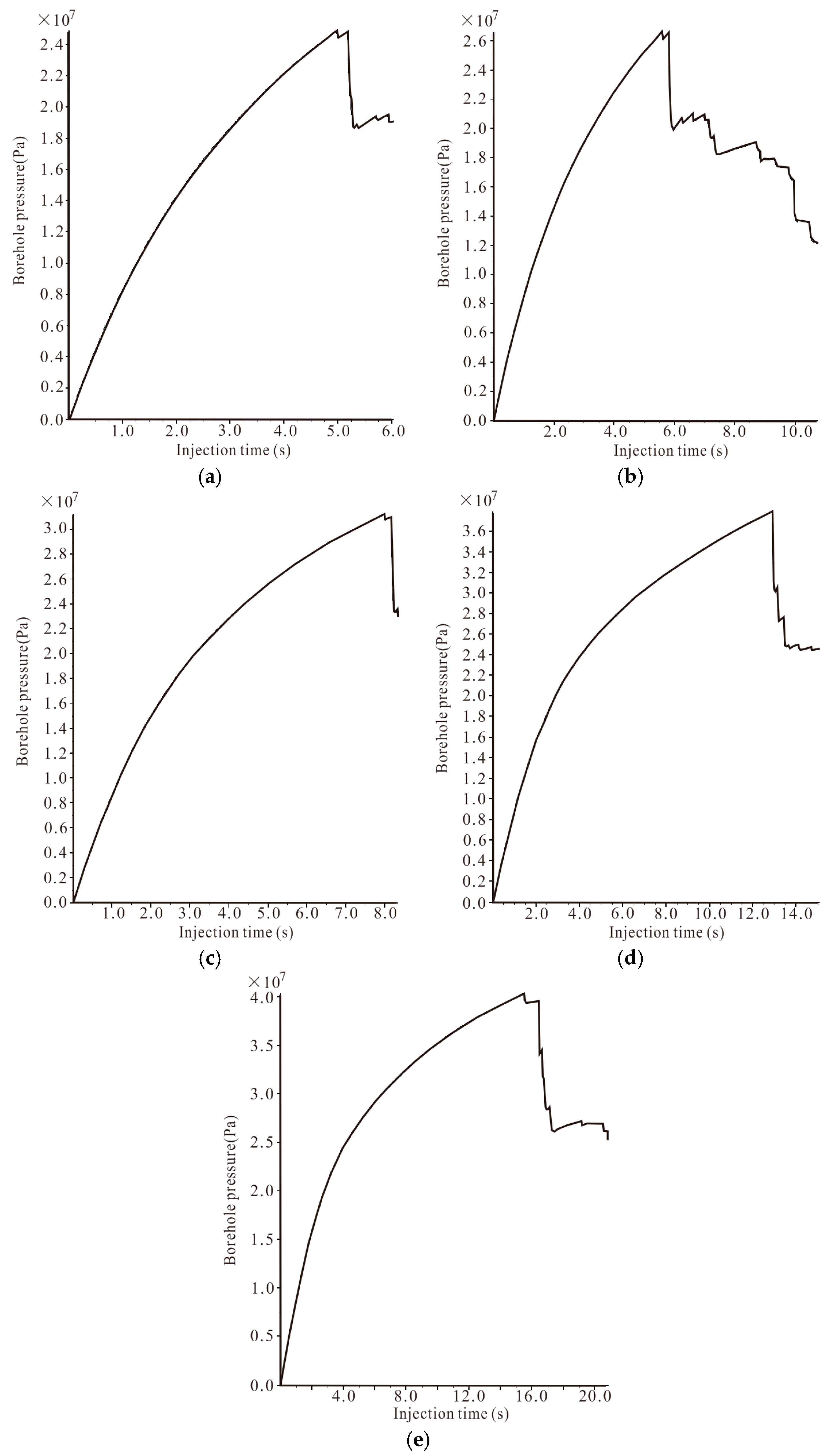
4.2. The Influence of the Rate of Fluid Injection

From the previous studies, fluid injection rate plays an important role in hydraulic fracturing [10]. Most operators have found that injection rates should be high to accomplish complex crack networks. In this section, the influence of injection rate on hydraulic fracturing characteristics were investigated. The viscosity of fluid is 1.0 × 10⁻³ Pa·s, and the confining pressure in both the x-direction and the y-direction are 20 MPa. Three injection rates are applied in modeling, which are 1.0 × 10⁻⁵, 1.0 × 10⁻⁴ and 5.0 × 10⁻⁴ m³/s, respectively.

The modeling results are shown in Figure 11. The borehole pressure histories show that the breakdown pressures are 43.6, 46.5 and 65.3 MPa, respectively, under these three injection rates. The breakdown pressure increases as the injection rate increases, and also the injection time before the fluid pressure dropping decreases. When the injection rate is high, the stress in the solid skeleton caused by the borehole pressure has not adjusted, which leads to a higher breakdown pressure. This process is consistent with observations from rock uniaxial tests in the laboratory. In Figure 11, the pore-pressure field in models shows that the pore pressure increase caused by reservoir skeleton deformation is more pronounced as the injection rate increases, which can also be an effect of the local stress concentration around the injection borehole. Additionally, Figure 11 shows two main fractures that developed when the injection rate was 1.0 × 10⁻⁵ m³/s, while four main fractures grew under the injection rate of 5.0 × 10⁻⁴ m³/s. Thus, more main fractures could generate under higher injection rates, which is consistent with observations made in previous researches.

4.3. The Influence of Fluid Viscosity

Ishida et al. [51] carried out hydraulic fracturing experiment using injection fluid of different viscosities in laboratory and their study shows that the viscosity of the fracturing fluid has an influence on the mechanism of crack generation, crack initial pressure and breakdown pressure. Chen et al. [52] also investigated how the viscosity of the fracturing fluid affects fracture propagation using three different viscosities (viscous oil, water, and supercritical CO₂), and the results show that hydraulic fracturing with low viscosity fluids form a more complex fracture network in rocks. In this section the effect of the viscosity of the fracturing fluid on crack initiation and propagation are discussed, which were simulated under conditions with an injection rate of 1.0 × 10⁻⁵ m³/s, and a confining pressure of 20 MPa in the x-direction and 15 MPa in the y-direction. The results are shown in Figure 12 for three different fluid viscosities of 1.0 × 10⁻⁴, 1.0 × 10⁻³ and 1.0 × 10⁻² Pa·s, respectively. The corresponding breakdown pressures are 31.2, 33.4 and 37.2 MPa, respectively. At the lowest fluid viscosity, the crack initiation and propagation pressure was lower than at higher fluid viscosities.

This result is attributed to pore pressure gradient around the borehole induced by fluid infiltration. As the borehole pressure increases, fracturing fluid penetrates into the interconnected pores from the borehole wall, which causes an increased pore pressure around the borehole. The pore pressure reduces the effective stress of the rock near the borehole, which facilitates the generation of cracks. Figure 12 also shows that with the low viscosity fluid the volume filled by fluid with pore-pressure P_f > 1.0 MPa is larger. This shows that the low viscosity fluid can more easily infiltrate the rock. After cracks evolved, the fracturing fluid penetrates into the void instantaneously, which causes the borehole pressure to drop. The borehole pressure can be lower than the pore pressure in the surrounding rock (Figure 12a). So, if the borehole pressure drops sharply due to the fracture extending, the pore pressure in rock is much higher than the fluid pressure in borehole, which can easily cause the failure of the rock surrounding the borehole.

5. Conclusions

A series of simulations for hydraulic fracturing in rock was performed by using a modified fluid, mechanically coupled model in PFC^2D, to investigate the influence of the in situ stress states, the fracturing fluid injection rate, and the fluid viscosity on the geometries of hydraulic fractures and pore-pressure field, respectively. The modeling results show good agreement with previous laboratory works, and the main results are summarized as following:

(1)

In this study, in all cases, except for the model under hydrostatic stress state (the confining pressures are equal both in x-direction and y-direction), the orientation of hydraulic fractures is parallel to the direction of maximum compressive principle stress. This result verifies that the influence of in situ stress was appropriately expressed in the PFC^2D simulation.

(2)

Different injection rates in hydraulic fracturing represent different loading scenarios. Similar to in-rock dynamic testing, high injection rates correspond to a larger strain rate loading way. Thus, the breakdown pressure increases as the injection rate increases. When the injection rate is high, the stress in the solid skeleton caused by the borehole pressure cannot adjust instantaneously and local stress concentrations prevail, which leads to a higher breakdown pressure. In this case, complex geometry of fractures can be formed with a predomination of micro-cracks.

(3)

Breakdown pressure with the low viscosity fluid was lower than with high viscosity fluid. Fracturing fluid can more easily penetrate through the interconnected domains into the rock from the borehole wall, and so the pore pressure increases around the borehole, which causes the effective stress reduction. Finally, the breakdown pressure with the low viscosity fluid was lower than that with high viscosity fluid. The geometry of the fractures is found to be not very sensitive to the fluid viscosity.

As we know, in laboratory hydraulic fracturing experiments or actual hydraulic fracturing operations, it is difficult to directly observe the crack initiation and propagation and changes of stress and fluid pressure distribution due to the fluid injection. In this study, PFC^2D was successfully applied to study the hydraulic fracturing process. This demonstrates that the bonded particle method is a useful and strong tool for understanding the fracturing behavior of reservoir rocks. The hydraulic fracturing of naturally fractured reservoirs will be studied in following research by PFC^2D.

References

1. Rubin, A.M. Propagation of magma-filled cracks. Ann. Rev. Earth Planet. Sci. 1995, 23, 287–336. [Google Scholar] [CrossRef]
2. Spence, D.A.; Turcotte, D.L. Magma-driven propagation of cracks. J. Geophys. Res. Solid Earth 1985, 90, 575–580. [Google Scholar] [CrossRef]
3. Adachi, J.; Siebrits, E.; Peirce, A.; Desroches, J. Computer simulation of hydraulic fractures. Int. J. Rock Mech. Min. Sci. 2007, 44, 739–757. [Google Scholar] [CrossRef]
4. Vermylen, J.; Zoback, M.D. Hydraulic fracturing, microseismic magnitudes, and stress evolution in the Barnett Shale, Texas, USA. In Proceedings of the SPE Hydraulic Fracturing Technology Conference, The Woodlands, TX, USA, 24–26 January 2011.
5. Fisher, K.; Warpinski, N. Hydraulic fracture height growth: Real data. SPE Prod. Oper. 2012, 27, 8–19. [Google Scholar] [CrossRef]
6. De Laguna, W.; Tamura, T.; Weeren, H.O.; Struxness, E.G.; McClain, W.C.; Sexton, R.C. Engineering Development of Hydraulic Fracturing as a Method for Permanent Disposal of Radioactive Wastes; Oak Ridge National Lab.: Oak Ridge, TN, USA, 1968. [Google Scholar]
7. Zimmermann, G.; Tischner, T.; Legarth, B.; Huenges, E. Pressure-dependent production efficiency of an enhanced geothermal system (EGS): Stimulation results and implications for hydraulic fracture treatments. Pure Appl. Geophys. 2009, 166, 1089–1106. [Google Scholar] [CrossRef]
8. Zimmermann, G.; Moeck, I.; Blöcher, G. Cyclic waterfrac stimulation to develop an enhanced geothermal system (EGS)—Conceptual design and experimental results. Geothermics 2010, 39, 59–69. [Google Scholar] [CrossRef]
9. Yokoyama, T.; Sano, O.; Hirata, A.; Ogawa, K.; Nakayama, Y.; Ishida, T.; Mizuta, Y. Development of borehole-jack fracturing technique for in situ stress measurement. Int. J. Rock Mech. Min. Sci. 2014, 67, 9–19. [Google Scholar] [CrossRef]
10. King, G.E. Thirty years of gas shale fracturing: What have we learned? In Proceedings of the SPE Annual Technical Conference and Exhibition, Florence, Italy, 19–22 September 2010.
11. Zhang, B.; Li, X.; Zhang, Z.; Wu, Y.; Wu, Y.; Wang, Y. Numerical investigation of influence of in-situ stress ratio, injection rate and fluid viscosity on hydraulic fracture propagation using a distinct element approach. Energies 2016, 9, 140. [Google Scholar] [CrossRef]
12. Perkins, T.K.; Kern, L.R. Widths of hydraulic fractures. J. Pet. Technol. 1961, 13, 937–949. [Google Scholar] [CrossRef]
13. Nordgren, R.P. Propagation of a vertical hydraulic fracture. Soc. Pet. Eng. J. 1972, 12, 306–314. [Google Scholar] [CrossRef]
14. Khristianovic, S.; Zheltov, Y. Formation of vertical fractures by means of highly viscous fluids. In Proceedings of the 4th World Petroleum Congress, Rome, Italy, 6–15 June 1955; Volume 2, pp. 579–586.
15. Geertsma, J.; De Klerk, F. A rapid method of predicting width and extent of hydraulically induced fractures. J. Pet. Technol. 1969, 21, 1571–1581. [Google Scholar] [CrossRef]
16. Cleary, M.P. Comprehensive design formulae for hydraulic fracturing. In Proceedings of the SPE Annual Technical Conference and Exhibition, Dallas, TX, USA, 21–24 September 1980.
17. Barree, R.D. A practical numerical simulator for three-dimensional fracture propagation in heterogeneous media. In Proceedings of the SPE Reservoir Simulation Symposium, San Francisco, CA, USA, 15–18 November 1983.
18. Shaffer, R.J.; Thorpe, R.K.; Heuze, F.E.; Ingraffea, A.R. Numerical and physical studies of fluid-driven fracture propagation in jointed rock. In Proceedings of the 25th US Symposium on Rock Mechanics (USRMS), Pittsburgh, PA, USA, 13–15 May 1984.
19. Ventura, J.L. Slator Ranch fracture optimization study. J. Pet. Technol. 1985, 37, 1251–1262. [Google Scholar] [CrossRef]
20. Meyer, B.R. Three-dimensional hydraulic fracturing simulation on personal computers: Theory and comparison studies. In Proceedings of the SPE Eastern Regional Meeting, Morgantown, WV, USA, 24–27 October 1989.
21. Mohaghegh, S.; Balanb, B.; Platon, V.; Ameri, S. Hydraulic fracture design and optimization of gas storage wells. J. Pet. Sci. Eng. 1999, 23, 161–171. [Google Scholar] [CrossRef]
22. Dong, C.Y.; De Pater, C.J. Numerical modeling of crack reorientation and link-up. Adv. Eng. Softw. 2002, 33, 577–587. [Google Scholar] [CrossRef]
23. Reynolds, M.; Shaw, J.; Pollock, B. Hydraulic fracture design optimization for deep foothills gas wells. J. Can. Pet. Technol. 2004, 43. [Google Scholar] [CrossRef]
24. Cundall, P.A. A computer model for simulating progressive, large-scale movements in blocky rock systems. In Proceedings of the International Symposium on Rock Fracture, Nancy, France, 4–6 October 1971.
25. Cundall, P.A.; Strack, O.D.L. A discrete numerical model for granular assemblies. Geotechnique 1979, 29, 47–65. [Google Scholar] [CrossRef]
26. Choi, S.O. Interpretation of shut-in pressure in hydrofracturing pressure-time records using numerical modeling. Int. J. Rock Mech. Min. Sci. 2012, 50, 29–37. [Google Scholar] [CrossRef]
27. Zangeneh, N.; Eberhardt, E.; Bustin, R.M. Investigation of the influence of stress shadows on multiple hydraulic fractures from adjacent horizontal wells using the distinct element method. In Proceedings of the 21st Canadian Rock Mechanics Symposium, RockEng 2012-Rock Engineering for Natural Resources, Edmonton, AB, Canada, 5–9 May 2012; pp. 445–454.
28. Zangeneh, N.; Eberhardt, E.; Bustin, R.M.; Bustin, A. A numerical investigation of fault slip triggered by hydraulic fracturing. In Proceedings of the ISRM International Conference for Effective and Sustainable Hydraulic Fracturing, Brisbane, Australia, 20–22 May 2013.
29. Zangeneh, N.; Eberhardt, E.; Bustin, R.M. Investigation of the influence of natural fractures and in situ stress on hydraulic fracture propagation using a distinct-element approach. Can. Geotech. J. 2015, 52, 926–946. [Google Scholar] [CrossRef]
30. Hamidi, F.; Mortazavi, A. Three dimensional modeling of hydraulic fracturing process in oil reservoirs. In Proceedings of the 46th US Rock Mechanics/Geomechanics Symposium, Chicago, IL, USA, 24–27 June 2012.
31. Hamidi, F.; Mortazavi, A. A new three dimensional approach to numerically model hydraulic fracturing process. J. Pet. Sci. Eng. 2014, 124, 451–467. [Google Scholar] [CrossRef]
32. PFC2D—Particle Flow Code in 2 Dimensions; Version 4.0; Itasca Consulting Group Inc.: Minneapolis, MN, USA, 2008.
33. Hazzard, J.F.; Young, R.P.; Oates, S.J. Numerical modeling of seismicity induced by fluid injection in a fractured reservoir. In Proceedings of the 5th North American Rock Mechanics Symposium Mining and Tunnel Innovation and Opportunity, Toronto, ON, Canada, 7–10 July 2002; pp. 1023–1030.
34. Al-Busaidi, A.; Hazzard, J.F.; Young, R.P. Distinct element modeling of hydraulically fractured Lac du Bonnet granite. J. Geophys. Res. Solid Earth 2005, 110. [Google Scholar] [CrossRef]
35. Zhao, X.; Young, P.R. Numerical modeling of seismicity induced by fluid injection in naturally fractured reservoirs. Geophysics 2011, 76, WC167–WC180. [Google Scholar] [CrossRef]
36. Shimizu, H.; Murata, S.; Ishida, T. The distinct element analysis for hydraulic fracturing in hard rock considering fluid viscosity and particle size distribution. Int. J. Rock Mech. Min. Sci. 2011, 48, 712–727. [Google Scholar] [CrossRef]
37. Eshiet, K.I.; Sheng, Y.; Ye, J. Microscopic modelling of the hydraulic fracturing process. Environ. Earth Sci. 2013, 68, 1169–1186. [Google Scholar] [CrossRef]
38. Yoon, J.S.; Zang, A.; Stephansson, O. Numerical investigation on optimized stimulation of intact and naturally fractured deep geothermal reservoirs using hydro-mechanical coupled discrete particles joints model. Geothermics 2014, 52, 165–184. [Google Scholar] [CrossRef]
39. Yoon, J.S.; Zimmermann, G.; Zang, A. Numerical investigation on stress shadowing in fluid injection-induced fracture propagation in naturally fractured geothermal reservoirs. Rock Mech. Rock Eng. 2015, 48, 1439–1454. [Google Scholar] [CrossRef]
40. Yoon, J.S.; Zimmermann, G.; Zang, A. Discrete element modeling of cyclic rate fluid injection at multiple locations in naturally fractured reservoirs. Int. J. Rock Mech. Min. Sci. 2015, 74, 15–23. [Google Scholar] [CrossRef]
41. Yoon, J.S.; Zimmermann, G.; Zang, A.; Stephansson, O. Discrete element modeling of fluid injection—Induced seismicity and activation of nearby fault 1. Can. Geotech. J. 2015, 52, 1457–1465. [Google Scholar]
42. Cho, N.; Martin, C.D.; Sego, D.C. A clumped particle model for rock. Int. J. Rock Mech. Min. Sci. 2007, 44, 997–1010. [Google Scholar] [CrossRef]
43. Cundall, P. Fluid Formulation for PFC2D; Itasca Consulting Group: Minneapolis, MN, USA, 2000. [Google Scholar]
44. Thallak, S.; Rothenburg, L.; Dusseault, M. Simulation of multiple hydraulic fractures in a discrete element system. In Proceedings of the 32nd US Symposium on Rock Mechanics (USRMS), Norman, OK, USA, 10–12 July 1991.
45. Chang, M.; Huang, R.C. Observations of hydraulic fracturing in soils through field testing and numerical simulations. Can. Geotech. J. 2016, 53, 343–359. [Google Scholar] [CrossRef]
46. Wang, T.; Zhou, W.; Chen, J.; Xiao, X.; Li, Y.; Zhao, X. Simulation of hydraulic fracturing using particle flow method and application in a coal mine. Int. J. Coal Geol. 2014, 121, 1–13. [Google Scholar] [CrossRef]
47. Hubbert, M.K.; Willis, D.G. Mechanics of hydraulic fracturing. Petr. Trans. AIME. 1957, 210, 153–168. [Google Scholar]
48. Haimson, B.; Fairhurst, C. Initiation and extension of hydraulic fractures in rocks. Soc. Pet. Eng. J. 1967, 7, 310–318. [Google Scholar] [CrossRef]
49. Fairhurst, C. Stress estimation in rock: A brief history and review. Int. J. Rock Mech. Min. Sci. 2003, 40, 957–973. [Google Scholar] [CrossRef]
50. Haimson, B.C.; Cornet, F.H. ISRM suggested methods for rock stress estimation—Part 3: Hydraulic fracturing (HF) and/or hydraulic testing of pre-existing fractures (HTPF). Int. J. Rock Mech. Min. Sci. 2003, 40, 1011–1020. [Google Scholar] [CrossRef]
51. Ishida, T.; Chen, Q.; Mizuta, Y.; Roegiers, J.-C. Influence of fluid viscosity on the hydraulic fracturing mechanism. J. Energy Resour. Technol. 2004, 126, 190–200. [Google Scholar] [CrossRef]
52. Chen, Y.; Nagaya, Y.; Ishida, T. Observations of fractures induced by hydraulic fracturing in anisotropic granite. Rock Mech. Rock Eng. 2015, 48, 1455–1461. [Google Scholar] [CrossRef]
Figure 1. Illustration of the parallel bond model (modified from Cho [42]).
Energies 09 00699 g001
Figure 2. Particle flow code model used in the fluid-mechanical simulation: (a) fluid network (yellow circles are solid particles; domains (blue polygons), the centers of domains (blue circles), and flow channels (red lines) making up the fluid network); and (b) mechanical coupling. Red arrows are resultant forces applied to the particles surrounding the domain due to the fluid pressure Pf.
Energies 09 00699 g002
Figure 3. Modeling procedures for a fluid-mechanical coupling.
Energies 09 00699 g003
Figure 4. Bond breakage and fluid pressure balancing according to Equation (15) in two related domains.
Energies 09 00699 g004
Figure 5. Rock specimen model and loading conditions: (a) rock specimen model and loading condition; (b) fluid flow domain and impermeable boundary; and (c) particle packing method near borehole.
Energies 09 00699 g005
Figure 6. Idealized borehole fluid pressure response during hydraulic fracturing.
Energies 09 00699 g006
Figure 7. Fluid pressure history at injection borehole during hydraulic fracturing simulation under different confining pressure in y-direction: (a) Sh = 12.0 MPa; (b) Sh = 13.0 MPa; (c) Sh = 15.0 MPa; (d) Sh = 18.0 MPa; and (e) Sh = 20.0 MPa.
Energies 09 00699 g007
Figure 8. Breakdown pressures obtained from modeling and theoretical calculation based on Equation (16) at different in situ stress ratio (SH:Sh).
Energies 09 00699 g008
Figure 9. Borehole pressure histories and crack distribution with corresponding pore-pressure field in hydraulic fracturing with an injection rate of 1.0 × 10⁻⁵ m3/s under different in situ stress ratios: (a) SH:Sh = 20:12; (b) SH:Sh = 20:15; and (c) SH:Sh = 20:20.
Energies 09 00699 g009
Figure 10. Crack distribution with corresponding pore-pressure field under the injection rate of 1.0 × 10⁻⁴ m3/s: (a) SH:Sh = 20:20; (b) SH:Sh = 20:15; and (c) SH:Sh = 20:12.
Energies 09 00699 g010
Figure 11. Borehole pressure histories and crack distribution with corresponding fluid pressure in hydraulic fracturing with a fluid viscosity of 1.0 × 10⁻³ Pa·s under different injection rates: (a) 1.0 × 10⁻⁵ m3/s; (b) 1.0 × 10⁻⁴ m3/s; and (c) 5.0 × 10⁻⁴ m3/s.
Energies 09 00699 g011
Figure 12. Borehole pressure histories and crack distribution with corresponding fluid pressure states in hydraulic fracturing with the injection rate of 1.0 × 10⁻⁵ m3/s and three different fluid viscosities: (a) 1.0 × 10⁻⁴ Pa·s; (b) 1.0 × 10⁻³ Pa·s; and (c) 1.0 × 10⁻² Pa·s.
Energies 09 00699 g012