Article

A Proposal on Low Frequency AC Transmission as a Multi-Terminal Transmission System

by
Achara Pichetjamroen
* and
Toshifumi Ise
Graduate School of Engineering, Osaka University, 2-1 Yamada-oka, Suita, Osaka 565-0871, Japan
*
Author to whom correspondence should be addressed.
Energies 2016, 9(9), 687; https://doi.org/10.3390/en9090687
Submission received: 27 June 2016 / Revised: 5 August 2016 / Accepted: 18 August 2016 / Published: 29 August 2016

Abstract

:
This paper is focused on the discussion and comparison of characteristics and behavior of three low frequency ac (LFAC) transmission system configurations operating under the same control scheme and conditions to identify the most promising operation system for LFAC. Merits of LFAC over high voltage direct current (HVDC) are mentioned first. By changing power flow direction without auxiliary switches in multi-terminal application and easiness of short circuit protection are explained. The three configurations of LFACs are described and applied by the control scheme with the aid of the tool of the PSCAD/EMTDC software to consider the behavior of each LFAC system on line frequency and low frequency sides. For two-phase system, no fluctuation occurs on the line frequency side, which is the advantage over single-phase system. Furthermore, current rating on thyristor devices during operation and number of devices that used in each type of LFAC are calculated and compared. These results can lead to determine the most suitable transmission system for the LFAC system operation.

1. Introduction

High Voltage Direct Current (HVDC) is widely applied for point to point connection between power systems. Since HVDC cable transmission is not affected by the capacitance, HVDC systems are feasible for long transmission line lengths. However, when increasing the interconnection using HVDC for off-shore wind turbines, multi-terminal HVDC (MTDC) is utilized. Currently two basic converter technologies, conventional Line-Commutated Current Source Converters (LCC) and self-commutated Voltage Source Converters (VSCs) including Modular Multi-level Converter (MMC), are mostly used in the HVDC systems.
LCC-HVDC still remains the dominant technology for long distance bulk power transmission due to its lower investment costs and much higher maximum power transfer capacities. It is naturally able to withstand short circuit currents due to the fact the DC inductors limit the current during fault conditions. Power reversal in MTDC however usually needs a complicated switching technique in the case LCCs are used [1].
On the other hand, VSC-HVDC systems are sensitive to DC line faults. When a faults occurs on the DC side of a VSC-HVDC system, an insulated-gate bipolar transistor IGBT cannot control it and the freewheeling diodes work as a bridge rectifier, so it is not able to withstand large surge currents, and may be damaged before the fault is cleared. Some solutions are proposed, however additional control and the switching devices are needed.
Besides LCC-HVDC and VSC-HVDC, high-voltage low-frequency ac transmission system (LFAC) has been proposed as a promising transmission system that can be a compromise between the advantages and disadvantages of both transmission systems. The LFAC transmission system can reduce capacitive currents, and offer simplicity for over-current protection.
In general, the main advantage of the LFAC technology is to significantly reduce power losses due to decreased transmitting frequency. The increase of power capacity and transmission distance compared to the conventional (50 or 60 Hz) transmission ac system can be mentioned as its main advantages [2]. Protection of low frequency side faults is easier than for the DC side faults of VSC-HVDC due to their zero crossing point; also the power flow direction can be changed by the phase control of the voltage on the low frequency side [3], and existing circuit breakers can be used in this system although the interruption current is decreased to around half of 60 Hz [4].
LFAC transmission has been studied for wind power applications due to the increasing number of interconnections between new wind power installations and the grid [5,6]. The capability of handling large amounts of power as more generation is injected as multi-terminal system is a positive feature of the system.
Although some studies on LFAC control schemes were carried out [7,8], previous investigations have not considered the various types of LFAC system configurations that could be operated in the system. Three LFAC system configurations, namely single-phase, two-phase, three-phase are studied. The rest of paper is organized as follows: the merits of the LFAC system are shown in Section 2. Three configurations are described in Section 3. The control scheme is outlined in Section 4. In Section 5, a simulation study with a comparison between each system is provided and the comparison of current ratings on the devices, number of transmission lines and current rating among the three types of LFAC are shown to evaluate the most suitable configuration for LFAC operation. Finally, conclusions are given in Section 6.

2. Merits of Low-Frequency AC Transmission System LFAC

The merits of the LFAC system are explained in the following subsections.

2.1. Multi-Terminal Application

In case of LCC-MTDC, as shown in Figure 1, the LCC-HVDC configuration using current source converter has an obvious problem to operate in this system. Mechanical switches are necessary to change the voltage polarity to reverse the power flow direction at terminal C.
The VSC-HVDC transmission system shown in Figure 2 can change the direction of its power flow without reversing the polarity of the current of DC cables, which is suitable for multi-terminal systems. However, the fault protection for during short-circuits on DC line is considered a drawback of this system compared to the LCC-MTDC system.
Besides the two types of multi-terminal HVDC, the multi-terminal LFAC (LCC-MTLF) as shown in Figure 3 is an alternative transmission system. It can solve all these problems by designing a controller that can synchronize the firing angle of cycloconverters in each terminal following a transmitting power reference in appropriate directions.

2.2. Short Circuit Current

In the case of the LFAC transmission system shown in Figure 3, operation by an LCC converter type has the natural ability to withstand short circuits as the DC inductors can assist in limiting the currents during fault operating conditions. Moreover, when a fault occurs on a low frequency line, it does not need to shut down the whole system due to the existence of inductance on low frequency lines so that the LFAC transmission system can continue to operate partially by disconnecting the faulted line.

2.3. Synchronization

When the number of VSC converter stations increases in an HVDC transmission system, the complexity of the master control increases. The coordinated control needs the information for proper coordination between terminals to share the amount of transmitting power to each terminal. To set active power sharing, a fast telecommunication link is needed for the synchronization of the converter orders as shown in Figure 4.
To avoid this control complexity, the LCC-MTLF can be employed by applying the power synchronization control which make each terminal has a dynamic response similar to a synchronous machine which is virtual synchronous generator (VSG) [3,9]. The concept of control scheme is shown in Figure 5.

3. Configuration

The three configurations of the LFAC transmission systems are studied in this section.

3.1. Single-Phase System

The single-phase system consists of two sets of 12-pulse cycloconverters connected via cable. This configuration can be operated by using zero phase difference between upper and lower parts.
Figure 6 shows the single-phase configuration of low frequency ac transmission system. Each side consists of three phase (Y-∆) and (Y-Y) transformers, and two sets of 12-pulse AC-AC converter are connected to the power cable. At sending end, the cycloconverter works as frequency converter changing from utility ac input voltage from 60 Hz to low frequency during transmitting power. At receiving end, another cycloconverters works as frequency converter by changing low frequency to 60 Hz of ac voltage. By operating LFAC with single-phase system, the fluctuation problem occurs on the line frequency side, because the in-phase operation on single-phase cannot avoid this problem as show in Figure 7. For this reason, a two-phase system is introduced in next section.

3.2. Two-Phase System

Similar to the proposed circuit configuration from a single-phase system, the same configuration can be also used for a two-phase system with 90° phase differences between each phase. Figure 8 shows that this configuration also uses a two-phase system for the low frequency ac transmission system. There are two single-phase sets with 12-pulse cycloconverters, the upper part called α-phase and the lower part called β-phase, with the same rating and topology, so the total amount of transmitted power can be equally shared in each phase. To operate this system configuration, a 90° phase difference between them is required. This operation can maintain constant power on the frequency side, which is one of the merits of this configuration.
Power fluctuation analysis can be done using Figure 8. The power equation from the low frequency side can be stated as follows:
P α = ( V L F sin θ ) ( I L F sin θ ) P β = ( V L F sin ( θ π 2 ) ) ( I L F sin ( θ π 2 ) ) P a c = P α + P β     = ( V L F sin θ ) ( I L F sin θ ) + ( V L F sin ( θ π 2 ) ) ( I L F sin ( θ π 2 ) ) ; θ = 0 °     =   V L F I L F
The calculated fluctuation power on line frequency side P a c from (1) can be confirmed considering the 90° of phase difference between two-phase operations of the LFAC transmission system. The total power from the line frequency side is constant.

3.3. Three-Phase System

Figure 9 shows a three-phase low frequency ac transmission system configuration. This system has a similar configuration as the previous two-phase transmission system. In this configuration one more phase is added compared with the two-phase configuration. This three-phase system configuration can be described as including phase a, phase b and phase c. Each phase has a 120° phase difference among them. The advantage on this configuration is that it keeps the instantaneous power constant on the line frequency side.

4. Control Scheme

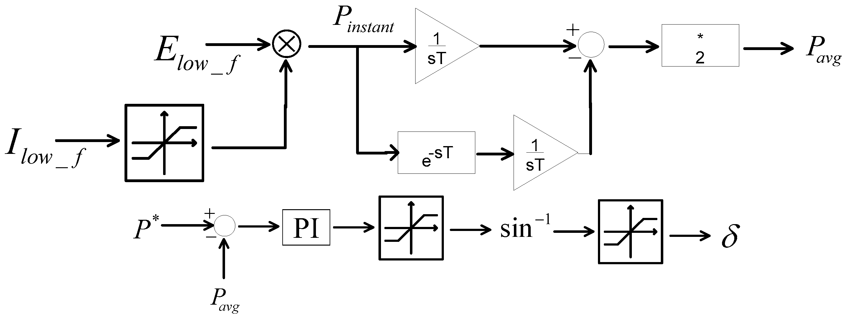
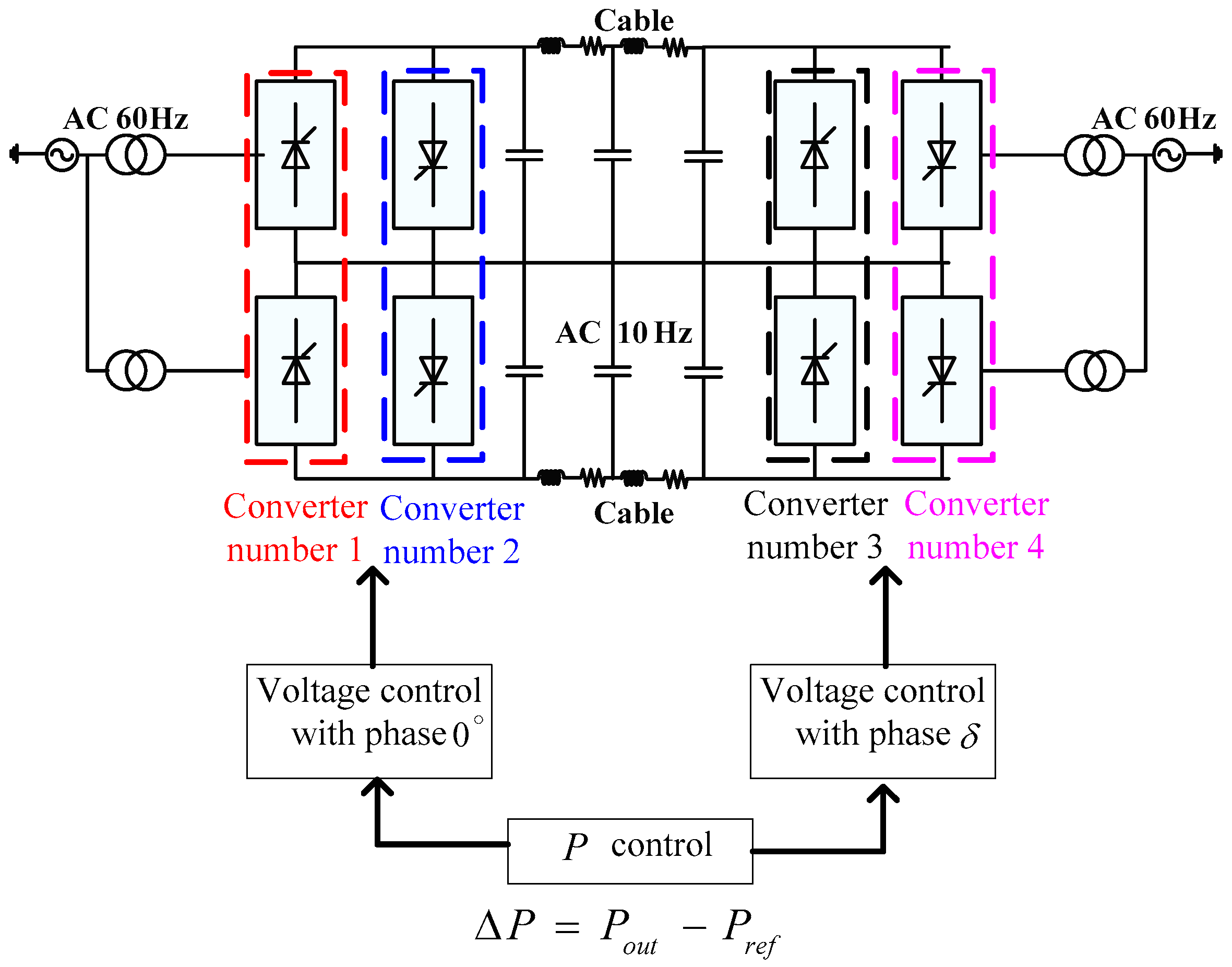
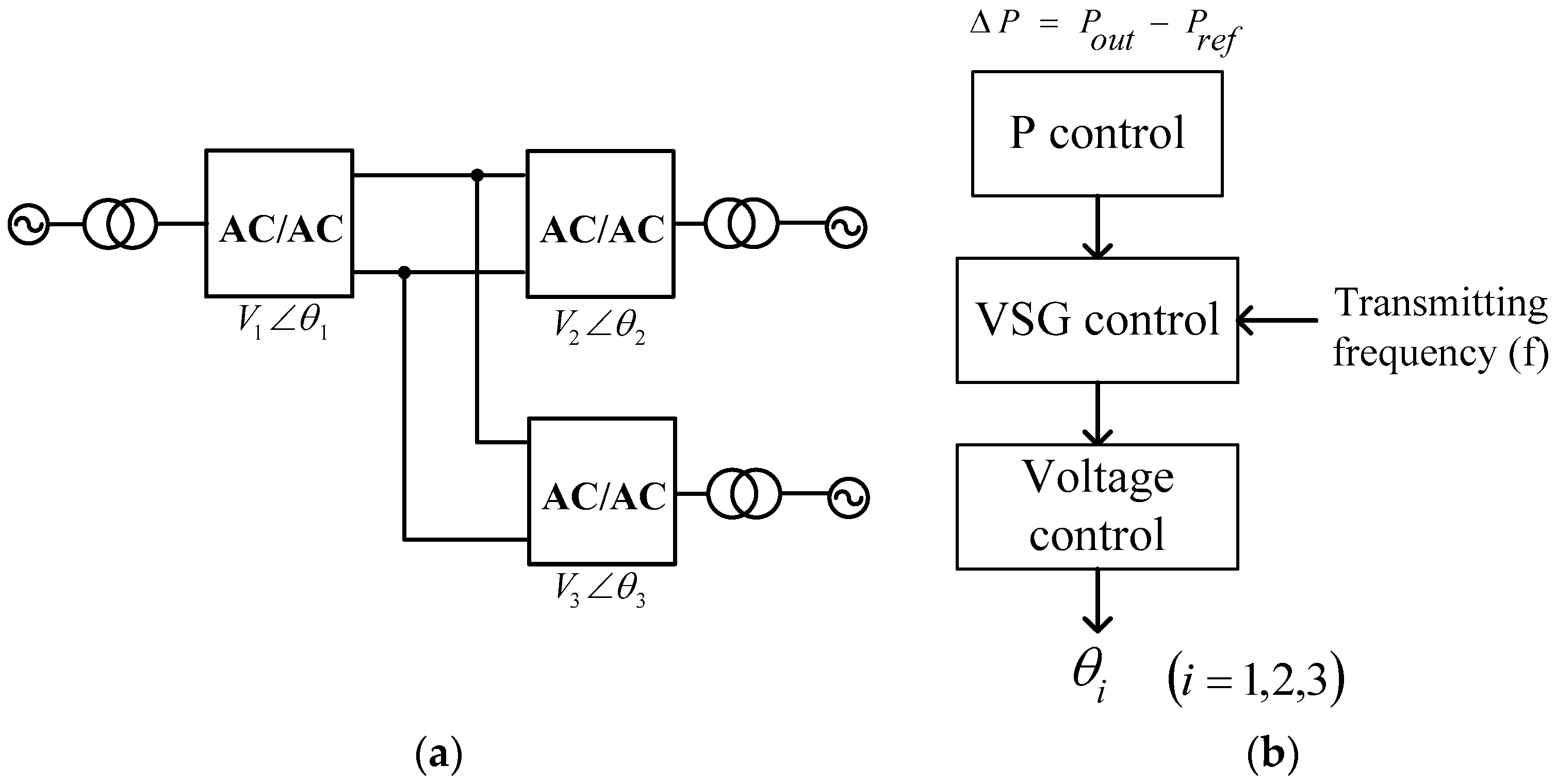
Here, control strategies are applied to both terminals of the cycloconverters. Power control, as shown in 
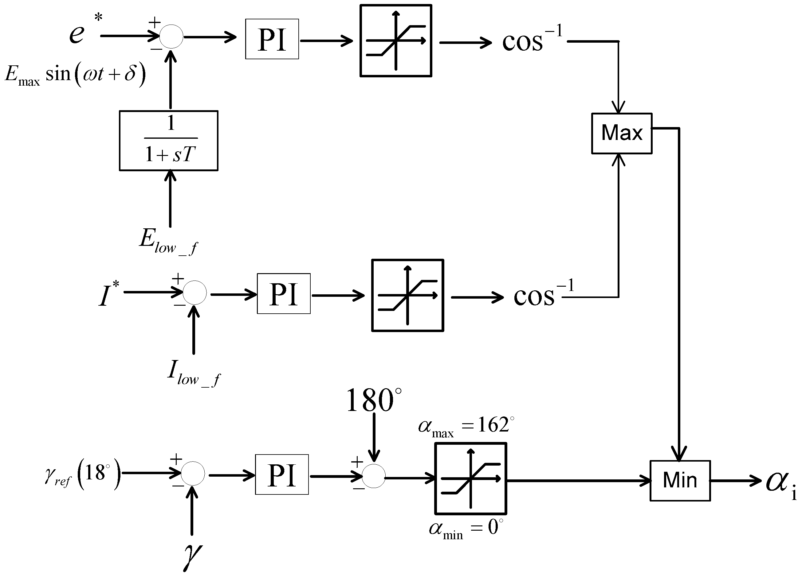
Figure 10, is used to generate a phase difference δ between two terminals following the power reference. Furthermore, voltage control, as shown in Figure 11, works with a phase difference angle to generate a firing angle α i , where i = 1, 2, 3, … is the number of the converter. In case of over current, the current limiter/control will operate to protect the devices in the system. Extinction angle control is also applied to this control scheme for preventing commutation failure in converters. Details of the control scheme are shown in [9]. By applying this control method to the system, Figure 12 shows the layout of the proposed control scheme with the phase difference set at 0° on one side of the converter.

5. Simulation Results

5.1. Simulated System

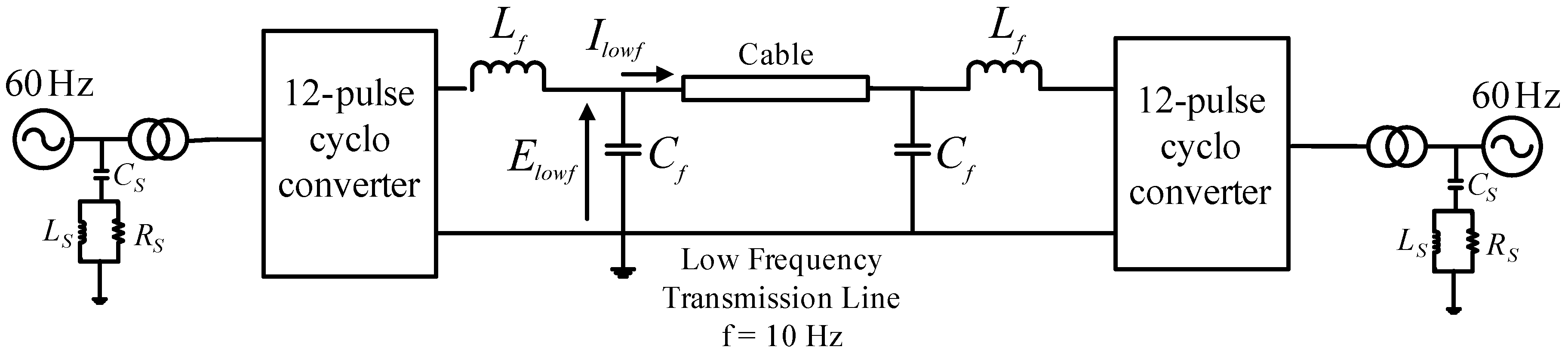
To demonstrate the validity of the proposed LFAC system, simulations have been carried out using the tool of the PSCAD/EMTDC software for an LFAC system as shown in Figure 13. The maximum power transfer is rated at 1400 MW, and the transmission distance is 500 km. The system parameters are listed in Table 1. The transmission power cable is modeled by cascading 50 sections of model cable. Considering low frequency transmission decreases losses in the transmission line, however, too small a value may affect the response time of the system as mentioned in [5]. For a transmission frequency at 10 Hz the delay at the power reversal point is only 0.1 s, and this frequency is used for transmitting power to the transmission target at 500 km distance, so 10 Hz is chosen for this system.
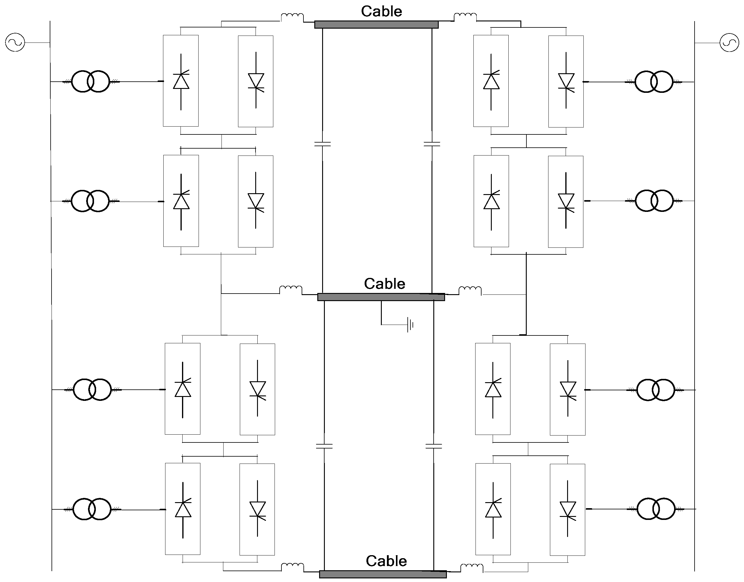
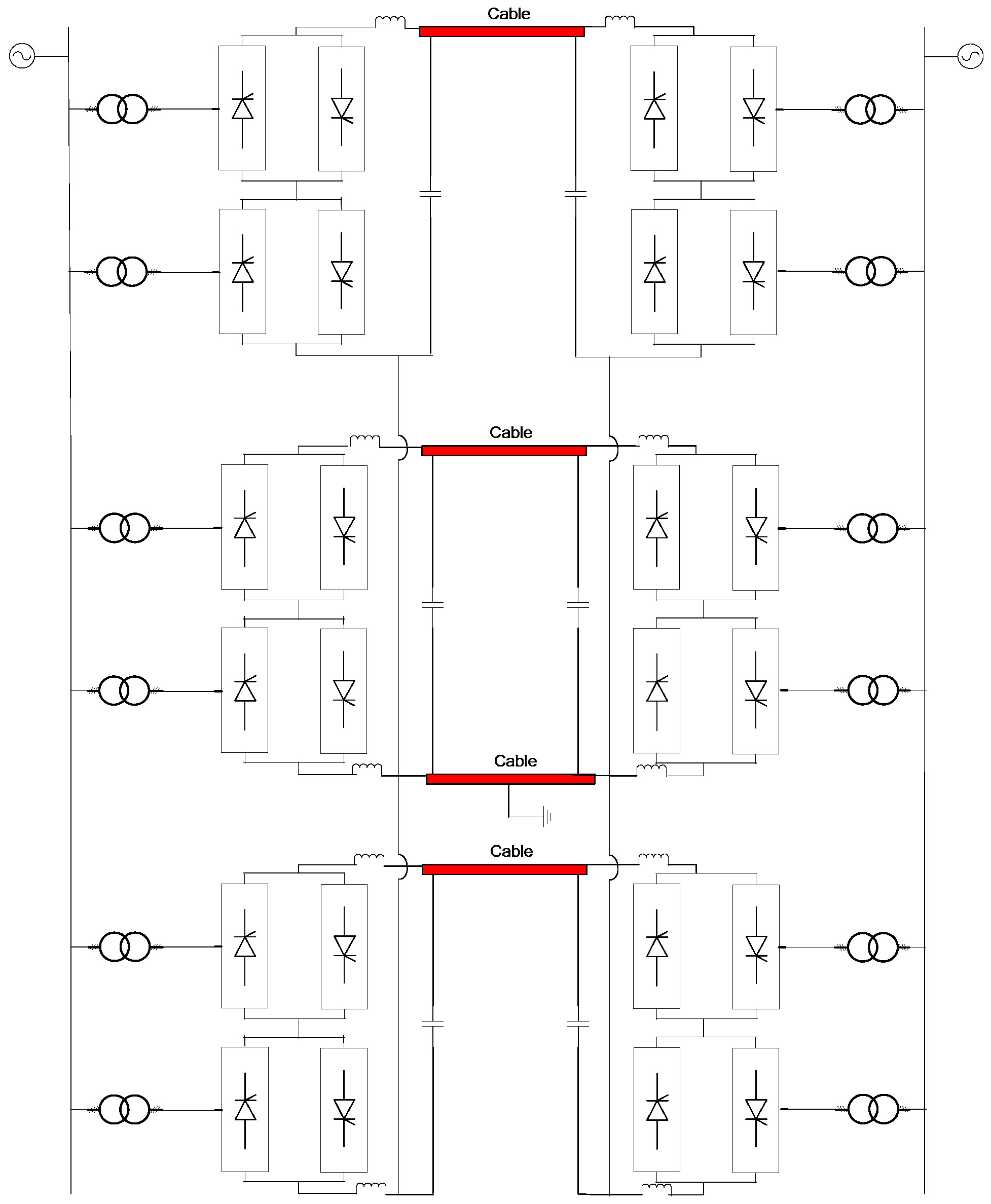
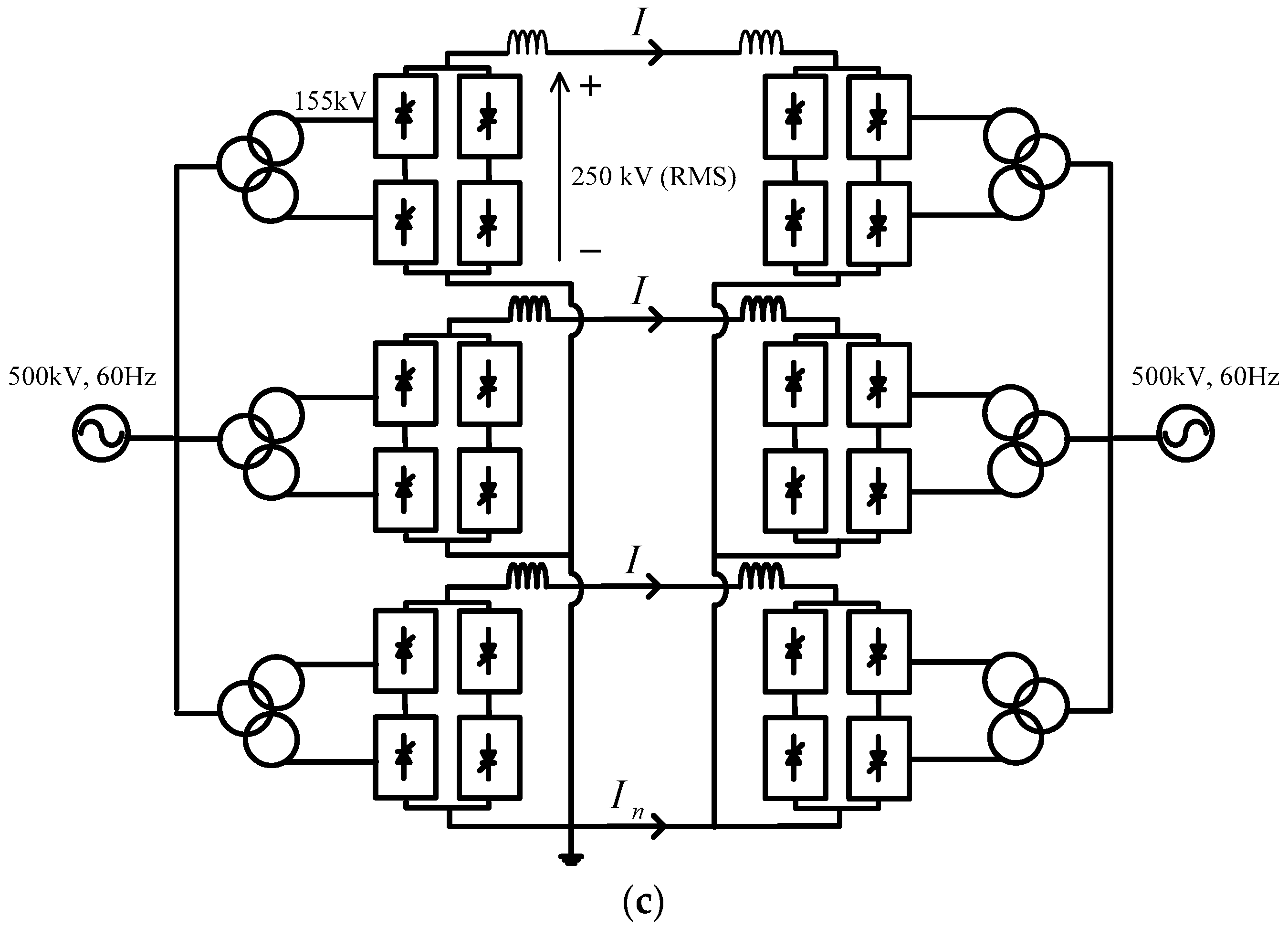
For the operations of this system, each side consists of three phase (Y-∆) and (Y-Y) transformers and two sets of 12-pulse ac-ac converters connected to the power cable. At the sending point (terminal), the cycloconverters work as a frequency converters changing from the utility ac input voltage at 60 Hz to low frequency during power transmission via the cables. At the receiving terminal, another set of cycloconverters works as frequency converters by changing the low frequency to 60 Hz of ac voltage. This procedure can be performed by the proposed configurations as stated in Section 3.
The filters on both sides of the system are low pass filters for receiving the generated ripples and undesirable harmonics from the transmission system. Knowing this fact one can calculate the filter parameters concerning the switching frequency of the power electronics converters.
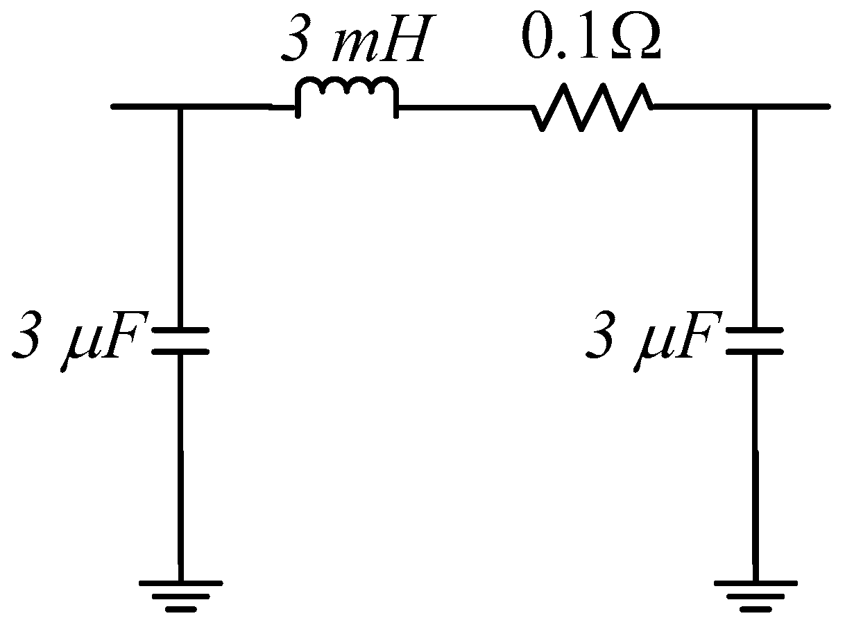
The length of cable is 500 km and transmission frequency is set at 10 Hz for the simulation. The cable model with nominal parameter values is shown in Figure 14.
This cable model is used in all proposed low frequency transmission system configurations. The cable model parameters can be calculated from Equation (2) [10], and the transmission power cable is modeled by using single-core crosslinked polyethylene XLPE underground power cable from ABB (Power and automation technologies, Zurich, Switzerland) with the parameters values of D = 139.2, d = 112.8 and ε s = 2.3 for the XLPE:
C    = 0.02413 ε s log 10 D / d = 0.6 ( μ F / k m ) L     = 0.05 + 0.4605 log 10 D r ( m H / k m ) = 0.3 ( m H / k m ) R a c = 0.0164 ( Ω / k m )
where D is outside diameter of the insulation, and d is inside diameter of the insulation.

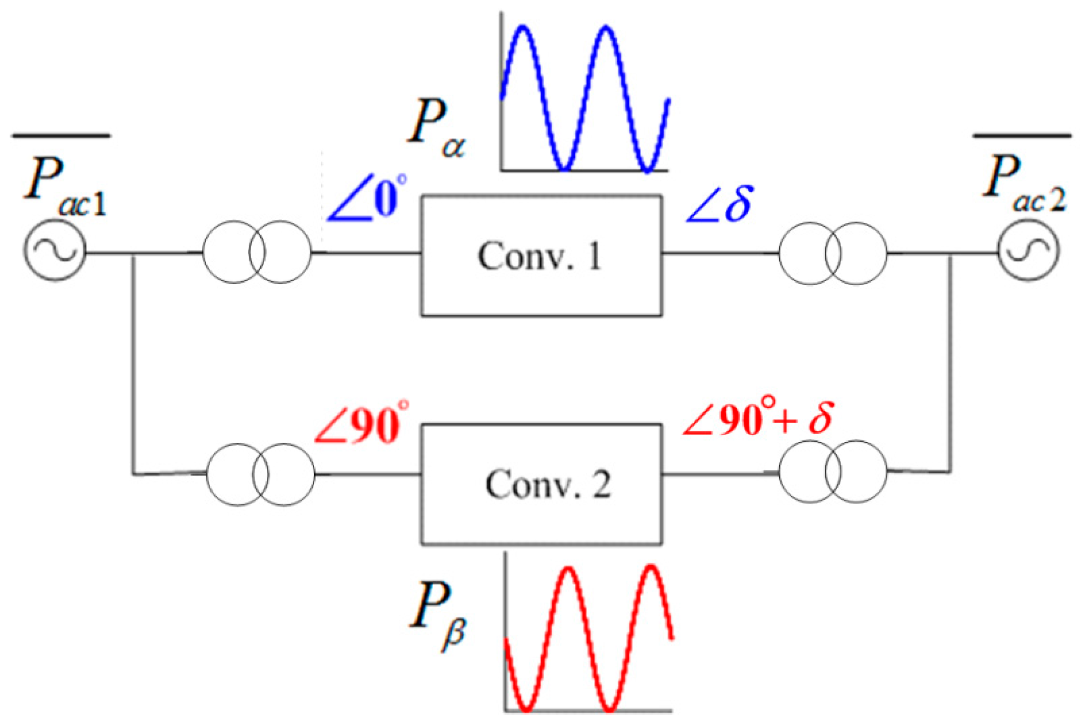
5.2. Power Fluctuation

In the performed low frequency ac transmission system, several types of phase number can be operated for transmitting power. As mentioned previously in the configuration section, single-phase, two-phase and three-phase types are considered for choosing the most suitable system for this transmission system.
To consider the application on three types of LFAC transmission system, the simulation is performed with the parameters given in Table 1. The simulation results are given for both the low frequency and line frequency sides.
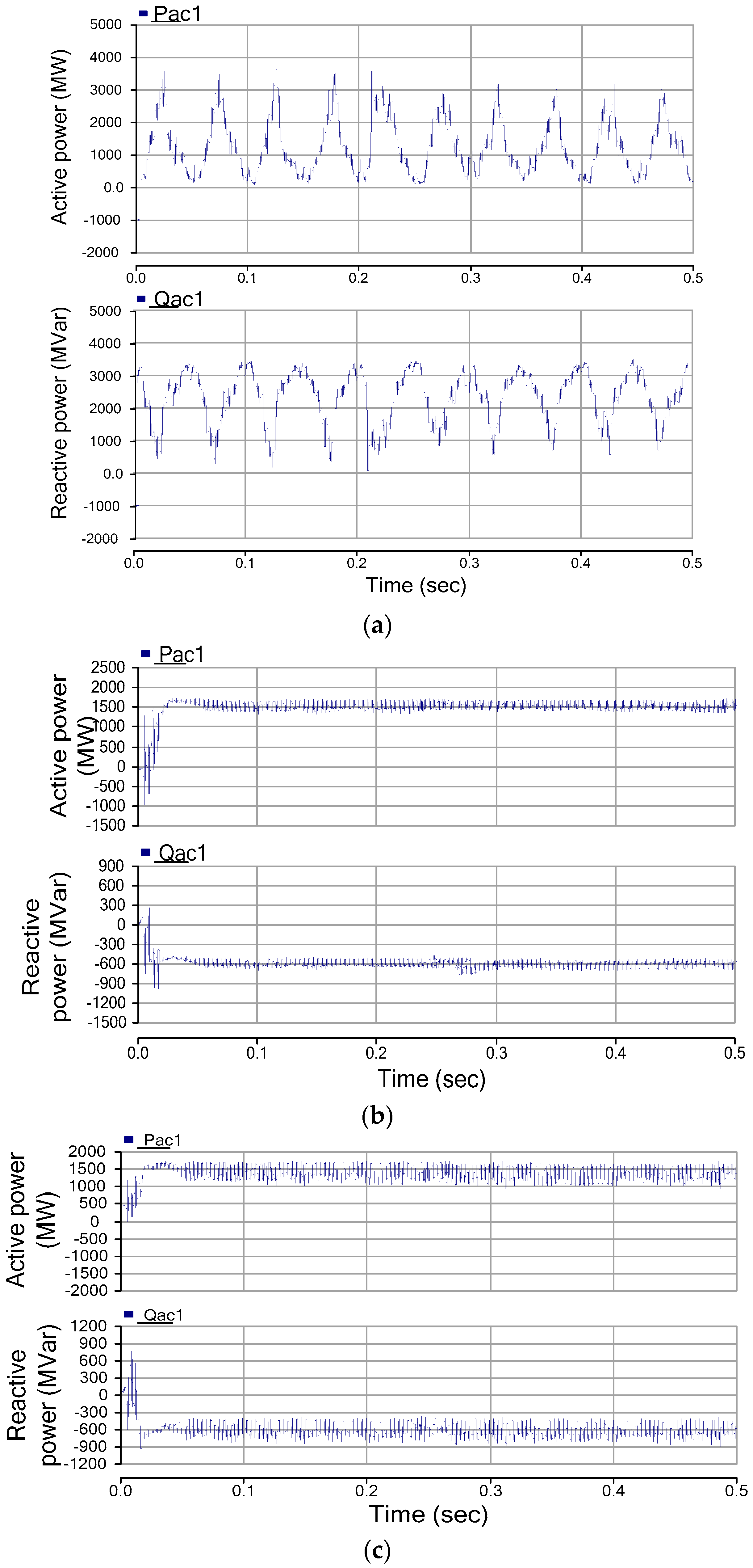
The reference transmission frequency of 10 Hz and reference amount of power of 1400 MW is considered in the transmission system. From the simulation results, Figure 15 shows the active ( P a c 1 ) and reactive power ( Q a c 1 ) waveforms on the line frequency side of the single-phase, two-phase and three-phase configurations, respectively.
As a result, the single-phase system has a fluctuation in power, while the two-phase and three-phase ones do not show any fluctuation on the line frequency side. From the line frequency side point of view, the single-phase system obviously has more fluctuation than the other systems. The two-phase and three-phase systems have constant active and reactive power, without fluctuation.

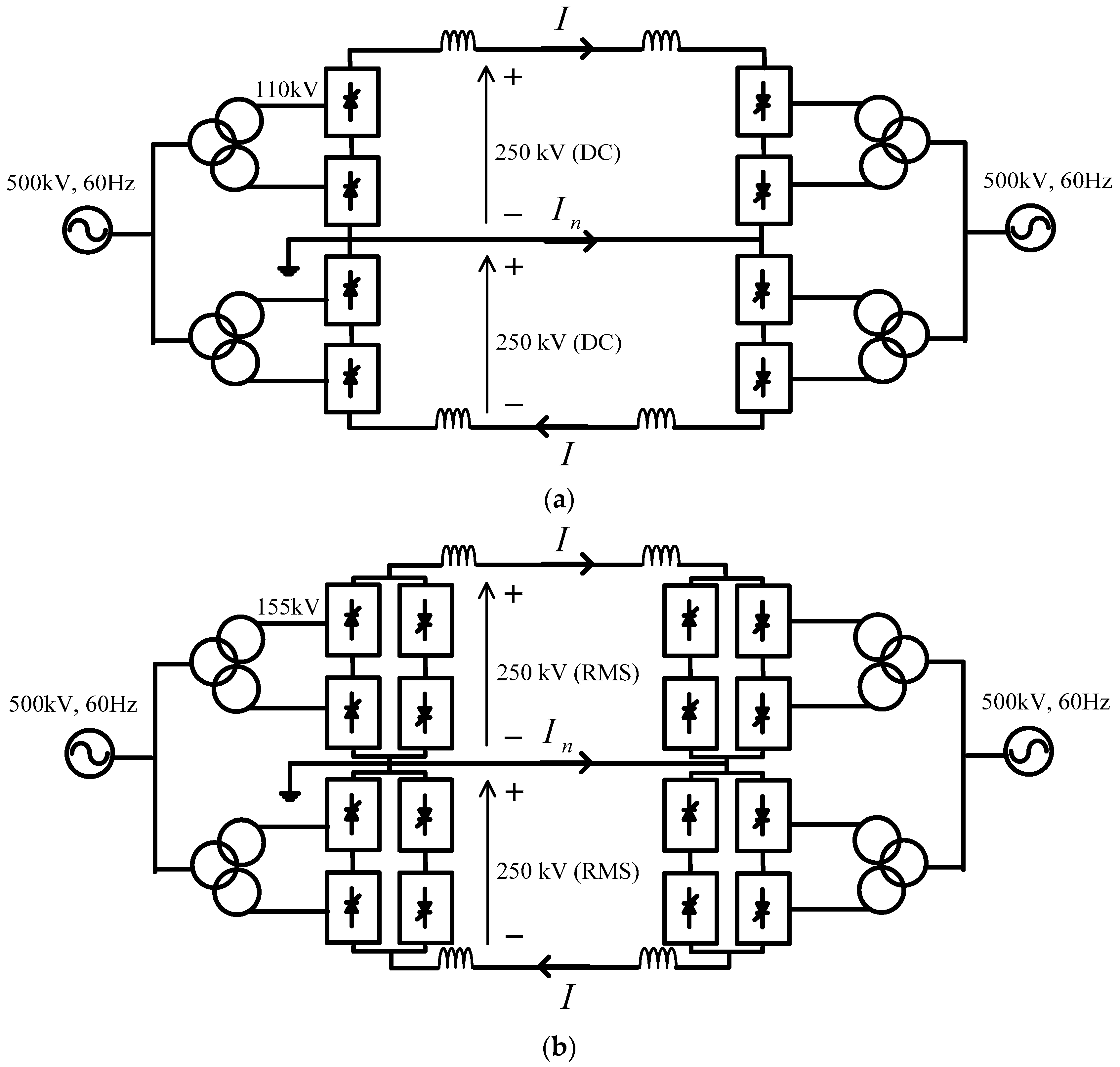
5.3. Ratings of Valves and Transmission Line

With the same transmitting rated power and transmission distance (500 km), the comparison results are shown in Table 2 and Table 3. Table 2 shows the results of valve peak voltage, number of valves per station, valve peak current and average current of LCC-HVDC and three types of LFAC by using valve voltage and DC current of LCC-HVDC system as a based voltage and current. Table 3 shows the results of comparison for transmission line and neutral line currents. The comparison results are obtained by the calculation from Equation (3) for the HVDC and Equation (4) for the LFAC system with the assumption of the same transmitting power for all cases. 
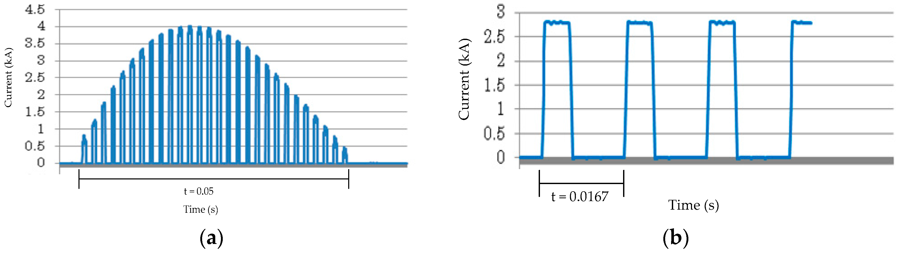
Figure 16 illustrates the overall configuration applied for this evaluation. The output waveform of thyristor current, as shown in Figure 17 can confirm the calculation results.
The calculation formulas for HVDC are as follows:
I p e a k = I d c = I r m s I a v g = I d c 3 I n = 0
where, I p e a k : Valve peak current; I d c : Current on DC side; I r m s : Root mean square (RMS) current on DC side; I a v g : Average current on valve; I n : Neutral current.
The peak and average currents for LFAC system are given by:
I p e a k = 2 I r m s I a v g = 1 2 π 0 π 2 I r m s sin θ d θ      = 2 π I r m s
where, I p e a k : Valve peak current; I r m s : RMS current on low frequency side; I a v g : Average current on low frequency side.
From the comparison results given in Table 2 and Table 3, it can be seen that the LFAC and LCC-HVDC have the same valve voltage RMS value. Three-phase type LFAC has the lowest value of average current, thus leading to low power losses during operation. This configuration also has the lowest RMS current of transmission lines, which affects the size and cost of transmission line in the system. However the numbers of valve devices are the largest compared to the other systems, which negatively affects the size and cost of the frequency converter station. In the case of a two-phase system, it has the same number of devices as the single-phase type, but the average current is lower than in the LCC-HVDC system, the number of cables is the same as LCC-HVDC and the single-phase system, while the neutral line current is large, which is the main demerit of this system compared to the others. For these reasons, two-phase and three-phase systems should be chosen considering the length of transmission. For longer transmission systems, a three-phase system is more suitable.

5.4. Power Reversal and System Disturbance Simulation Results

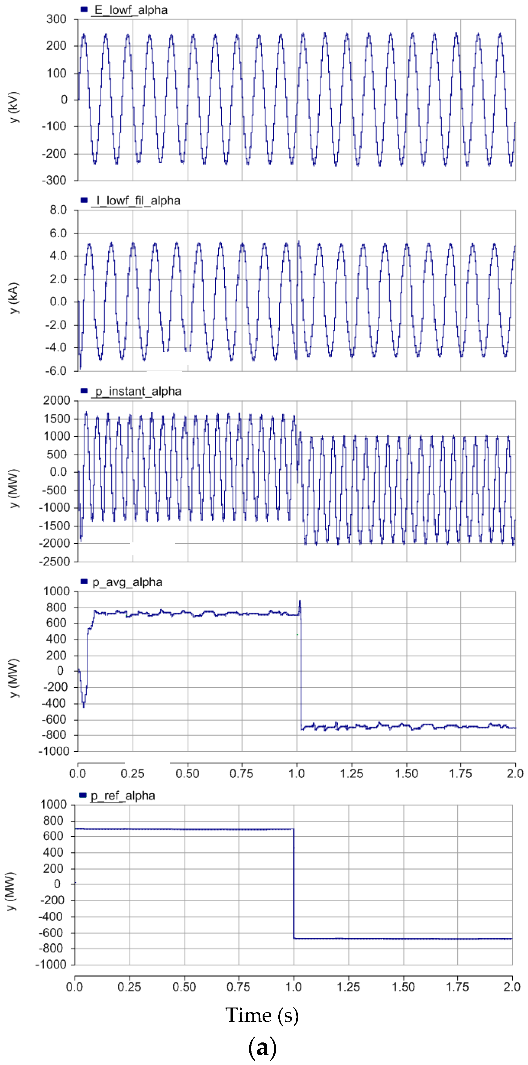
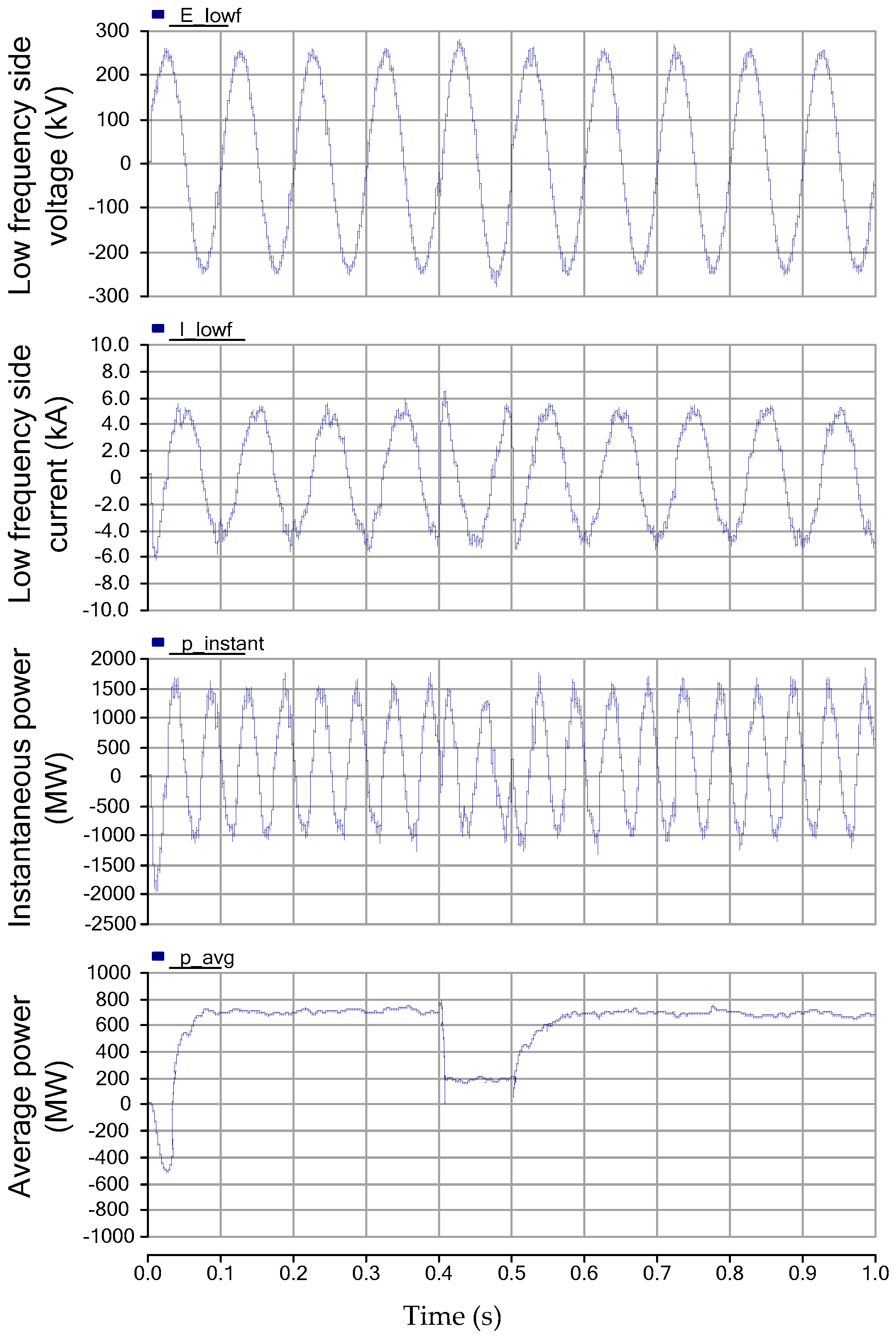
As for two-phase LFAC, the reference frequency used is 10 Hz, the transmitted reference power is 700 MW. Figure 18a shows waveforms of voltage E_lowf, current I_lowf, instantaneous power p_instant, average power, p_avg and reference value of transmitted power p_ref on the low frequency side. The power reversal starts at t = 1. 
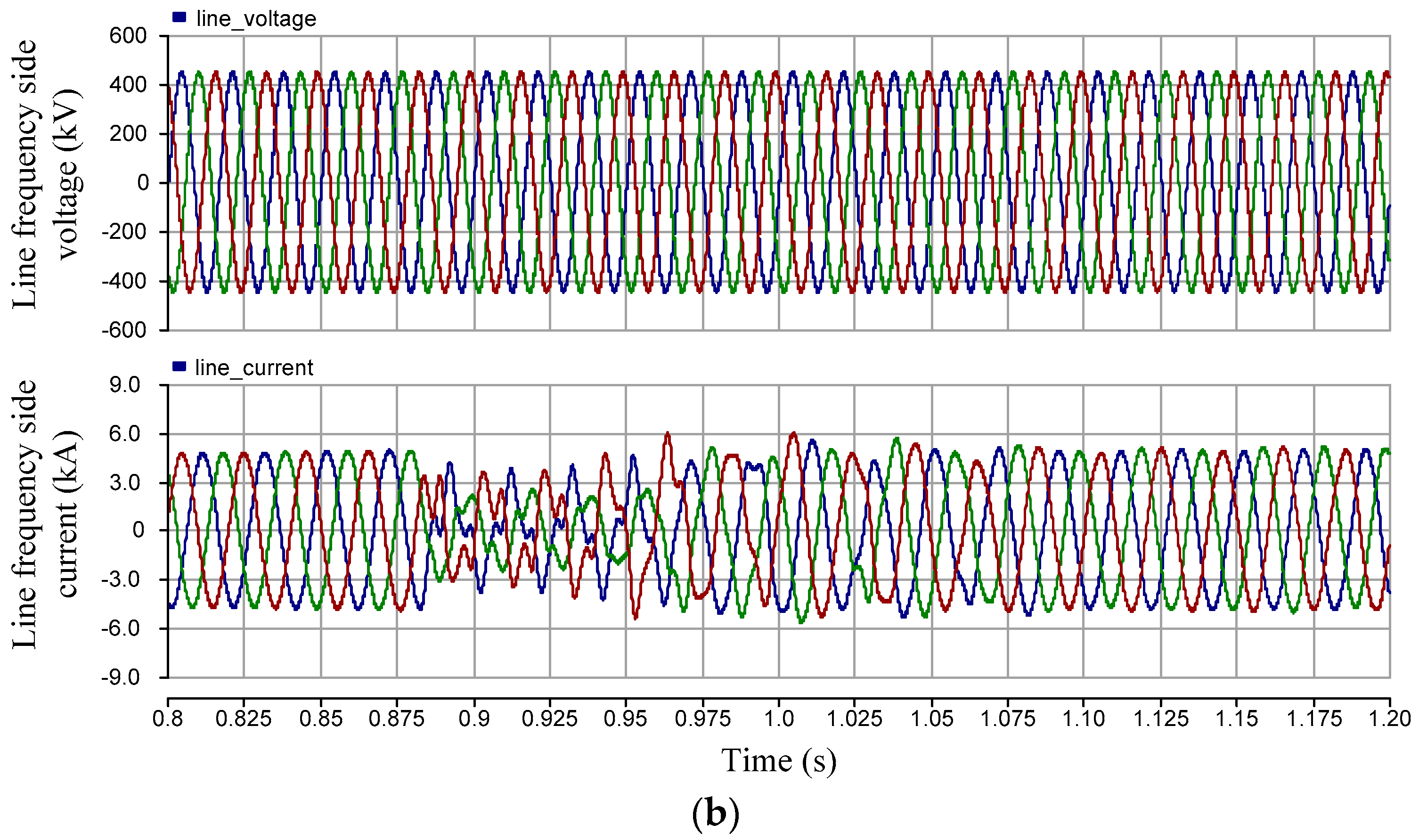
Figure 18b shows voltage and current waveforms on the line frequency side (60 Hz) at around 1.0 s, which is near the transient change of the power reference. With these simulation results, it can be confirmed that the proposed control scheme properly works for the LFAC transmission system.
To evaluate the system response in the presence of faults or disturbances, a step change in reference power is applied. In normal operation the system is operating at a power reference of 700 MW, then the reference power is suddenly changed to 200 MW for one cycle. As can be seen in Figure 19, the closed-loop system remains stable and returns to normal operation in a short time.

6. Conclusions

This paper explains the features of three configurations of the LFAC and LCC-HVDC. Focusing on the application of multi-terminal systems, three low frequency ac transmission system configurations using cycloconverters with the same system scale have been presented for studies on the circuit operation and suitable number of operating phases. There are three main important points to be concluded as follows:
  • The merits of LFAC over HVDC transmission system were explained with multi-terminal application which is unnecessary to use additional mechanical switches to change power flow direction and no need for communication link to synchronize among terminals.
  • Configuration for three types of LFAC system were studied and verified by simulation results with the same condition and system parameters.
  • LFAC is feasible on the multi-terminal system. To choose the most suitable configuration of LFAC operation, the three configurations of LFAC have been compared. The results review that single-phase system has the obvious power fluctuation on line frequency system. Two-phase and three-phase systems can be considered as the most suitable configurations for multi-terminal LFAC system. According to the comparison results in Section 5.3, two-phase system has a strong point for less number of devices but has a weak point for a large neutral line current. On the other hand, three-phase system has the advantage on valve peak and average current but it contains large number of devices. For longer transmission, three-phase system has advantage due to less copper amount for the transmission lines.
Further research towards LFAC transmission system, analysis of voltage and current transient and faults analysis are still needed. All these issues require further investigation.

Author Contributions

Achara Pichetjamroen performed calculation, simulation of system, comparison of system configurations and wrote the paper. Toshifumi Ise as research supervisor provided guidance and key suggestions, participated in proposing the basic ideas of the system configurations and control scheme, and helped in writing the paper.

Conflicts of Interest

The authors declare no conflict of interest.

Nomenclature

P α and P β Power on upper and lower part on low frequency side of two-phase system
V L F Voltage on low frequency side
I L F Current on low frequency side
C Cable capacitance
L Cable inductance
D Outside diameter of insulation
d Inside diameter of insulation
P a c Active power on line frequency side
Q a c Reactive power on line frequency side

References

  1. Lescale, V.; Kumar, A.; Juhlin, L.-E.; Bjorklund, H.; Nyberg, K. Challenges with multi-terminal UHVDC transmissions. In Proceedings of the Power System Technology and IEEE Power India Conference, New Delhi, India, 12–15 October 2008.
  2. Funaki, T.; Matsuura, K. Feasibility of the low frequency AC transmission. In Proceedings of the Power Engineering Society Winter Meeting, Singapore, 23–27 January 2000.
  3. Achara, P.; Ise, T. Power control of low frequency AC transmission system using cycloconverters with virtual synchronous generator control. In Proceedings of the Industrial Electronics Society Conference, Yokohama, Japan, 9–12 November 2015.
  4. Slade, P.G.; Smith, R.K. A comparison of the short circuit interruption performance using transverse magnetic field contacts and axial magnetic field contacts in low frequency circuits with long arcing times. In Proceedings of the Discharges and Electrical Insulation in Vacuum International Symposium, Yalta, Crimea, 27 September–1 October 2004.
  5. Chen, H.; Johnson, M.H.; Aliprantis, D.C. Low-frequency AC transmission for offshore wind power. IEEE Trans. Power Deliv. 2013, 28, 2236–2244. [Google Scholar] [CrossRef]
  6. Mau, C.; Rudion, K.; Orths, A.; Eriksen, P.B.; Abildgaard, H.; Styczynski, Z. Grid connection of offshore wind farm based DFIG with low frequency AC transmission system. In Proceedings of the Power and Energy Society General Meeting, San Diego, CA, USA, 22–26 July 2012.
  7. Nakagawa, R.; Funaki, T. Kenji Matsuura Installation and control of cycloconverter to low frequency AC power cable transmission. In Proceedings of the Power Conversion Conference, Osaka, Japan, 2–5 April 2002.
  8. Wang, X.; Cao, C.; Zhou, Z. Experiment on fractional frequency transmission system. IEEE Trans. Power Syst. 2006, 21, 372–377. [Google Scholar]
  9. Bevrani, H.; Ise, T.; Miura, Y. Virtual synchronous generators: A survey and new perspectives. Int. J. Electr. Power Energy Syst. 2014, 54, 244–254. [Google Scholar] [CrossRef]
  10. Short, T.A. Underground distribution. In Electric Power Distribution Handbook, 2nd ed.; Grigsby Leo, L., Ed.; CRC Press: Boca Raton, FL, USA, 2003; Volume 3, pp. 167–168. [Google Scholar]
Figure 1. Configuration of the line-commutated converter based multi-terminal HVDC (LCC-MTDC).
Energies 09 00687 g001
Figure 2. Configuration of the voltage-source converter based multi-terminal HVDC (VSC-MTDC).
Energies 09 00687 g002
Figure 3. Configuration of the line-commutated converter based multi-terminal LFAC (LCC-MTLF).
Energies 09 00687 g003
Figure 4. Control scheme of the VSC-MTDC.
Energies 09 00687 g004
Figure 5. Configuration of the LCC-MTLF: (a) Power flow configuration; (b) VSG control concept.
Energies 09 00687 g005
Figure 6. Configuration of single-phase low frequency ac transmission system (LFAC).
Energies 09 00687 g006
Figure 7. Power fluctuation of single-phase LFAC transmission system.
Energies 09 00687 g007
Figure 8. Power fluctuation of two-phase LFAC transmission system.
Energies 09 00687 g008
Figure 9. Configuration of three-phase low frequency ac transmission system.
Energies 09 00687 g009
Figure 10. Control scheme of transmitting power control.
Energies 09 00687 g010
Figure 11. Control scheme of LFAC transmission system.
Energies 09 00687 g011
Figure 12. Layout of control system for LFAC system.
Energies 09 00687 g012
Figure 13. The simulated LFAC system configuration.
Energies 09 00687 g013
Figure 14. Cable model for the simulation.
Energies 09 00687 g014
Figure 15. Line frequency side simulation results: (a) Single-phase system; (b) Two-phase system; (c) Three-phase system.
Energies 09 00687 g015
Figure 16. Configurations for valve and transmission line rating current: (a) High voltage direct current HVDC; (b) Single-phase and two-phase; (c) Three-phase.
Energies 09 00687 g016aEnergies 09 00687 g016b
Figure 17. Thyristor current of LFAC and HVDC system: (a) LFAC; (b) HVDC.
Energies 09 00687 g017
Figure 18. Simulation result of two-phase LFAC transmission system of power reversal: (a) Low frequency side (10 Hz); (b) Line frequency side (60 Hz).
Energies 09 00687 g018aEnergies 09 00687 g018b
Figure 19. Simulation result of a sudden change of reference power.
Energies 09 00687 g019
Table 1. Parameters of the simulated system.
ParameterValue
Maximum power transfer1400 MW
Grid voltage500 kV
Line frequency60 Hz
Transmitting frequency10 Hz
Transformer500 kV/110 kV
L f 1 mH
C f 0.02 F
L S 14 mH
C S 1.55 µF
R S 100 Ω
Table 2. Comparison of valve rating.
Valve RatingLCC-HVDCLFAC
Single-PhaseTwo-PhaseThree-Phase
Valve RMS voltage1 pu1 pu1 pu1 pu
Valves/station24 valves48 valves48 valves72 valves
Valve peak current ( I p e a k )1 pu 2 pu 2 pu 2 3 2   pu (=0.94)
Valve average current ( I a v g ) 1 3   pu 2 π × 1 3   pu (=0.15) 2 π × 1 3   pu (=0.15) 2 π × 2 3   × 1 3  pu (=0.1)
Table 3. Comparison of transmission line rating.
Current RatingLCC-HVDCLFAC
Single-PhaseTwo-PhaseThree-Phase
Current of transmission line in RMS ( I r m s )1 pu × 2 lines1 pu × 2 lines1 pu × 2 lines 2 3   pu   × 3   lines
Neutral line current in RMS ( I n )00 2 pu0

