Article

Energy Management of an Off-Grid Hybrid Power Plant with Multiple Energy Storage Systems

1
Department of Engineering, Niccolò Cusano University, via Don Carlo Gnocchi 3, 00166 Rome, Italy
2
Department of Engineering, University of Rome Tor Vergata, via Orazio Raimondo 18, 00173 Rome, Italy
*
Author to whom correspondence should be addressed.
Energies 2016, 9(8), 661; https://doi.org/10.3390/en9080661
Submission received: 1 June 2016 / Revised: 3 August 2016 / Accepted: 4 August 2016 / Published: 19 August 2016

Abstract

:
In this paper, an off-grid hybrid power plant with multiple storage systems for an artificial island is designed and two possible strategies for the management of the stored energy are proposed. Renewable power sources (wind/solar technologies) are used as primary power suppliers. A lead-acid battery pack (BAT) and a reversible polymer electrolyte fuel cell are employed to fulfill the power demand and to absorb extra power. The reversible fuel cell allows reducing costs and occupied space and the fuel cell can be fed by the pure hydrogen produced by means of its reversible operation as an electrolyzer. A diesel engine is employed as backup system. While HOMER Pro® has been employed for a full-factorial-based optimization of the sizes of the renewable sources and the BAT, Matlab/Simulink® has been later used for simulating the plant operation and compare two possible power management control strategies. For the reversible fuel cell sizing, a sensitivity analysis has been carried out varying stack and hydrogen tank sizes. The final choice for plant configuration and power management control strategy has been made on the basis of a comparative analysis of the results, aimed at minimizing fossil fuel consumption and CO2 emissions, battery aging rate and at maximizing the power plant overall efficiency. The obtained results demonstrate the possibility of realizing a renewable power plant, able to match the needs of electrical power in a remote area, by achieving a good integration of different energy sources and facing the intermittent nature of renewable power sources, with very low use of fossil fuels.

Graphical Abstract

1. Introduction

TUNeIT (TUNisia and ITaly) project—part of the MedTracking research program carried out by the Network of Schools of Engineering in the Mediterranean RMEI (Réseau des Ecoles des Ingenieurs Méditerranéen) [1]—proposes to link the Sicilian coast to the Tunisian one, for a total length of about 140 km, by creating five bridges, with the same characteristics of the one of the Messina project, starting from and arriving to four artificial islands. Beyond acting as structural elements, these islands are aimed at providing all the services necessary for the operation of the infrastructure and are thought to be equipped with electrical power-demanding facilities for tourists—such as gas stations, hotels and/or restaurants. Power supply in remote areas is in general a big challenge, but in this case, being artificial islands, the minimization of its environmental impact, especially in terms of pollutant and greenhouse gases emissions, is even more crucial. This, together with rising of energy demand and sudden fluctuations of fossil fuels price, makes green power generation systems the most suitable technologies to be employed for the specific application [2], especially because of the great wind and solar potentials typical of the Mediterranean area [3].
The greatest problem to be faced by an off-grid wind/solar system is matching the intermittence of the power supplied by the renewable energy sources with the dynamic load demand of the consumers, which cannot be foreseen, especially when past data are not available. Unmet electrical needs and excess power production can frequently occur and solutions to this are: combination of different renewable energy sources—such as solar and wind sources—and addition of energy storage systems (ESS) into the power plant, especially when connection to the electrical grid is not possible or expensive to realize [4].
Several energy storage systems have been proposed for these kind of hybrid plants, such as pumped hydro storage systems (PHSS) [5], compressed air storage systems (CAES) [6] and hydro systems coupled to compressed air ones [7], but lead-acid batteries and hydrogen storage systems are the most commonly employed because of their ability to “co-operate” [8,9]. In fact, batteries are better suited for short-term energy storage for their fast charging/discharging capacity and high round-trip efficiency, while hydrogen can be effectively used for long-term energy storage, for its high mass energy density and the possibility to prevent the energy losses related to the self-discharge of batteries. For hydrogen storage and usage, a reversible polymer electrolyte membrane fuel cell (RePEM) can be employed to allow reducing costs and occupied space. Nevertheless, if on one hand the long-term storage reduces the wear of the reversible fuel cell thanks to the less frequent activations and deactivations, on the other hand, the frequent charging/discharging cycles of batteries can significantly increase their aging rate. Therefore, a proper sizing and power management strategy must be applied to the specific plant in order to take into account all these conflicting behaviors. Although the plant aims at a 100% sustainable operation, a diesel internal combustion engine must be considered as backup system, in order to cope with a possible lack of energy, related to the unpredictable availability of the energy sources.
In this paper, a hybrid power plant is designed and two possible power management strategies are proposed and compared in terms of fossil fuel usage, battery aging and RePEM size. The different strategies are compared in terms of overall plant efficiency, fossil fuel consumption and CO2 emissions and battery aging rate.
For the power plant sizing, HOMER Pro® Software (HOMER Energy LLC, Boulder, CO, USA) tool is employed [10], resulting in a slight oversize of wind and solar power converters, in order to produce as much power as possible during windy and sunny days, while a sensitivity analysis has been performed to find a size of the RePEM which allows a trade-off between fossil fuel usage by the diesel generator and battery aging rate.
A rule-based approach has been implemented for the plant power management strategies because of its reliability, and the strategies have been reproduced and verified by means of a self-made simulation tool developed in Matlab/Simulink® r2014a (The Mathworks, Inc., Natick, MA, USA). In both the proposed strategies, wind and solar energy sources are used as primary power suppliers, while the RePEM, together with the BAT, are employed to fulfill the power demand—when the power supplied by the renewable power generators is not sufficient—or to absorb excess power, when available. The BAT is always used as primary energy recovery system, followed by the RePEM in electrolyzer mode if needed, while the extra power demand is satisfied first by the battery and then by the RePEM in fuel cell mode in one case and vice versa in the second case.

2. System Configuration

The proposed power plant should consist of wind turbines (WT), photovoltaic panels (PV), a battery pack, a reversible polymer electrolyte membrane fuel cell (RePEM) and a diesel internal combustion engine (ICE), as shown in Figure 1.

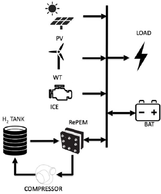
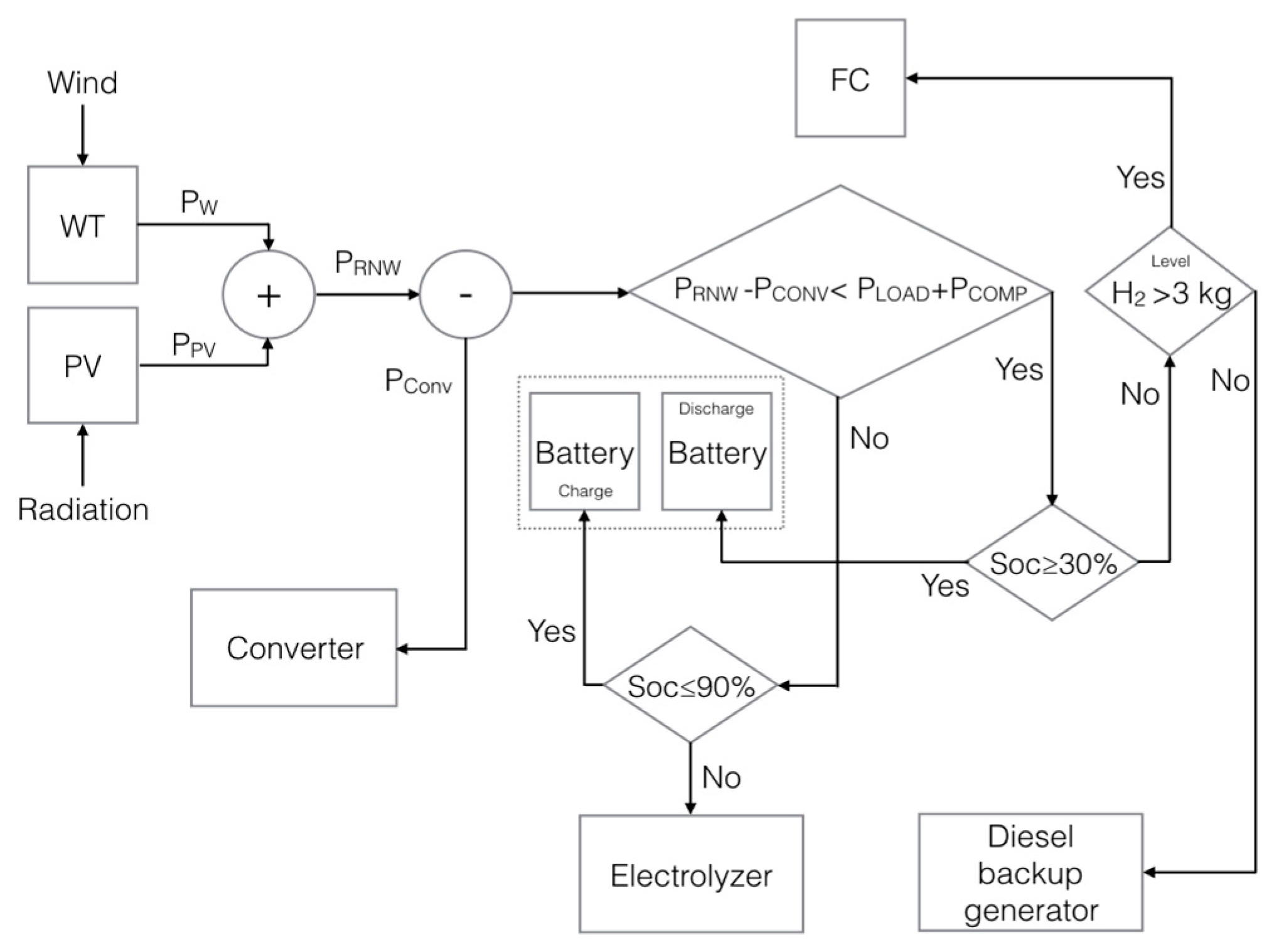
2.1. Component Sizing

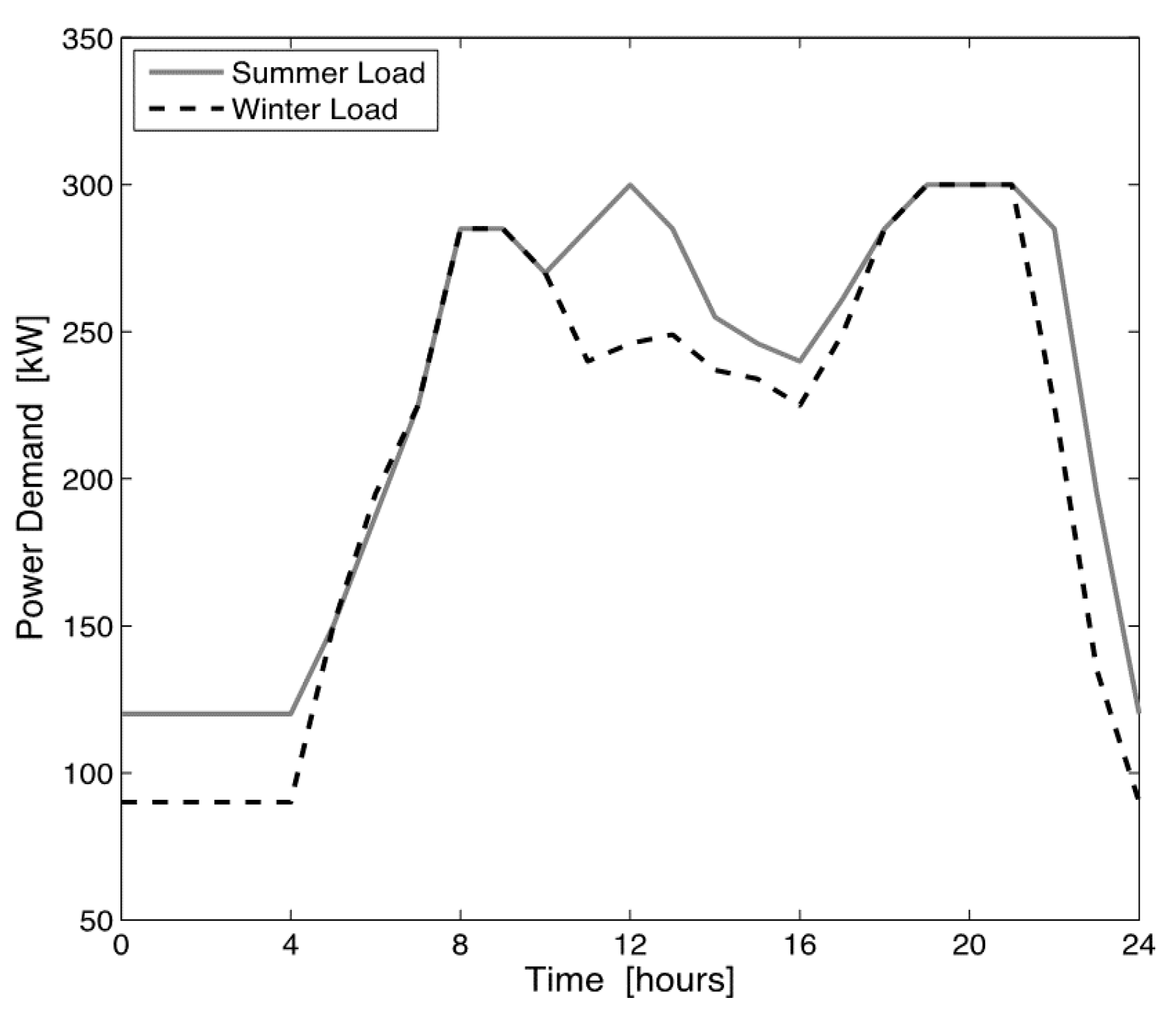
An electrical power demand profile has been assumed in order to reproduce the possible power demand of one of these artificial islands. The project is still on-going, therefore there is no availability of measured data to reproduce real power load profiles. Nonetheless, since these islands will be likely equipped with facilities for tourists, the employed load curves were derived from a past study, realized within a National Operative Program [11], where the power demand of a mid-size hospitality structure, comparable to the one that could be built on the island, was carefully evaluated by in-situ measurements. The resulting profiles are shown in Figure 2, and have been used to represent typical summer and winter daily loads, characterized by a peak power demand of 300 kW and a minimum power of 90 kW during winter and 120 kW during summer.
Number of WT, PV panels and the size of the BAT have been optimized by means of HOMER Pro®, which allows for modeling and sizing each component and for power plant operation analysis. HOMER is one of the most widely used tools for power plant components sizing, having the possibility of combining a great number of renewable energy systems and being able to perform optimizations and sensitivity analyses, which make easier and faster the evaluation of the best system configurations among the many possible [10].
The reversible fuel cell has been sized, a-posteriori, on the basis of a sensitivity analysis, as a trade-off between fossil fuel consumption and initial investment costs, once the plant setup was configured by HOMER. The choice of an a-posteriori sizing of the RePEM has been made to cope with the lack of such a template in HOMER and to use it as a tuning parameter for the power management control strategies, in order to find a trade-off between battery degradation rate and fossil fuel consumption.
HOMER optimizes the plant configuration by applying a full factorial design of experiments and choosing the configuration with the minimum cost of energy, which estimates the installing and operating costs of the system over its lifespan, as already explained in [12].
In the full factorial array definition, the wind turbine rated power has been set equal to 1 MW, and the number of turbines is the result of the optimization. Such a high value for the rated power is a consequence of a mean annual load factor of only 10.2%, i.e., the turbine utilization factor, function of the specific wind speed profile, considered equal to the one available from a weather station located in Mazara del Vallo, Sicily.
The PV array size has been varied between 800 kW and 1.1 MW, by a fixed step of 100 kW. Similar to the wind turbine, these high values of the rated power are dictated by a mean annual load factor of 15.9%, as a function of the solar radiation profile that HOMER itself extracts from given latitude and longitude values, i.e., N 37°33′ latitude and E 12°0′ longitude [13,14,15].
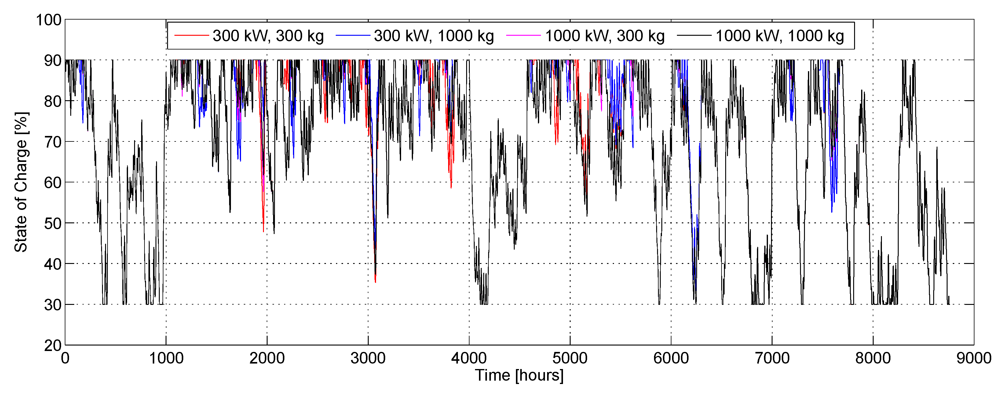
For the BAT, a number of strings in parallel varying in the range of 100–700 has been considered, with a step of 100. A single battery string is composed of 12 cells, set in series, with nominal cell voltage of 2 V, nominal capacity of 3000 Ah and SOC range 30%–90% [16].
The final configuration obtained in the optimization performed with HOMER consists of: 1 wind turbine, 1.1 MW rated power for the PV array and 200 battery strings.
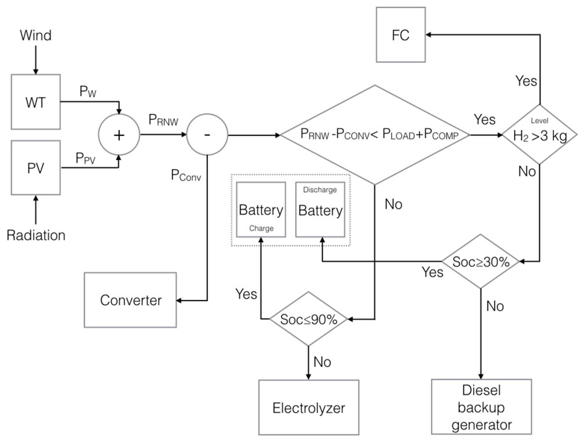
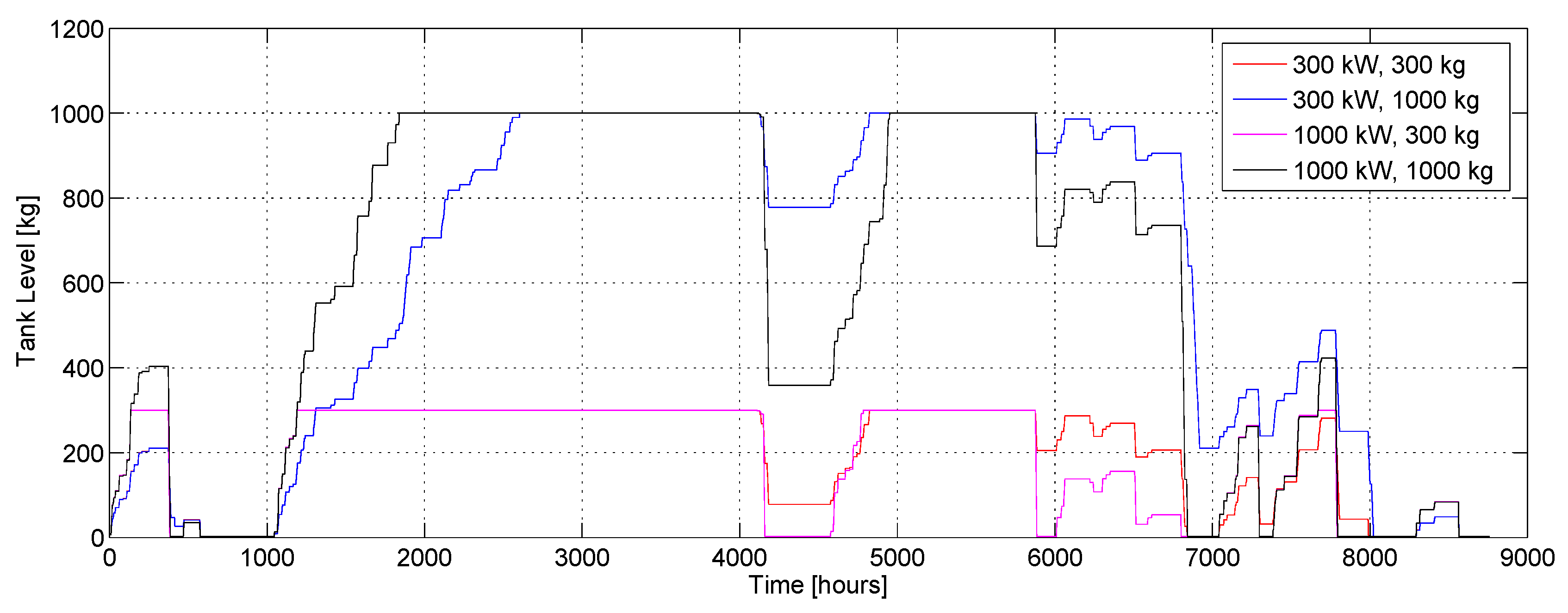
For the reversible fuel cell offline sizing, five scenarios, shown in Table 1, have been considered, varying the maximum stack power and the tank capacity. A fixed volume has been considered in the different scenarios for the tank, therefore different energy consumptions can be ascribed to the compressor in the five cases, affecting the overall efficiency of the power plant.
Finally, for the ICE, being a backup system, it has been sized as to be able to satisfy the peak power demand, i.e., 300 kW. In fact, its usage must cope with failures or it should be used to fulfill power demands higher than the maximum considered.

2.2. Component Modeling

Once the power plant was sized, its operation has been simulated by means of an energy-based quasi-static simulator developed in Matlab/Simulink® environment [17], which includes an equivalent circuit model for the battery operation and battery state of charge dynamics, and a semi-empirical model for the RePEM.
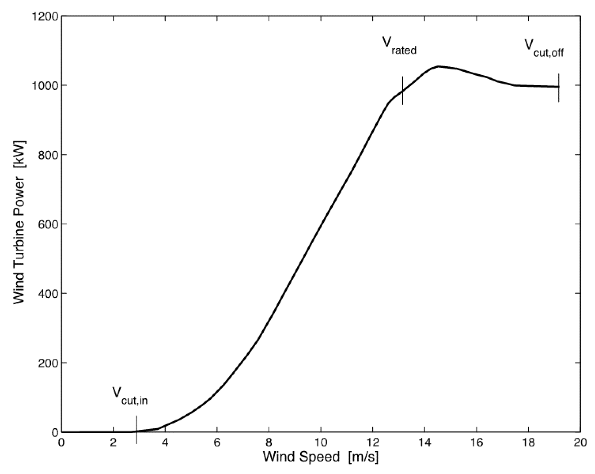
(1) Wind turbine: this component has been modeled as a device which converts wind kinetic power into mechanical power (PW), by means of a user defined wind turbine power curve, shown in Figure 3, for the considered turbine.
The turbine power is obviously a function of wind speed as per Equation (1):
P WT = { 0 , if   V < V cut , in  and  V > V cut , off P WT = 1 2 ρ A T V 3 C p , if   V cut , in < V < V cut , off
where Vcut,in is the cut-in wind speed, i.e., the wind speed at which the turbine starts generating output power; Vcut,off is the maximum allowable wind speed, above which blades damage could occur; V is the wind speed, whose values—collected at a certain anemometer height—are corrected to the turbine hub height; ρ is the air density; AT is the area swept by the blades; and Cp is turbine power coefficient, or rotor efficiency, which also depends on the wind speed. Nevertheless, WT with a rated capacity of about 1 MW or larger are usually equipped with an active stall control mechanism. In such systems, the controller makes the turbine run at maximum efficiency, i.e., maximum power coefficient—until the rated power is reached. Once the wind speed has reached the so-called rated wind speed value, pitch angle is adjusted so that to stall the turbine and limit the output power.
(2) Photovoltaic panels: for the PV array, dependency on temperature has been included as suggested by [19]. The power output from the PV system has been evaluated as:
P P V = I T A PV η PV
where Apv is the PV system area, while ηPV is the panel efficiency, given by:
η PV = η PV , ref [ 1 β ( T C T ref ) ]
where ηpv,ref is the module electrical efficiency at reference cell temperature Tref and at solar radiation flux of 1 kW/m2, while β is the temperature coefficient, which is mainly a material property. The quantities ηpv,ref and β are normally given by the panel manufacturer and, in this work, considering a mono-crystalline silicon module and a reference temperature of 25 °C, the reference efficiency has been set equal to 0.15, while β to 0.004 K−1 [19].
The cell operating temperature Tc has been evaluated by using the following relation:
T C = T amb + ( T NOCT T S )   · I T I NOCT
where Tamb is the ambient temperature, whose profile is available in HOMER from latitude and longitude data, i.e., N 37°33′ latitude and E 12°0′ longitude. Unfortunately, these data are available only as monthly average, which is considered sufficiently appropriate for this analysis, although future studies will be addressed to consider the effect of at least hourly variation.
The term TNOCT represents the nominal cell operating temperature, which is defined as the cell temperature operating in standard reference temperature TS of 20 °C, irradiance INOCT of 0.8 kW/m², wind speed of 1 m/s and considering the module tilted at 45°. In this study TNOCT is set to 47 °C [20], but the previous relation was corrected by means of a derating factor, fPV becoming:
T C = T amb + ( f P V T NOCT T S )   · I T I NOCT
The parameter fPV is a constant scaling dimensionless factor, which takes into account effects of everything which would cause the output of the PV array deviate from what expected under ideal conditions—such as dust on panel, wire losses, elevated temperature, etc.
(3) Reversible fuel cell: the RePEM model is based on the approach suggested by [21] and integrated with some empirical relations and coefficients retrieved from [22,23,24]. Considering ohmic and activation losses, ηohm and ηact, the load voltage can be calculated as:
V RePEM = V OC , RePEM + k ( η ohm + η act )
with:
k = { 1                 EL   Mode 1           FC   Mode  
where EL stands for electrolyzer and FC stands for fuel cell. Since for the sake of simplicity, influence of pressure and temperature has been neglected in the model, VOC,RePEM coincides to the Nernst potential. The ohmic losses are given by:
η ohm = R ohm I RePEM
where IRePEM is the current across the device and Rohm represents the ohmic resistance, evaluated with the following empirical relation, as proposed by [22]:
R ohm = l m A m · 1 ( 0.005139 λ m + 0.00326 ) e 1267 ( 1 303 1 T cell )
where lm is the membrane thickness in cm, Am is the cell active area in cm2, λm is a parameter related to the membrane hydration (7 if dry enough; 14 for good hydration; 22 for bathed), Tcell is the cell temperature, here fixed equal to 338 K.
The activation losses expression is retrieved from [22,23], leading to:
η act = R T cell α n F log i RePEM i 0
where R is the universal gas constant, and α is the charge transfer coefficient, which expresses how the change in the voltage across the reaction interface changes the rate of the reaction. It has been fixed equal to 0.452 [22], which is the value usually considered for hydrogen and oxygen reacting on a platinum catalyst; n is the number of electrons transferred per mole, which equals 2 for hydrogen; F is the Faraday constant equal to 96.485 C/kmol; iRePEM is the cell current density, given by the ratio between the current and the active area; and i0 represents the exchange current density at equilibrium potential, i.e., when the net current is equal to zero, and has been fixed equal to 0.13 mA, as suggested by [22].
Given the voltage from Equation (6) and by using information about the required output or available input power, one can evaluate the current flowing through the cell and, thus, the hydrogen consumption or production m ˙ H 2 (kg/s), by means of the following relation:
m ˙ H 2 = n s 2 F · η F I RePEM M H 2
where ns is the number of cells, MH2 is the hydrogen molecular weight (kg/kmol) and ηF is the Faraday efficiency, given by [24]:
η F = 96 exp ( 0.09 I RePEM 75.5 I RePEM 2 )
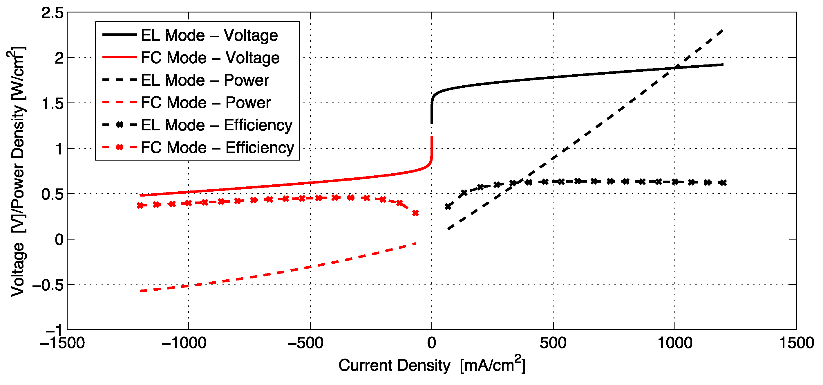
Finally, the RePEM performance curves obtained with the above exposed model, i.e., polarization curve, power and efficiency, are shown in Figure 4 as a function of the current density. In this plot, current is negative in FC mode and positive in EL mode. One can immediately note that the device performs better when it operates in EL mode than in FC mode, the latter one supplying a maximum power nearly 26% lower than the former one. Nonetheless, in the proposed power plant the excess power to be absorbed in EL mode is always significantly higher than the maximum power to be supplied in FC mode and, therefore, the performance curves are well suited for the application.
(4) Hydrogen tank: the hydrogen tank stores hydrogen produced by the RePEM in EL mode for later use by the RePEM itself in FC mode. The hydrogen tank is defined as the maximum amount of hydrogen it should contain in kilograms as shown in Table 1; the process of adding hydrogen to the tank is assumed to consume the electricity required by the compressor and the tank experiences no leakage. In this work, the initial tank level is set to the 5% of the maximum tank level and no constraints hold on the final tank level at the end of the year.
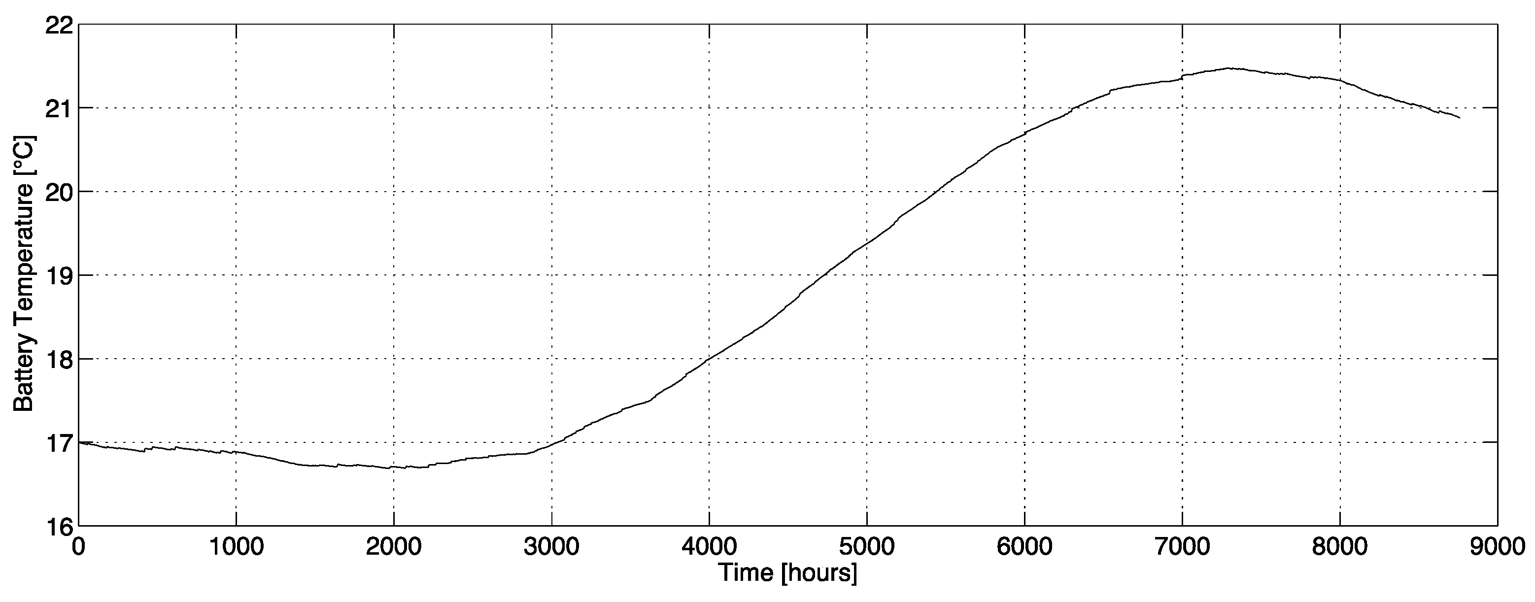
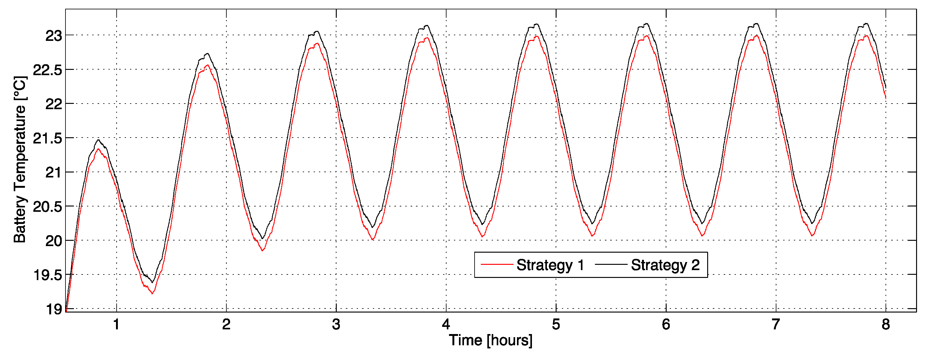
(5) Battery pack: the BAT has been modeled by means of a zero order equivalent circuit model. In this model, VOC,BAT is the open-circuit voltage, RBAT is the equivalent internal resistance and VBAT is the load voltage across the cell terminals. In this analysis, VOC,BAT and Qnom, which is the nominal charge capacity, are approximated as a function of SOC, while RBAT is mapped as function of both SOC and battery operating temperature, TBAT.
The battery operating temperature has been evaluated as the ambient temperature summed by a temperature variation related to internal thermal losses, which can be calculated from the current IBAT and the internal resistance as proposed by [25], according to:
T BAT ( t ) = T BAT ( t = 0 ) + o t R BAT I BAT 2 T BAT ( t ) T amb ( t ) R th C th d τ
which represents a first order differential equation, with parameters for thermal resistance Rth and thermal capacity Cth—a function of the specific BAT geometry, mass and materials. The term RBATIBAT2 represents the power loss in the battery and τ is the integration time variable.
Knowing the battery temperature and state of charge, VOC,BAT(SOC) and RBAT(SOC,TBAT) can be estimated and, for a flowing current, the battery voltage output can be derived from the well-known Kirchhoff voltage law:
V BAT = V OC , BAT ( SOC ) R BAT ( SOC , T BAT ) I BAT
By multiplying both sides by the current IBAT (positive during discharge), the battery power is expressed as:
P BAT = V BAT I BAT = V OC , BAT ( SOC ) I BAT R BAT ( SOC , T BAT ) I BAT 2
The variation of the battery SOC is proportional to the current at the battery terminal by means of the following:
S O ˙ C = I BAT Q nom
Hence, the SOC variation can be evaluated by solving Equation (14) for the current and expressing the state of charge derivative in Equation (15) as a function of battery power.
For the battery lifetime estimation, the semi-empirical algorithm proposed by [26] for OPzS (flooded lead acid type) batteries, which considers both the dependence on depth of discharge (DOD) and operating temperature, is employed. The applied algorithm estimates the maximum number of cycles NC, and thus the aging rate, as shown in the following:
N C ( DOD , T BAT ) = { 11.250 e 8.087 · DOD + 2836 e 1.17 · DOD if   0 < T BAT 20 ° C ( 11.250 e 8.087 · DOD + 2836 e 1.17 · DOD ) · ( 37.68 T BAT 1.101 0.3897 ) if   T BAT > 20 ° C
In the present study, the depth of discharge to be used in Equation (16) is evaluated as the moving average of the instantaneous DOD, calculated with a sample time of 1 h. The aging rate is the reciprocal of the number of cycles obtained with Equation (16), but an index of the battery lifetime is the cumulate of the aging rate of each cycle, which gives the aging rate corresponding to the total number of cycles experienced by the battery. When this index reaches the value of 1, the number of cycles equals the maximum number of cycles the battery can undergo and the battery is at the end of its life. Therefore, the reciprocal of the cumulated aging rate represents the battery lifetime, measured in years.
(6) Converter: the power converter is simply modeled as a device crossed by electrical power, affected by losses, PCONV,L, so that:
P CONV , L = P CONV , IN P CONV , OUT
For sake of simplicity, these losses have been considered to count for the 5% of the total net power flow across the converter.

3. Power Management Strategy

This section explains the control strategies proposed for the afore-described hybrid power plant. As already mentioned, a rule-based approach has been implemented for the plant power management strategies because of its reliability. PV and WT are used as primary generation sources to fulfill the required load demand, but—due to the intrinsic intermittency of renewable energy and its randomic nature in time, being not predictable in advance—a battery/RePEM/Diesel backup system is integrated to these renewable power converters to absorb excess power and satisfy possible unmet load.
In both the paradigms, battery is always used as primary backup system, followed by the fuel cell and then by the diesel generator when needed, while waste energy recovery is accomplished first by the battery and then by the RePEM in one case and vice versa in the second case. The two strategies are shown, respectively, in Figure 5 and Figure 6.
The backup diesel generator is included in the power plant to cope with failures and lack of energy storage.
The key difference between the two strategies is the excess energy recovery path. Since the final state of charge and hydrogen tank level are unconstrained at the end of the operation horizon, the comparison aims at evaluating the different plant performance in the two strategies. In particular, the plant performance is evaluated in terms of diesel fuel consumption (and CO2 emissions), battery aging rate and lifetime and energy consumed by the compressor. By considering all the energy flows in the hybrid power plant, an overall efficiency can be defined and compared between the strategies and the scenarios. Using a RePEM as primary energy recovery system—thus charging and discharging the hydrogen tank too often—implies a larger use of the hydrogen compressor, which could reduce the overall power plant efficiency and waste part of energy recovered. This effect is expected to increase with the RePEM and hydrogen tank sizes. On the other hand, using the battery as primary recovery energy system could accelerate its degradation by increasing the aging rate and reducing its lifetime.
In both cases, the hybrid polygeneration system must satisfy the following:
P Load = P WT + P PV + P RePEM + P BAT   + P ICE   P COMPR P CONV , L
where PWT is the power generated by the wind turbine, PPV is the power generated by the photovoltaic energy conversion system, PRePEM is the power generated by the reversible fuel cell (positive in FC Mode and negative in Electrolyzer Mode), PBAT is the battery power (positive in discharge and negative in charge), PICE is the backup diesel generator power, PCOMPR is the power required by the hydrogen compressor, and PCONV,L evaluates the power losses introduced by the converter. To evaluate the compressor power consumption, an optimized interrefrigerated compression has been considered and an isentropic compressor efficiency of 75% has been used.
Both the strategies are such that solar and wind technologies are always run at the maximum available power at the specific climatic conditions. If the renewable power, i.e., PRNW = PWT + PPV is greater than the load power PLoad (including converter losses and compressor power demand), the extra power is sent to the battery, if the battery state of charge is lower than 90%, otherwise the extra power is recovered by in the form of hydrogen, if the tank is not completely full. In this case, the excess power will be diverted to another dump load.
In Strategy 1, when the renewable power is lower than the required load, until there is hydrogen available in the tank, the fuel cell is used to satisfy the unmet power demand and the battery is by-passed. If there is no more hydrogen to be used, but SOC 30 % , the battery is used instead of the fuel cell for the unmet power demand. Finally, if both stored hydrogen and battery SOC are at their minimum levels, equal to 3 kg and 30% SOC, respectively, then the diesel backup generator must be switched on. Moreover, in this strategy, a sensitivity analysis has shown that the best results are obtained when the hydrogen tank is refilled up to 300 kg—which means completely refilled in Scenarios 1 and 2—before making the fuel cell available again.
In Strategy 2, when the renewable power is lower than the required load, if SOC 30 % , the battery is used to satisfy the unmet power demand and the fuel cell is by-passed. When SOC < 30 % , until hydrogen is available in the tank, the fuel cell is used to satisfy the unmet power demand. Again, if both stored hydrogen and battery SOC are at their minimum levels, equal to 3 kg and 30% SOC respectively, then the diesel backup generator must be switched on. Nevertheless, in this strategy, the fuel cell is available as soon as hydrogen is available in the tank.

4. Simulation Results

Results are proposed for the two strategies and the five scenarios listed in Table 1. The same electrical load profiles used in the components sizing phase and shown in Figure 2 have been used for the simulation of the power plant operation. Those profiles represent typical summer and winter daily loads and have been repeated to reproduce one-year and eight-year horizon loads. The hybrid plant operation has been simulated by means of an energy-based quasi-static simulator developed in Matlab/Simulink® environment [17].
A set of parameters has been chosen to compare the performance of the two strategies and namely: battery state of charge, hydrogen tank level, diesel fuel consumption, battery aging rate and lifetime, energy consumed by the compressor and power plant overall efficiency ηPP. This last parameter has been defined as the ratio between the power consumed by loads (end-users and hydrogen compressor) and converter inefficiencies and the power supplied by the renewable power sources and the diesel generator:
η PP =   P Load + P CONV , L + P COMPR P RNW + P ICE
It is clear that, in Equation (19), PLoad, PCONV,L and PRNW stay the same in the different scenarios, unlike PCOMPR and PICE.
Figure 7 and Figure 8 show the battery behavior in terms of SOC for Strategy 1 and 2, respectively, during the whole year for the different investigated scenarios. For Strategy 1 (Figure 7) it can be noted that the battery works in a different way for all the considered scenarios. In fact, in this strategy, when the renewable power is lower than the required load, until there is hydrogen available in the tank, the fuel cell is used to satisfy the unmet power demand and the battery is by-passed. Therefore, the battery SOC changes when the sizes of RePEM and hydrogen tank vary, respectively.
On the contrary, for Strategy 2 (Figure 8), as expected, the battery SOC is always the same for all the considered scenarios. In fact, in this strategy, when the renewable power is lower than the required load, if SOC ≥ 30%, the battery is used to satisfy the unmet power demand and the fuel cell is by-passed. Therefore, the battery SOC cannot change when the sizes of RePEM and hydrogen tank vary.
Figure 9 and Figure 10 show the hydrogen tank level for Strategy 1 and 2, respectively, during the whole year for the different investigated scenarios. For Strategy 1 (Figure 9) it can be noted that the RePEM works very often for all the considered scenarios. In fact, the hydrogen tank level in this strategy increases and decreases very frequently, so quickly that the tank is never completely filled. This is due to the fact that, in order to satisfy the unmet power demand, the fuel cell is used as primary system until the hydrogen is available, while the battery is used only as a backup system. Therefore, the RePEM is called to work many times in short periods.
On the contrary, in Strategy 2 (Figure 10), the hydrogen tank level profile is much smoother than in the first strategy and the variation trend is the same for all the considered scenarios; the only difference lies in the fact that is it scaled according to the capacity of the hydrogen tank. This is what should be expected in this strategy because, when the renewable power is lower than the required load, if SOC ≥ 30%, the battery is used as primary system to satisfy the unmet power demand and then the fuel cell is only employed as a backup system.
Table 2 for Strategy 1 and Table 3 for Strategy 2 provide a comparison of the performance parameters—i.e., diesel fuel consumption, battery aging rate and lifetime, compressor energy consumption and power plant overall efficiency—in the five scenarios. One can observe that Strategy 2 allows achieving better results in terms of fuel consumption for each scenario. Moreover, Table 3 underlines that the battery aging is not affected by the changes in the RePEM size, as in Strategy 2 the RePEM basically acts as a backup system and the battery is used in the same way in all the scenarios. On the contrary, in Strategy 1 the aging rate changes from one scenario to the other as the increase in the RePEM reduces the battery usage. Nonetheless, using the RePEM—thus charging and discharging the hydrogen tank—too often, implies a larger use of the compressor, reducing the overall power plant efficiency.
Scenario 2 results in being the best solution for both the strategies in terms of fuel consumption, overall efficiency and, for Strategy 1, also in terms of battery lifetime, but Strategy 2 allows achieving a fuel saving, over one year, greater than 47% despite increasing the battery aging rate and thus reducing its lifetime of only 1.8%.
Even if in Strategy 1 the RePEM is used as primary system in supplying power to fulfill unmet power demand, the diesel fuel consumption seems to be less affected by changes in the RePEM maximum power and capacity. This is probably due to the low efficiencies of the system when operating as fuel cell, which results in an ineffective management of the stored energy.
Table 4 shows the reversible PEM efficiencies in the five scenarios for the two strategies. One can note that the overall system efficiency is very similar for the same Scenario and different Strategy. This is mainly due to the efficiency of the system in EL mode, which is generally high and less affected by load variations, as one can observe in Figure 4. On the other hand, Scenarios 3 and 4 are characterized by a significant decrease of the efficiency in FC mode, as the FC is operated at a maximum power of 300 kW when the nominal power of the system is 1000 kW. Even if a fuel cell generally behaves better at partial loads, at very low loads the efficiency drops down because of the sudden increase of the activation overpotential. Nevertheless, even if the RePEM efficiency is somehow affected by the chosen strategy and worsen in the second Scenario, a better management of the stored energy allows reducing the need of the Diesel generator, thus decreasing the fossil fuel usage and increasing the power plant overall efficiency, Table 2 and Table 3.
Finally, Figure 11 and Figure 12 compare the energy storage for the best Scenario, i.e., Scenario 2, and the two strategies. Figure 11 compares the battery SOC for the best scenario (minimum fuel consumption), for Strategy 1 and 2, over the whole year. In Strategy 2, it can be noted how the battery is more deeply discharged. For example, after 5500 h, the SOC is equal to 55% for Strategy 1 and to 69% for the Strategy 2, while, at 3750 h, it is equal to 58% and 73% for Strategy 1 and 2, respectively. This is due to the fact that in these periods the fuel cell is turned off, therefore the battery is called to work to a greater extent to satisfy the unmet power demand. However, one can observe that the profile of the battery SOC is very similar in the two strategies during the rest of the year, and in very sporadic cases a slight misalignment of the two profiles exists. This helps understanding why the same Scenario results in being the best one for both the Strategies.
In Figure 12, the hydrogen tank level for the best scenario (minimum fuel consumption), for Strategy 1 and 2, is compared over the whole year. As said before, for Strategy 1, it can be noted how the tank level varies rapidly, as the RePEM is called to work many times in short periods. Counterwise for Strategy 2, the tank level has a smoother trend with long periods during which the RePEM produces or uses the hydrogen and long periods (2600–4100 h; 4800–5900 h) during which the level remains unchanged.
More interesting is the different value of the tank level at the end of the first year. In order to understand its influence on the second year of operation, results have also been evaluated for the same scenarios and strategies in an eight-year horizon simulation. This allows taking into account the effect of the unconstrained final tank level and battery state of charge. In particular, this is expected to be more significant for Strategy 2, as at the end of the year both the storage systems are unavailable. On the contrary, Figure 9 and Figure 10 show that at the end of the first year the final value of the tank level is quite high in all the scenarios, making the fuel cell available at the beginning of the following year, for Strategy 1. Moreover, this eight-year horizon simulation allows also taking into account the battery temperature increase and its effect on battery aging. Figure 13 shows that at the end of the first year the battery temperature is 3 °C greater than the initial temperature. Therefore, results can change significantly.
Table 5 and Table 6 compare the same parameters presented above, for the best scenario, i.e., Scenario 2, for the two strategies on this eight-year horizon. In particular, Table 5 shows the values obtained with an eight-year-long simulation, while Table 6 shows the annual averages obtained in a one-year-long simulation multiplied by eight, in order to obtain the eight-year horizon results. Interesting are the differences in the battery aging evaluation. In particular, running an eight-year-long simulation suggests that the battery would last almost one year less than the one-year simulation forecast. This is related to the battery temperature increase, not taken into account in the second case. Figure 14 portrays the battery temperature variation in the entire eight-year horizon, showing also that the trend tends to stabilize, with the maximum and minimum operating temperatures reaching a plateau.
Table 5 also underlines that with Strategy 1 the plant would most likely consume 110 kg of fossil fuel more than what obtained with the one-year simulation (Table 6), while in Strategy 2 the consumption increases of 370 kg, which nearly 13% more than the value retrieved with the one-year simulation. On the other hand, for the fuel cell the average efficiency obtained in the eight-year simulation is greater than the one obtained with the one-year simulation in both the strategies. This can be explained by looking at Figure 15a,b comparing the fuel cell power and tank level profiles for the first four months of the Year 1—i.e., the second year of power plant operation—evaluated in an eight-year horizon simulation and in a one-year horizon simulation. These figures show that, at the beginning of the Year 1 a hydrogen tank level different from zero allows using the fuel cell sooner than in the one-year simulation (which can be seen as a strategy with constrained final SOC and tank levels). This is particularly evident in Strategy 1, where the constraint of making the fuel cell available only when the fuel tank is completely refilled applies. In fact, in Strategy 2 (Figure 15b) the fuel cell operation is more similar. Still, in Figure 15c, one can note that also the initial value of state of charge lower than 90% has a great influence on the plant operation, as the electrolyzer is not used during the first days of the year and there is less hydrogen stored in the tank when the fuel cell is switched on. Nonetheless, with respect to the RePEM efficiencies, the error of considering a one-year simulation, instead of an eight-year one is less significant, due to the overall trend of the device operation, which is very similar. Analogous considerations hold for the electrolyzer.
By using the IPCC methodology [27], these two strategies can also be compared in terms of avoided CO2. This methodology defines the calculation of carbon dioxide emissions from the following equation:
C O 2 = C F · N C V · E F
where CF is the quantity of consumed fuel expressed in t/year, NCV net calorific value of fuel (TJ/tons), and EF is the emission factor (more precisely, kg CO2/TJ fuel). The coefficients utilized for this analysis are retrieved from [27] and are 45 GJ/tons for NCV and 73,300 kg CO2/TJ fuel for EF.
In Table 7 and Table 8, the CO2 avoided with respect to a baseline case—which considers the entire load satisfied by a diesel generator—is estimated for all the Scenarios and the two strategies. The baseline case presents a fuel consumption equal to 436 t/year, which corresponds to a production of CO2 equal to 1437 t/year.
The comparison of the two strategies with the baseline case shows that in the worst case a 96% reduction of CO2 emissions is achieved, reduction that reaches 98% for Scenario 2 in Strategy 2.
Therefore, the two strategies proposed for the management of the hybrid power plant, have in any case an environmental impact significantly lower than the diesel baseline case taken as reference.

5. Conclusions

In this paper, an off-grid hybrid wind/solar power plant with multiple storage technologies for an isolated system has been designed and two possible power management strategies for the stored energy have been compared. Wind and solar technologies have been used as primary power suppliers, while a lead-acid BAT and a reversible polymer electrolyte fuel cell have been employed to store the extra power, in order to fulfill the power demand when needed. The choice of a reversible PEM fuel cell has been made in order to reduce costs and occupied space. As in the proposed power plant the excess power to be stored is always significantly higher than the maximum power to be supplied in FC mode, the performance curves of the RePEM are well suited for the application. The different behavior of this device when operating in FC and EL modes has been investigated by varying the system maximum power and tank capacity proposing five different scenarios, and the influence of two possible control strategies of the stored energy has been analyzed for the proposed scenarios. Results have been compared in terms of fuel consumption and CO2 avoided, battery aging and power plant overall efficiency. Those parameters have also been used to evaluate the final RePEM size and energy management strategy.
Even if the plant aims at a 100% sustainable operation, none of the proposed Scenarios and Strategies is capable of completely avoiding the operation of the Diesel generator backup system. Nonetheless, in the worst case—i.e., RePEM is not included in the plant and the two strategies coincide, as only one energy storing device is considered—15.74 t/year of fossil fuel are consumed, which means 96% less CO2 emissions than a diesel-only-powered plant, taken as reference. The best situation, which consumes only 8.23 t/year of fossil fuel is the 300 kW RePEM, 100 kg hydrogen tank configuration, in which the battery is used as primary system both in storing energy and supplying extra power, while the RePEM is used as a backup system, before the Diesel generator operation. This case has an overall power plant efficiency equal to 84.49%, 0.4% higher than the same scenario managed with the other strategy thanks to the lower values of the energy consumed by the diesel generator and the hydrogen compressor. In fact, the fuel saving is higher than the 47% (8.23 t/years against 15.57 t/year), while the different management of the stored hydrogen allows reducing the compressor energy consumption of around 53%. In terms of battery aging, the battery lifetime is reduced by only 1.8% passing from 11.09 estimated years of lifespan to 10.89.
Results significantly change when they are compared in an eight-year horizon with respect to a one-year horizon. In particular, the effect of the lack of constraints on the tank level and battery state of charge at the end of the year on the performance parameters has been investigated. In particular, this effect is expected to be more significant for Strategy 2, as at the end of the first year both the storage systems are emptied. On the contrary, in Strategy 1, at the end of the first year the amount of the stored hydrogen is quite high in all scenarios, making the fuel cell available at the beginning of the following year. Moreover, in an eight-year horizon simulation, the battery temperature also increases and its effect on battery aging can be analyzed. Considering the best scenario (Scenario 3), results show an increase of fuel consumption estimation of 0.7% in Strategy 1 and of 5% in Strategy 2, which still consumes less fossil fuel. For the battery aging an underestimation of more than 7% and 8%, for Strategy 1 and 2, respectively, is observed with the one-year-long simulation, leading to a lifetime shortening of more than nine months in Strategy 1, and nearly 11 months in Strategy 2.
Nevertheless, both the Strategies allow achieving good results both in terms of fossil fuel consumption and battery aging and, in particular, the best compromise between fossil fuel usage and battery lifetime is represented by Strategy 2 and Scenario 3. Future studies will consider the possibility of including the RePEM aging estimation, which requires the validation of a specific semi-empirical aging model, similar to the one employed for the battery, by means of an experimental campaign.
Moreover, the inclusion of thermal load profiles could justify the application of an optimization algorithm aimed at minimizing the Diesel generator usage, while managing both electrical and thermal loads. Another interesting power management strategy to be analyzed is the one which employs battery and fuel cell in parallel, by making a controller decide which one should be used or if to use both of them. This control strategy could also be used to introduce in the optimization problem also the constraints on the state of charge and hydrogen tank level at the end of the year.

Author Contributions

Laura Tribioli realized the Matlab/Simulink simulator and designed the control strategy; Raffaello Cozzolino performed the power plant design optimization with HOMER; Laura Tribioli, Raffaello Cozzolino, Luca Evangelisti and Gino Bella performed the analyses and analyzed the data; and Laura Tribioli, Raffaello Cozzolino and Luca Evangelisti wrote the paper.

Conflicts of Interest

The authors declare no conflict of interest.

Nomenclature

AmRePEM cell active area (cm2)
APVPV area (m2)
ATWT swept area (m2)
BATBattery
CFConsumed fuel (t/year)
CpWT power coefficient (-)
DODBattery’s depth of discharge (%)
EFEmission factor (kg CO2/TJ fuel)
ELElectrolyzer
FFaraday constant (C/kmol)
FCFuel Cell
fPVPV scaling dimensionless factor
HOMERHybrid Optimization of Multiple Energy Resources
IBATBAT current (A)
ICEInternal Combustion Engine
INOCTPV nominal cell operating irradiance (kW/m2)
IRePEMRePEM input current (A)
ISIncident radiation on standard conditions (kW/m2)
ITIncident global solar radiation (kW/m2)
lmRePEM Membrane thickness (cm)
m ˙ H 2 RePEM hydrogen consumption or production mass flow rate (kg/s)
NCVNet Calorific Value (TJ/tons)
nsRePEM cell number
PBATBAT output power (kW)
PCOMPRCompressor power (kW)
PCONV,INConverter input power (kW)
PCONV,LConverter power losses (kW)
PCONV,OUTConverter output power (kW)
PICEICE generator power (kW)
PLoadLoad power demand (kW)
PPVPV output power (kW)
Prated,PVPV rated power (kW)
PRePEMRePEM power (kW)
PRNWRenewable power production (kW)
PVPhotovoltaic panel
PWTWT output power (kW)
QnomBAT Nominal capacity (Ah)
RBATBAT equivalent Resistance (Ohm)
RePEMReversible polymer electrolyte membrane fuel cell
RohmRePEM ohmic resistance (Ohm)
SOCBAT State of charge derivative (1/s)
SOCBattery’s state of charge (%)
TambAmbient temperature (°C)
TBATBAT operating temperature (°C)
TCPV cell temperature
TcellRePEM cell temperature (°C)
TNOCTPV nominal cell operating temperature (°C)
TrefPV reference temperature (°C)
TSPV standard reference temperature (°C)
VWind speed (m/s)
VBATBAT load voltage (V)
Vcut,inCut-in wind speed (m/s)
Vcut,offCut-off wind speed (m/s)
VOC,BATBAT open circuit voltage (V)
VOC,RePEMRePEM open circuit voltage (V)
VratedRated wind speed (m/s)
VRePEMRePEM input voltage (V)
WTWind Turbine
βPV array efficiency temperature coefficient (1/°C)
ηcBAT coulombic efficiency
ηFFaraday efficiency (-)
ηPVPV efficiency (-)
ηPV,refPV reference efficiency (-)
λmRePEM membrane hydration parameter (-)
ρAir density (kg/m3)

References

  1. Siviero, E. Mediterranean bridging and TUNeIT, the bridge between Tunisia and Italy. In Proceedings of the World Engineering Conference on Sustainable Infrastructure WECSI2014, Abuja, Nigeria, 2–7 November 2014.
  2. Chen, F.; Duic, N.; Manuel Alves, L.; da Graça Carvalho, M. Renew Islands—Renewable energy solutions for islands. Renew. Sustain. Energy Rev. 2007, 11, 1888–1902. [Google Scholar] [CrossRef]
  3. Mihalakakou, G.; Psiloglou, B.; Santamouris, M.; Nomidis, D. Application of renewable energy sources in the Greek islands of the South Aegean Sea. Renew. Energy 2002, 26, 1–19. [Google Scholar] [CrossRef]
  4. Lund, H.; Mathiesen, B.V. Energy system analysis of 100% renewable energy systems—The case of Denmark in years 2030 and 2050. Energy 2009, 34, 524–531. [Google Scholar] [CrossRef]
  5. Brown, P.D.; Pecas Lopes, J.A.; Matos, M.A. Optimization of pumped storage capacity in an isolated power system with large renewable penetration. IEEE Trans. Power Syst. 2008, 23, 523–531. [Google Scholar] [CrossRef]
  6. Yin, J.L.; Wang, D.Z.; Kim, Y.T.; Lee, Y.H. A hybrid energy storage system using pump compressed air and micro-hydro turbine. Renew. Energy 2014, 65, 117–122. [Google Scholar] [CrossRef]
  7. Ibrahim, H.; Younès, R.; Basbous, T.; Ilinca, A.; Dimitrova, M. Optimization of diesel engine performances for a hybrid wind–diesel system with compressed air energy storage. Energy 2011, 36, 3079–3091. [Google Scholar] [CrossRef]
  8. Giaouris, D.; Papadopoulos, A.I.; Ziogou, C.; Ipsakis, D.; Voutetakis, S.; Papadopoulou, S.; Seferlis, P.; Stergiopoulos, F.; Elmasides, C. Performance investigation of a hybrid renewable power generation and storage system using systemic power management models. Energy 2013, 61, 621–635. [Google Scholar] [CrossRef]
  9. Ibrahim, H.; Ilinca, A.; Perron, J. Energy storage systems—Characteristics and comparisons. Renew. Sustain. Energy Rev. 2008, 12, 1221–1250. [Google Scholar] [CrossRef]
  10. Sinha, S.; Chandel, S.S. Review of software tools for hybrid renewable energy systems. Renew. Sustain. Energy Rev. 2014, 32, 192–205. [Google Scholar] [CrossRef]
  11. National Operative Program FC SMART GEN (PON01_02864); Program Operativo Nazionale “Ricerca e Competitività” 2007–2013 (PON “R&C”): Italy, 2012.
  12. Cozzolino, R.; Tribioli, L.; Bella, G. Power management of a hybrid renewable system for artificial islands: A case study. Energy 2016, 106, 774–789. [Google Scholar] [CrossRef]
  13. NASA Surface meteorology and Solar Energy. Wind speed at 50 m above the surface of the earth for terrain similar to airports, monthly averaged values over 10-year period (July 1983–June 1993). Available online: https://eosweb.larc.nasa.gov/sse/global/text/10yr_wspd50m (accessed on 18 August 2016).
  14. NASA Surface meteorology and Solar Energy. Global horizontal radiation, monthly averaged values over 22-year period (July 1983–June 2005). Available online: https://eosweb.larc.nasa.gov/sse/global/text/global_radiation (accessed on 18 August 2016).
  15. NASA Surface meteorology and Solar Energy. Air temperature, monthly averaged values over 22-year period (July 1983–June 2005). Available online: https://eosweb.larc.nasa.gov/sse/global/text/22yr_T10M (accessed on 18 August 2016).
  16. Hoppecke 24 OPzS 3000 Battery String Datasheet. Available online: http://www.batteriehaus.de/images/stories/pdf/Sunlight/Sunlight_OPZS/2V_24_OPZS_3000.pdf (accessed on 19 July 2016).
  17. Matlab/Simulink®. Available online: http://it.mathworks.com/products/simulink/?requestedDomain=it.mathworks.com (accessed on 19 July 2016).
  18. UGE 1000H turbine. Available online: http://www.etcgreen.com/horizontal-axis-wind-turbine-1mw (accessed on 19 July 2016).
  19. Skoplaki, E.; Palyvos, J.A. On the temperature dependence of photovoltaic module electrical performance: A review of efficiency/power correlations. Sol. Energy 2009, 83, 614–624. [Google Scholar] [CrossRef]
  20. Muller, M. Measuring and modeling nominal operating cell temperature (NOCT): NREL test & evaluation. [Golden, Colo.]: National Renewable Energy Laboratory. 2010. Available online: http://www.nrel.gov/docs/fy10osti/49505.pdf (accessed on 19 July 2016). [Google Scholar]
  21. Faruk Selamet, Ö.; Becerikli, F.; Mat, M.D.; Kaplan, Y. Development and testing of a highly efficient proton exchange membrane (PEM) electrolyzer stack. Int. J. Hydrogen Energy 2011, 36, 11480–11487. [Google Scholar] [CrossRef]
  22. Husar, A.; Strahl, S.; Riera, J. Experimental characterization methodology for the identification of voltage losses of PEMFC: Applied to an open cathode stack. Int. J. Hydrogen Energy 2012, 37, 7309–7315. [Google Scholar] [CrossRef] [Green Version]
  23. Lebbal, M.E.; Lecœuche, S. Identification and monitoring of a PEM electrolyser based on dynamical modelling. Intern. J. Hydrogen Energy 2009, 34, 5992–5999. [Google Scholar] [CrossRef]
  24. Sarrias-Mena, R.; Fernàndez-Ramírez, L.M.; García-Vázquez, C.A.; Jurado, F. Electrolyzer models for hydrogen production from wind energy systems. Intern. J. Hydrogen Energy 2015, 40, 2927–2938. [Google Scholar] [CrossRef]
  25. Jackey, A.R. A simple, effective lead-acid battery modeling process for electrical system component selection. SAE Tech. Pap. 2007. [Google Scholar] [CrossRef]
  26. Layadi, T.M.; Champenois, G.; Mostefai, M.; Abbes, D. Lifetime estimation tool of lead–acid batteries for hybrid power sources design. Simul. Model. Pract. Theory 2015, 54, 36–48. [Google Scholar] [CrossRef]
  27. Gómez, D.R.; Watterson, J.D. Stationary combustion. Available online: http://www.ipcc-nggip.iges.or.jp/public/2006gl/pdf/2_Volume2/V2_2_Ch2_Stationary_Combustion.pdf (accessed on 19 July 2016).
Figure 1. Power plant schematic configuration.
Energies 09 00661 g001
Figure 2. Power demand—Seasonal profiles.
Energies 09 00661 g002
Figure 3. Wind turbine power curve and power coefficient [18].
Energies 09 00661 g003
Figure 4. RePEM performance curves.
Energies 09 00661 g004
Figure 5. Power management control strategy schematic (Strategy 1).
Energies 09 00661 g005
Figure 6. Power management control strategy schematic (Strategy 2).
Energies 09 00661 g006
Figure 7. Battery State of Charge variation over one year (Strategy 1).
Energies 09 00661 g007
Figure 8. Battery State of Charge variation over one year (Strategy 2).
Energies 09 00661 g008
Figure 9. Hydrogen tank level (Strategy 1).
Energies 09 00661 g009
Figure 10. Hydrogen tank level (Strategy 2).
Energies 09 00661 g010
Figure 11. Comparison of the SOC for the best scenario in 1 and 2.
Energies 09 00661 g011
Figure 12. Comparison of the tank level for the best scenario in Strategy 1 and 2.
Energies 09 00661 g012
Figure 13. Battery temperature variation during the year.
Energies 09 00661 g013
Figure 14. Battery temperature variation during the 8 years.
Energies 09 00661 g014
Figure 15. Fuel Cell Power and Tank Level comparison in one-year and eight-year simulation for: (a) Strategy 1; and (b) Strategy 2. Battery SOC in one-year and eight-year simulation for (c) Strategy 2.
Energies 09 00661 g015
Table 1. Reversible polymer electrolyte membrane fuel cell (RePEM) power and tank capacity in the different scenarios.
No. of ScenarioRePEM Rated Power (kW)Hydrogen Tank Size (kg)
Scenario 000
Scenario 1300300
Scenario 23001000
Scenario 31000300
Scenario 410001000
Table 2. Strategy 1—Performance Parameters comparison in the five scenarios.
No. of ScenarioDiesel ICE (Internal Combustion Engine) Fuel Consumption (t/year)Battery Cumulated Aging Rate (%)Battery Average Lifetime (years)Compressor Energy Consumption (MWh)Power Plant Efficiency (%)
Scenario 015.749.1810.89083.18
Scenario 115.579.0311.078.2183.17
Scenario 215.579.0211.0911.0484.09
Scenario 315.639.0611.0413.09879.76
Scenario 415.639.0511.0519.780.04
Table 3. Strategy 2—Performance Parameters comparison in the five scenarios.
No. of ScenarioDiesel ICE Fuel Consumption (t/year)Battery Cumulated Aging Rate (%)Battery Average Lifetime (years)Compressor Energy Consumption (MWh)Power Plant Efficiency (%)
Scenario 015.749.1810.89083.18
Scenario 110.759.1810.892.6784.01
Scenario 28.239.1810.895.1784.49
Scenario 313.099.1810.893.6383.72
Scenario 411.769.1810.897.8884.09
Table 4. RePEM average efficiency comparison in the two strategies for the four scenarios.
No. of ScenarioStrategy 1Strategy 2
RePEM Overall Efficiency (%)Efficiency FC Mode (%)Efficiency EL Mode (%)RePEM Overall Efficiency (%)Efficiency FC Mode (%)Efficiency EL Mode (%)
Scenario 151.3650.1752.5550.3647.4653.26
Scenario 251.4250.2452.6150.0746.9353.21
Scenario 340.0721.8658.2740.4421.6659.21
Scenario 439.5821.1558.0238.3717.9458.79
Table 5. Performance Parameters comparison (eight years, eight-year simulation, Scenario 2).
Performance ParameterStrategy 1Strategy 2
Diesel ICE Fuel Consumption (t/year)15.688.603
Battery Cumulated Aging Rate (%)77.879.86
Battery Average Lifetime (No of Cycles)19031850
Battery Average Lifetime (years)10.2810
Average FC mode efficiency (%)51.7247.43
Average EL mode efficiency (%)52.6153.18
RePEM Overall Efficiency (%)52.1750.31
Table 6. Performance Parameters comparison (eight years, one-year simulation, Scenario 2).
Performance ParameterStrategy 1Strategy 2
Diesel ICE Fuel Consumption (t/year)15.578.23
Battery Cumulated Aging Rate (%)72.1673.44
Battery Average Lifetime (No of Cycles)20351996
Battery Average Lifetime (%)11.0910.89
Average FC mode efficiency (%)50.2446.93
Average EL mode efficiency (%)52.6153.21
RePEM Overall Efficiency (%)51.4250.07
Table 7. Strategy 1—CO2 avoided.
No. of ScenarioDiesel ICE Fuel Consumption (t/year)CO2 Produced (t/year)CO2 Avoided (%)
Scenario 015.7451.9196.38
Scenario 115.5751.3596.42
Scenario 215.5751.3596.42
Scenario 315.6351.5596.41
Scenario 415.6351.5596.41
Table 8. Strategy 2—CO2 avoided.
No. of ScenarioDiesel ICE Fuel Consumption (t/year)CO2 Produced (t/year)CO2 Avoided (%)
Scenario 015.7451.9196.38
Scenario 110.7535.4597.53
Scenario 28.2327.1498.11
Scenario 313.0943.1796.99
Scenario 411.7638.7997.30

