Exploring Reduction Potential of Carbon Intensity Based on Back Propagation Neural Network and Scenario Analysis: A Case of Beijing, China

Abstract

Carbon emissions are the major cause of the global warming; therefore, the exploration of carbon emissions reduction potential is of great significance to reduce carbon emissions. This paper explores the potential of carbon intensity reduction in Beijing in 2020. Based on factors including economic growth, resident population growth, energy structure adjustment, industrial structure adjustment and technical progress, the paper sets 48 development scenarios during the years 2015–2020. Then, the back propagation (BP) neural network optimized by improved particle swarm optimization algorithm (IPSO) is used to calculate the carbon emissions and carbon intensity reduction potential under various scenarios for 2016 and 2020. Finally, the contribution of different factors to carbon intensity reduction is compared. The results indicate that Beijing could more than fulfill the 40%–45% reduction target for carbon intensity in 2020 in all of the scenarios. Furthermore, energy structure adjustment, industrial structure adjustment and technical progress can drive the decline in carbon intensity. However, the increase in the resident population hinders the decline in carbon intensity, and there is no clear relationship between economy and carbon intensity. On the basis of these findings, this paper puts forward relevant policy recommendations.

1. Introduction

With the accelerated melting of two polar glaciers and rising sea levels in recent decades, global warming has become a major concern of the international community. To reduce greenhouse gases emissions and curb further global climate warming has turned into the common challenge faced by human society in this century. As the harm caused by climate warming continues to emerge, as well as the deepening awareness of the international community, a binding “Paris Agreement” was adopted in 2015. Of all the greenhouse gases, CO₂ emissions from human activity contribute most of the warming effect, and it has become the focus of emission reduction. China overtook the United States as the world’s largest carbon emitters in 2007. As of 2013, China contributed 27.1% of the world’s total carbon emissions [1]. China is facing increasing international pressure in terms of carbon emissions. Some research results supported that there was an environmental Kuznets curve between economic development and carbon emissions in China. That is to say, with the development of the economy, China’s carbon emissions will increase first and then decrease; however, the inflection point of carbon emissions cannot be reached in a short time [2,3]. As awareness of environmental protection has constantly been enhanced and carbon emissions reduction is gradually seen as an opportunity to transform the mode of economic growth, the attitude of China towards carbon reduction is shifting from passive response to a positive response. In 2009, China promised that carbon intensity would be reduced by 40%–45% by 2020 based on the 2005 level. Moreover, this target has been embedded in the mid-and-long plan of national economic and social development as a rigid constraint index [4]. The overall reduction goal is set at the national level, but there are significant differences in resource endowment, stage of economic development and technical level in the provinces, so it is impossible to require all provinces to take 40%–45% as the target of emission reduction. Therefore, the emission reduction potential of the provinces should be fully taken into account in the allocation and formulation of carbon emissions reduction targets [5]. The energy of Beijing mainly relies on external input, which makes the energy security system vulnerable to external interference. In addition, as one of the most developed provinces in China, it has more capital and technology to achieve low-carbon development. Therefore, in this paper, carbon mitigation potential in Beijing is studied to provide reference for the policy departments and other provinces.

Carbon intensity has been extensively studied in recent years; however, study mainly focused on the influence factors of carbon intensity. Fan et al. [6] analyzed the influencing factors of the carbon intensity of China’s energy consumption from 1980 to 2003 using Divisia index decomposition method. They found that the reduction of energy intensity was of decisive significance for the carbon intensity reduction, and the proportion of coal in primary energy should be further cut in the future. Based on the panel data of 48 states in the United States, Davidsdottir and Fisher [7] studied the correlation between carbon intensity and economic development during 1980–2000. They concluded that there was a clear bi-directional relation between carbon intensity and economic development; that is to say, maintaining rapid economic growth and reducing carbon intensity can occur simultaneously. This conclusion was consistent with the empirical study on the influence factors of carbon intensity in China, namely economic development was conducive to the reduction of carbon intensity [8]. The empirical study also indicated that the decline in the proportion of secondary industries was conducive to lower the carbon intensity. Zhang et al. [9] explored the driving factors of carbon intensity of China’s 29 provinces from 1995 to 2012 employing the Logarithmic Mean Divisia Index (LMDI) method, and revealed that energy utilization technology progress and energy structure optimization were the two major driving forces for the decline of carbon intensity in the second and tertiary industries. In addition, Yi [10] adopted fixed-effect panel regressions to test the impacts of clean-energy policies on carbon emissions of electricity sector in the U.S. states, and found that supply-side energy policy was conducive to the reduction of carbon intensity and more aggressive policies on the demand side were needed to reduce total carbon emissions in the U.S. electricity sector. Compared with the analysis of the influencing factors of carbon intensity, only a few studies have been conducted to calculate carbon intensity reduction potential. These studies tend to focus on the national level, whereas there is less research on the calculation of carbon intensity reduction potential of provinces. Wang et al. [11] employed Markov chain model to predict China’s carbon intensity trend in 2011–2020, and then the contribution of optimizing energy structure on carbon intensity reduction was evaluated. Their finding showed that optimization of energy structure would promote the achievement of carbon intensity target under various scenarios. From the perspective of the development of thermal power, Liu et al. [12] predicted China’s carbon intensity by 2020, and demonstrated that China could not reach their carbon intensity reduction target according to the current development trends of thermal power. However, the total amount of carbon emissions were calculated by carbon emissions of thermal power, there is a certain error in prediction results. Aim to explore carbon intensity in the context of economic growth and energy structure adjustment, Zhu et al. [13] analyzed the quantitative relationship between economic growth and energy consumption using cointegration theory. Their finding suggested that China could achieve reduction targets by 2020 under different scenarios. Long et al. [14] estimated the reduction potential of carbon intensity of Jiangsu Province in 48 scenarios using improved Human Impact Population Affluence Technology (IPAT) model, and the results indicated that only the northern and southern parts of Jiangsu province would accomplish the 40%–45% reduction target for carbon intensity in 2020 in all scenarios. In light of the Chinese government’s latest estimates, the average annual economic growth rate is expected to be 6.5% in 2015–2020. However, most of the literature generally considered the average annual growth rate for the period to remain at about 7% in the calculation of carbon intensity reduction potential. This overly optimistic forecast will result in larger errors in the future scenario settings. Therefore, new literature is needed to compensate for this deficiency.

Carbon intensity is equal to the ratio of carbon dioxide emissions to GDP in a country or region during a certain period; therefore, the existing studies mainly focus on the prediction of carbon emissions. The prediction method of carbon emissions mainly comprises the scenario analysis method, the Stochastic Impacts by Regression on Population, Affluence and Technology (STIRPAT) method and time series prediction method. Hao et al. [15] employed scenario analysis method to predict the greenhouse gases emissions of China’s passenger vehicles during 2014–2020, and demonstrated that the current implementation of carbon mitigation and energy consumption policies played a positive role in preventing the growth of emissions. Taking population, per capita GDP, energy intensity and the level of urbanization as the influencing factors, Wang et al. [11] constructed the STRIPAT model to predict the carbon emissions of Minhang District in 2015. Their finding indicated that Minhang District would reach the minimum emission in this circumstance where per capita GDP maintained a high growth rate and energy intensity decreased at a high speed and population growth rate and urbanization rate remained moderate. With an improved mixed nonlinear grey prediction model, Wang et al. [16] predicted carbon intensity in Chinese provinces and various sectors of the economy in 2020, and allocated abatement tasks in various provinces and departments according to the principle of minimizing the cost of emission reduction.

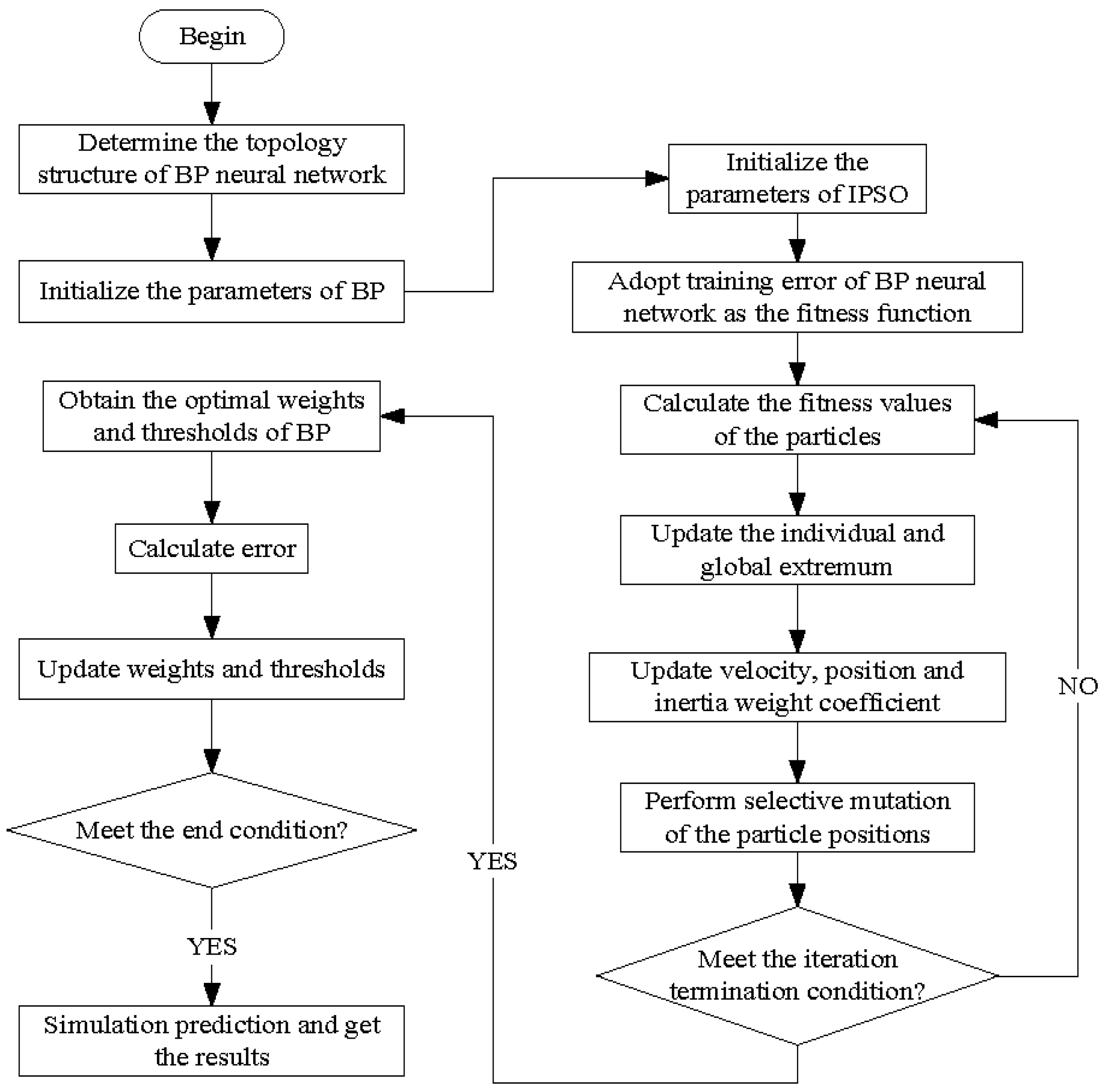
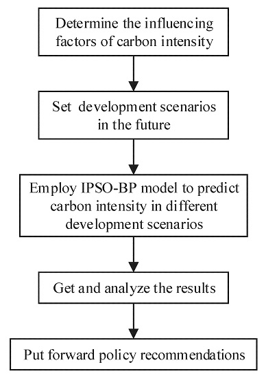
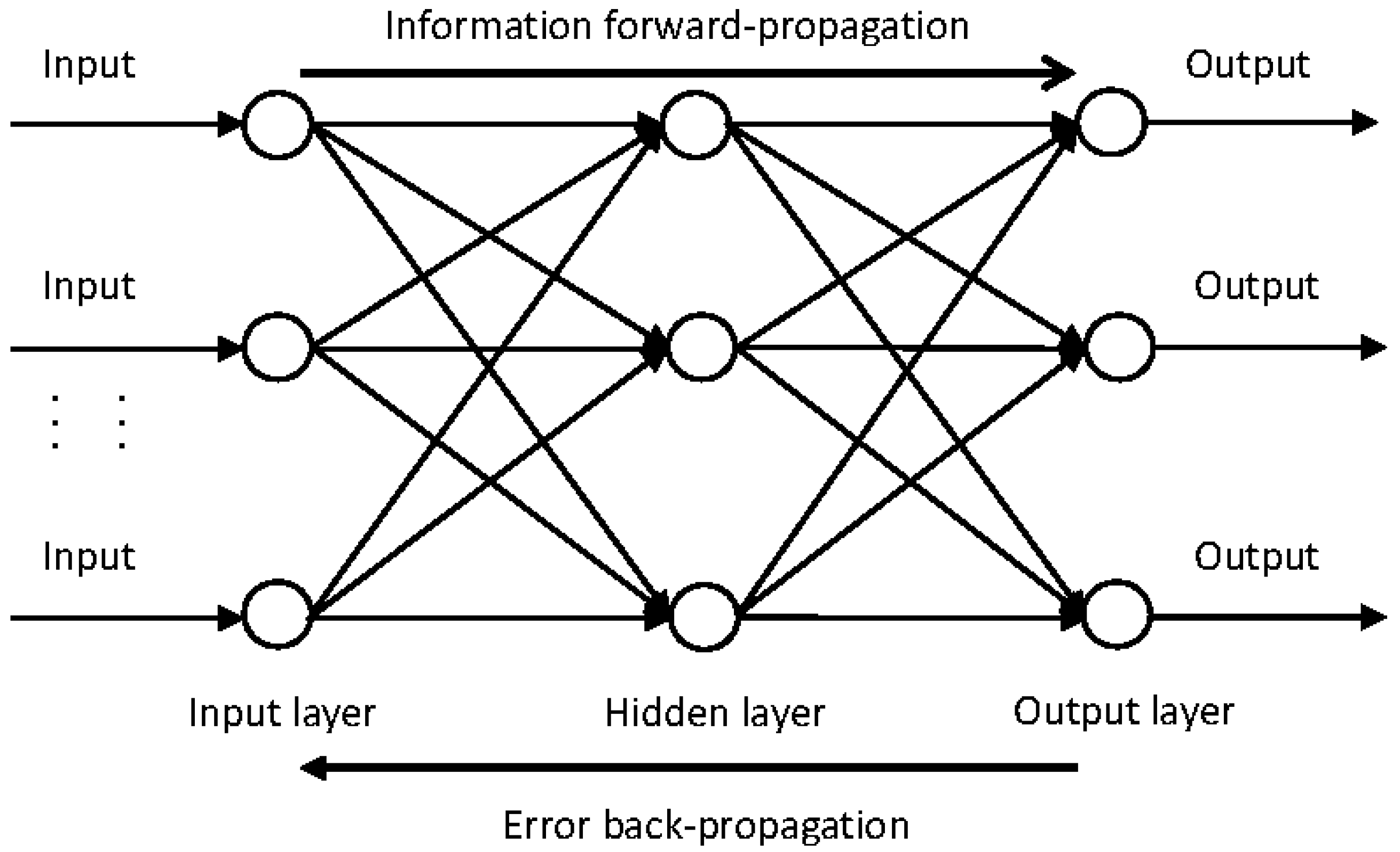
Scenario analysis is a kind of method to forecast probable events that can occur in the future. It can be used to compare the carbon emissions under different scenarios, however, large errors exist in the prediction results of the method. In the STIRPAT model, the effects of population, economy and technology on carbon emissions are taken into consideration. However, the prediction error caused by the multicollinearity of influencing factors cannot be avoided. Time series prediction method ignores the causal relationship between things and assumes that the development trend of things will continue in the future, therefore it only applies to the relatively short-term prediction. Aiming at the problems existing in the above methods, the back propagation (BP) neural network optimized by improved particle swarm optimization algorithm (IPSO) combined with scenario analysis method are proposed to forecast the carbon emissions and carbon intensity in Beijing in this paper. Because of the favorable self-organization and nonlinear mapping ability, BP neural network is suitable to predict carbon emissions of nonlinear systems affected by many factors. In order to enhance the global search ability and convergence ability of BP neural networks, IPSO is introduced to optimize the initial connection weights and thresholds of BP neural network, hereafter referred to as IPSO-BP. The IPSO-BP model not only makes full use of the global search ability of IPSO and local optimization capability of BP neural network, but also overcomes the intrinsic defects of BP neural network. In order to present the details of the measurement of carbon emissions reduction potential in Beijing, the rest of this paper will be deployed as follows. Firstly, based on the analysis of the influence factors of carbon emissions in Beijing using the grey relational analysis method (GRA), this paper takes GDP, resident population size, energy structure, industrial structure, technical level as the indicators to set the development scenarios of Beijing in the years 2015–2020. Secondly, the IPSO-BP model is adopted to calculate the carbon intensity reduction potential under different development scenarios. Finally, according to the results of the calculation, the policy recommendations are provided to exploit the potential of carbon emissions reduction in Beijing.

2. Material and Methods

2.1. Data Sources and Usage

The sources of the statistical data used in this paper included the China Statistical Yearbook [17], China Energy Statistical Yearbook [18] and Beijing statistical yearbook [19]. In order to exclude the impact of price factors, the final value of GDP and energy intensity were calculated based on the constant price of 2005, which is the base year.

2.2. Calculation of Carbon Intensity

There are no official carbon emissions and carbon intensity data that can be directly acquired, therefore the relevant data must be calculated in this paper. Carbon intensity is the ratio of carbon emissions to GDP. Given that the energy consumption of all varieties can be obtained from the statistical yearbook, carbon emissions are calculated according to energy balance sheet. To ensure the comparability of measurement results, carbon emission coefficients of various types of energy adopt the recommended value of IPCC [20]. Therefore, the total carbon emissions can be calculated as follows:

$$C={\displaystyle \sum _i^n{C}_i}={\displaystyle \sum _{i=1}^n{E}_i\times S_i\times F_i}$$

(1)

where C is the total carbon emissions, i refers to energy types, and C_i is the carbon emissions of energy i. E_i is the consumption of energy i, S_i is the conversion coefficient of energy i to standard coal, and F_i is the carbon emissions coefficient of energy i. It is assumed that the oxidation rate of various energy sources is 100%.

According to Equation (1), the amount of carbon emissions and carbon intensity are shown in Figure 1.

2.3. Grey Relational Analysis

Because there is a complicated non-linear relationship among numerous influencing factors of carbon emissions, it is impossible to take all the factors into account in the prediction of carbon emissions. According to the existing research results and the actual situation of carbon emissions in Beijing, this paper selects GDP, resident population, the energy structure, industrial structure, and technological level as the main factors of carbon emissions [21,22,23]. Coal accounted for the proportion of total primary energy consumption represents energy consumption structure; the industrial structure is represented by the tertiary industry output value accounted for the proportion of GDP; and the technical level is expressed by energy intensity. Then, the relationship between the five factors and carbon emissions is analyzed using the grey relational analysis method.

The grey relational analysis (GRA) is a kind of multi factor statistical method to quantitatively analyze and compare the development trend of a system [24]. It can be used to obtain the grey correlation degree between reference sequence and comparison sequence through the comparison of geometric similarity of time series data in the system [25]. The greater the grey correlation degree between the reference sequence and the comparison sequence is, the closer they are. GRA is often used to handle the relationship between objects with fewer data and unclear internal relations. The carbon emissions are selected as the reference sequence. The comparison sequences are GDP, the resident population, the energy structure, the industrial structure and the technical level. The grey correlation degrees between them are calculated by GRA. First of all, the non-dimensional treatment of the reference sequence and the comparison sequences are carried out, and then the correlation coefficients between the comparison sequence and the reference sequence are calculated, and finally the grey correlation degrees between them are obtained. The correlation degrees between the reference sequence and the comparison sequences are as follows:

$$r_{01}=0.7581; r_{02}=0.9576; r_{03}=0.8007; r_{04}=0.9473; r_{05}=0.7745$$

where r₀₁ represents the correlation degree between carbon emissions and GDP, r₀₂ represents the correlation degree between carbon emissions and the resident population, r₀₃ represents the correlation degree between carbon emissions and energy structure, r₀₄ represents the correlation degree between carbon emissions and industrial structure, and r₀₅ represents the correlation degree between carbon emissions and technical level.

The correlation degrees between the selected influencing factors and carbon emissions are all above critical value of 0.6, it can be considered that there is significant correlation between influencing factors and carbon emissions [26]. From the perspective of relevance, the effects on carbon emissions from strong to weak are the industrial structure, the resident population, the industrial structure, the energy structure, the technical level and GDP. As for as the correlation degrees between the influencing factors are concerned, the correlation degrees between the resident population and the industrial structure are the largest, and its value is 0.58. The correlation degrees between other influencing factors are below the critical value of 0.5; it can be considered that there are weak correlations between influencing factors. Therefore, these influencing factors are suitable to be used as explanatory variables to predict carbon emissions.

2.4. BP Neural Network Model

A back propagation (BP) neural network is a kind of multilayer feed-forward network with information forward propagation and error back propagation, which was proposed by research group led by Rumelhart and McCelland in 1986 [27]. In the process of training, the input signals are propagated from the input layer to the output layer via hidden layer, the neuron state of each layer is only affected by the neuron state of the upper layer. If there is an error between the output layer output and the desired output, the network is in the state of back propagation. In the process of back propagation, the gradient descent algorithm is used to adjust the weights and thresholds of the neural network layer by layer [28]. Through continuously correcting the weights and thresholds of the neural network in the back propagation, the accuracy of the neural network is improved. The topology of BP neural network is shown in Figure 2.

Although the BP neural networks can approximate any nonlinear function at arbitrary precision, it is easily trapped in the local optimization because of its nature of gradient descent method [29]. In addition, the initial parameters (weights and thresholds) of BP neural network are set randomly; therefore, the neural network convergence speed and the precision of the model are limited. To a certain extent, the parameters of BP neural network can be optimized by the expansion of training samples capacity. However, it also brings about the increase of time complexity and the phenomena of over-fitting, thus affecting the prediction accuracy. In order to improve the prediction accuracy and reduce the time complexity of the network, IPSO is adopted to optimize the initial connection weights and thresholds of BP neural network in this paper.

2.5. IPSO Algorithm

Particle swarm optimization algorithm (PSO) is an efficient swarm intelligence optimization algorithm proposed by Kennedy and Eberhart in 1995 [30,31], inspired by foraging process of bird flocking in nature. Each particle of PSO represents a potential solution to the problem, and there is a correspondence between particle and the fitness decided by fitness function. The direction and distance of the particle move are determined by the velocity of the particles, and the velocity is adjusted dynamically according to the moving experience of particle itself and other particles, thereby finding the optimal solution of the individual in the solution space.

Now suppose that there are $n$ particles in a D-dimensional search space. Population is represented by a particle collection X = (X₁, X₂, …, X_n), which represents all feasible solutions of optimization problems in the search space. The position of particle X_i is represented by a D-dimensional vector $X_i={\left[x_{i1},x_{i2},\cdots ,x_{iD}\right]}^T$. The vector is composed of a set of initial parameters of the BP neural network. The position of the particle is brought into the neural network as the weights and thresholds to get the prediction output, and the fitness value of the particle is the absolute value of the error between the predicted output and the desired output. The velocity of the particle X_i is represented by a D-dimensional vector $V_i={\left[V_{i1},V_{i2},\cdots ,V_{iD}\right]}^T$. The vector determines the search capability of each particle in search space. The optimal position that the ith particle has reached so far is $P_i={\left[P_{i1},P_{i2},\cdots ,P_{iD}\right]}^T$ and the corresponding fitness value is $Pbes{t}_i$, called an individual extremum. Likewise, the best position of the population has reached so far is $P_g={\left[P_{g1},P_{g2},\cdots ,P_{gD}\right]}^T$ and the corresponding fitness value is $Gbest$, called the global extremum. The particles update the velocity and position of the particles through the individual extremum and the global extremum in every iteration process. The update formula is as follows:

$$V_{id}^{k+1}=w{V}_{id}^k+c_1{r}_1(P_{id}^k-X_{id}^k)+c_2{r}_2\left(P_{gd}^k-X_{id}^k\right)$$

(2)

$$X_{id}^{k+1}=X_{id}^k+V_{id}^{k+1}$$

(3)

where w is the inertia weight coefficient, d (=1, 2, 3…D) refers to the dth dimensional space, i (1, 2, 3…n) refers to the ith particle, and k is the current iteration number. Moreover c₁ and c₂ are learning factors, and c₁ = c₂ = 1.49445, while r₁ and r₂ are random numbers distributed in [0, 1].

The PSO has fast convergence speed, but it still has the defects of easy premature and low later iteration efficiency. Therefore, the selective mutation operation inspired by the mutation idea of genetic algorithm is introduced in PSO to cope with the above shortcomings [32]. By means of reinitialization of the position variables of particles in the light of the preset probability, the selective mutation operation can make the particles jump out of the local optimum and search the optimal solution in a larger space. As a result of the selective mutation operation, the diversity of PSO population is increased, the search space of the population in the iteration process is widened, and the defects of easy premature and inefficiency in later iteration are improved. Moreover, variable inertia weight is applied to PSO to balance global and local search capabilities of particles [33]. Variable inertia weight can make PSO have larger inertia weight in the initial stage of iterations to maintain strong global search ability, and have smaller inertia weight in the later stage of iterations to enhance local search capability [34]. The formula of variable inertia weight is expressed as follows:

$$w\left(k\right)=w_{start}+\left(w_{start}-w_{end}\right)\left(2k/T_{\max }-{\left(k/T_{\max }\right)}^2\right)$$

(4)

where $w_{start}$ is the initial inertia weight, equal to 0.9; $w_{end}$ is the inertia weight in the latest stage of iterations, equal to 0.4; k is the current iteration number; and T_max is the maximum number of iterations.

2.6. IPSO-BP Model

In this paper, the BP neural network adopts three-layers structure. There are five input layer nodes in the BP neural network, corresponding to influencing factors of GDP, the resident population, the energy structure, the industrial structure and the technical level. There is one output node, corresponding to carbon emissions. According to the comparison of test results, the BP neural network can achieve the highest prediction accuracy with eight nodes in hidden layer. The maximal algebra of network iteration is 100 times, the error precision is set to 0.0001, and the learning rate is set to 0.1. In the IPSO algorithm, the number of population is 40, the maximal algebra of iteration is 80 times, and the mutation probability is set to be 0.9; moreover, the range of search space is [−5, 5], and velocity range is [−1, 1]. To enhance the representation of training samples, 15 of the 20 samples composed of related data during 1995–2014 are selected randomly as training samples, and the rest are regarded as test samples. The average test error of IPSO-BP neural network is 2.71%, and it is appropriate to predict the future carbon intensity in Beijing. The flow chart of the IPSO-BP algorithm is shown in Figure 3.

3. Description of Scenarios

According to the results of grey relational analysis, this study set scenarios for economic growth, resident population growth, energy structure adjustment, industrial structure adjustment, and technical progress based on different economic growth rates, resident population growth rates, energy structure adjustment rates, industrial structure adjustment rates and technical progress rates. Based on diverse economic growth rate, this study set three series: a low economic growth rate, a medium economic growth rate, and a high economic growth. Moreover, this study set medium and low rates of resident population growth, high and medium rates of energy structure adjustment, medium and low rates of industrial structure adjustment, and medium and low rates of technical progress. The details of scenario settings are described as follows.

3.1. Economic Growth

With economic expansion having moderated to a “new normal” pace, economic growth of Beijing showed a downward trend year by year during the Twelfth Five-Year Plan, and economic growth is expected to continue to decline in the future [35]. However, because of the driving effect of innovation to economic growth and the implementation of Beijing-Tianjin-Hebei regional integration and The Belt and Road Initiative, Beijing still has the potential to maintain medium-to-high growth of economy. In the government work report of 2016, the GDP annual average growth rate for Beijing was set at 6.5% in the Thirteenth Five-Year Plan [36]. Taking into account the actual situation of economic development and the economic plan of the government, the economic growth rate of Beijing is set to high, medium and low categories from 2015 to 2020 (

Table 1. Values set for economic growth rates of Beijing from 2015 to 2020 (%).

Year	High Growth Rate	Medium Growth Rate	Low Growth Rate
2015–2020	6.8	6.5	6.2

).

3.2. Resident Population Growth

In light of the statistical yearbook of Beijing, the average annual growth rate of the resident population in Beijing was 2% during the Twelfth Five-Year Plan, and the rate decreased year by year. Moreover, the government announced that the number of resident population would be controlled within 23 million during the Thirteenth Five-Year Plan. However, due to the obvious location advantages and resource advantages, the future population of Beijing will continue to maintain a rigid growth. Therefore, the population growth rate in Beijing is set to the medium and low categories from 2015 to 2020 (

Table 2. Values set for population growth rates of Beijing from 2015 to 2020 (%).

Year	Medium Growth Rate	Low Growth Rate
2015–2020	1.6	1.0

).

3.3. Energy Structure

According to the statistical yearbook of Beijing, coal consumption of Beijing accounted for the proportion of total primary energy consumption is 18.16% in 2014, and the ratio decreased by 66.63% compared to 1995. Because coal not only has a higher carbon emission coefficient but also causes haze easily, the government of Beijing plans to control the amount of coal consumption below nine million tons in 2020. Furthermore, the government of Beijing plans to make the total amount of energy consumption less than 88 million tons of standard coal in 2020 and make the proportion of high-quality energy increased to about 92% [37]. Therefore, the energy structure adjustment rate in Beijing is set to the high and medium categories from 2015 to 2020 (

Table 3. Values set for energy structure adjustment rates of Beijing from 2015 to 2020 (%).

Year	High Adjustment Rate	Medium Adjustment Rate
2015–2020	−10	−6

).

3.4. Industrial Structure

The tertiary industry output value of Beijing accounted for 77.9% of the GDP by 2014. With the promotion of Beijing-Tianjin-Hebei regional integration, the government more actively promotes the transition from industrial economy to the service economy and transfer of the secondary industry to the surrounding areas. Therefore, this study expects the proportion of tertiary industry will continue to ascend. Given the proportion of tertiary industry is already at the high level, its future growth will gradually slow down. Therefore, the industrial structure adjustment rate in Beijing is set to the medium and low categories from 2015 to 2020 (

Table 4. Values set for industrial structure change rates of Beijing from 2015 to 2020 (%).

Year	Medium Optimization Rate	Low Optimization Rate
2015–2020	0.8	0.5

).

3.5. Technical Progress

Beijing achieved an average annual economic growth of 8.6% in context of an average annual energy consumption growth of 2.5% from 2008 to 2014. The energy intensity fell by 23.66% during the Twelfth Five-Year Plan, which exceeded the energy intensity reduction targets of 17%. The energy intensity reduction target is set to 15% by government during the Thirteenth Five-Year Plan. Moreover, with the upgrade of the industrial structure, the optimization of energy structure and growing pressure on energy-saving and emission reduction, energy intensity will continue to decline in the future. Therefore, the technical progress rate in Beijing is set to the medium and low categories from 2015 to 2020 (

Table 5. Values set for technical progress rates of Beijing from 2015 to 2020 (%).

Year	Medium Optimization Rate	Low Optimization Rate
2015–2020	4.1	3.2

).

As shown in

Table 6. Set scenarios.

Combination of Index Change Rate
Base Development Scenario						Optimized Development Scenario						Strengthened Development Scenario
SS	EG	PG	ES	IS	TP	SS	EG	PG	ES	IS	TP	SS	EG	PG	ES	IS	TP
BD1	Low	Medium	Medium	Low	Low	OD1	Medium	Medium	Medium	Low	Low	SD1	High	Medium	Medium	Low	Low
BD2	Low	Medium	Medium	Low	Medium	OD2	Medium	Medium	Medium	Low	Medium	SD2	High	Medium	Medium	Low	Medium
BD3	Low	Medium	Medium	Medium	Low	OD3	Medium	Medium	Medium	Medium	Low	SD3	High	Medium	Medium	Medium	Low
BD4	Low	Medium	Medium	Medium	Medium	OD4	Medium	Medium	Medium	Medium	Medium	SD4	High	Medium	Medium	Medium	Medium
BD5	Low	Medium	High	Low	Low	OD5	Medium	Medium	High	Low	Low	SD5	High	Medium	High	Low	Low
BD6	Low	Medium	High	Low	Medium	OD6	Medium	Medium	High	Low	Medium	SD6	High	Medium	High	Low	Medium
BD7	Low	Medium	High	Medium	Low	OD7	Medium	Medium	High	Medium	Low	SD7	High	Medium	High	Medium	Low
BD8	Low	Medium	High	Medium	Medium	OD8	Medium	Medium	High	Medium	Medium	SD8	High	Medium	High	Medium	Medium
BD9	Low	Low	Medium	Low	Low	OD9	Medium	Low	Medium	Low	Low	SD9	High	Low	Medium	Low	Low
BD10	Low	Low	Medium	Low	Medium	OD10	Medium	Low	Medium	Low	Medium	SD10	High	Low	Medium	Low	Medium
BD11	Low	Low	Medium	Medium	Low	OD11	Medium	Low	Medium	Medium	Low	SD11	High	Low	Medium	Medium	Low
BD12	Low	Low	Medium	Medium	Medium	OD12	Medium	Low	Medium	Medium	Medium	SD12	High	Low	Medium	Medium	Medium
BD13	Low	Low	High	Low	Low	OD13	Medium	Low	High	Low	Low	SD13	High	Low	High	Low	Low
BD14	Low	Low	High	Low	Medium	OD14	Medium	Low	High	Low	Medium	SD14	High	Low	High	Low	Medium
BD15	Low	Low	High	Medium	Low	OD15	Medium	Low	High	Medium	Low	SD15	High	Low	High	Medium	Low
BD16	Low	Low	High	Medium	Medium	OD16	Medium	Low	High	Medium	Medium	SD16	High	Low	High	Medium	Medium

Note: SS represents scenario sequence, EG represents economic growth rate, PG represents resident population growth rate, ES represents energy structure adjustment rate, IS represents industrial structure adjustment rate, and TP represents technical progress rate.

, based on the varying economic growth rates, this study sets three main scenarios for Beijing: the base development scenario (BD), the optimized development scenario (OD), and the strengthened development scenario (SD). By combining the three main scenarios with each change rate of the five indexes set out above, 48 series are contained in this paper.

4. Results and Discussion

The combination of scenarios was taken as the predictive inputs of the IPSO-BP neural network to forecast carbon emissions in different scenarios in Beijing, and then the carbon emissions were divided by the corresponding GDP to get the carbon intensity. The carbon intensity of Beijing in different scenarios was as follows.

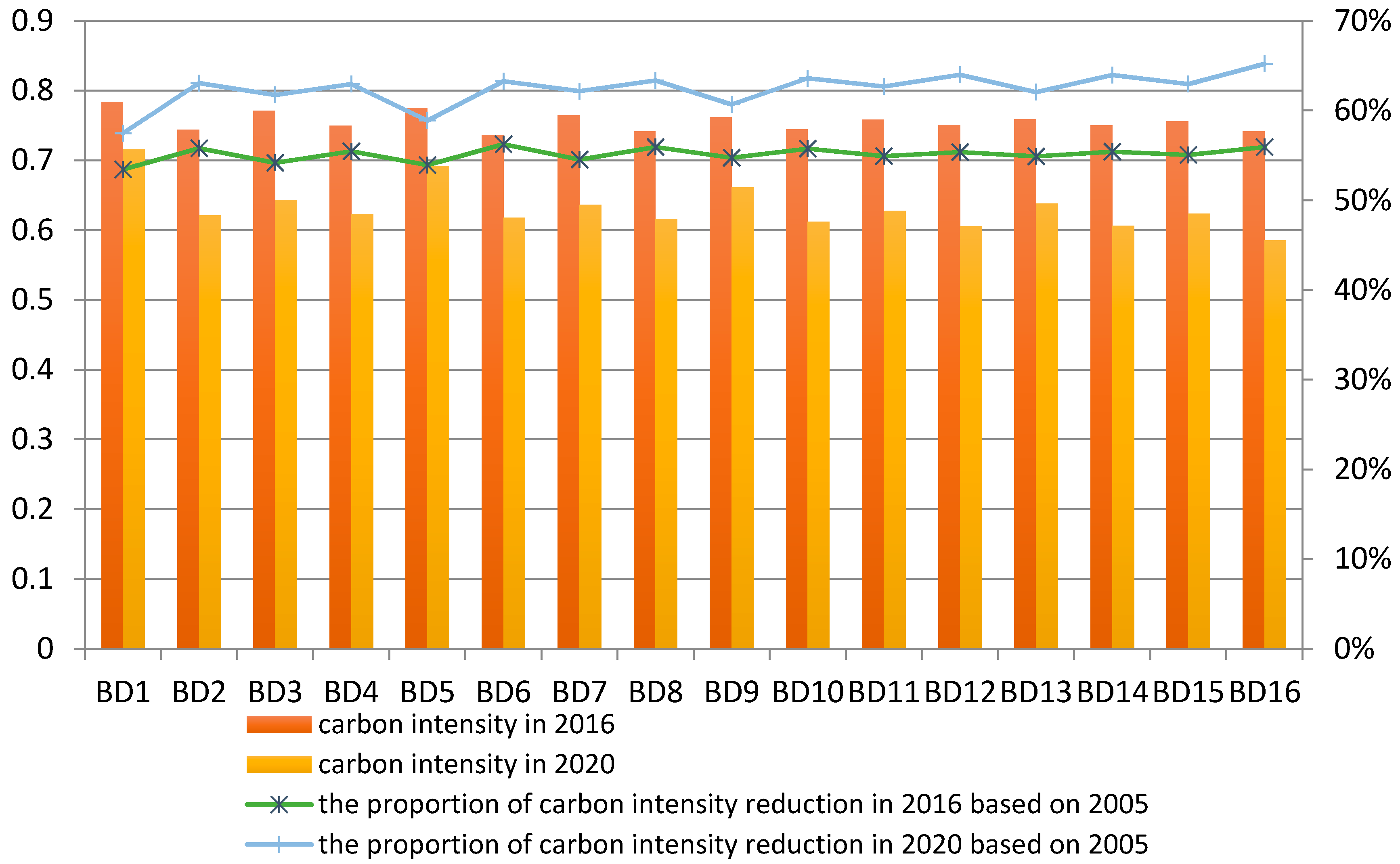
4.1. Calculation of Carbon Intensity in Based Development Scenarios

The base development scenarios comprised 16 kinds of series, and the economic development of these series was set at the low rate. The predicted values of carbon intensity and the proportion of carbon intensity reduction of Beijing in 2016 and 2020 are shown in Figure 4.

The prediction results revealed that the potential of carbon intensity reduction was above 53% in 2016 and above 55% in 2020 in the based development scenarios. The potential of carbon intensity reduction can exceed the 40%–45% reduction target of carbon intensity in 2020 in all series. For the prediction values of 2016 and 2020, carbon intensity would reach the peak in scenarios BD1, and the potential of carbon intensity reduction would achieve the minimum value in scenarios BD1, in which the resident population growth rate was at the medium level and the change rate of energy structure, industrial structure and technical progress were at the low level. In addition, carbon intensity would reach the minimum value in scenarios BD16, and the potential of carbon intensity reduction would be at the peak in scenarios BD16, in which the resident population growth rate was at the low level and the change rate of energy structure, industrial structure and technical progress were at the high level, medium level and medium level, respectively. The prediction results showed that the lower population growth rate, the higher energy structure adjustment rate, the higher industrial structure adjustment rate and the higher technical progress rate were conducive to the decline of carbon intensity, but the contribution of these influencing factors to carbon intensity was different. Through the comparison of BD2 and BD3, BD6 and BD7, BD11 and BD10, BD15 and BD14, the contribution of technical progress on carbon intensity reduction was 2.2 times higher than that of industrial structure adjustment. Through the comparison of BD3 and BD5, and BD11 and BD13, the contribution of energy structure adjustment on the carbon intensity reduction was 21% higher than that of the industrial structure adjustment. Although the rate of energy structure adjustment was greater than that of technical progress, the comparison of BD1 and BD6, and BD9 and BD14 showed that the contribution of technical progress on carbon intensity reduction was 1.4 times higher than that of energy structure adjustment. The growth of resident population went against the reduction of carbon intensity, the comparison of BD1 and BD9 indicated that if the resident population growth rate increased by 0.1%, the carbon intensity in 2020 would increase by 0.8%.

4.2. Calculation of Carbon Intensity in Optimized Development Scenarios

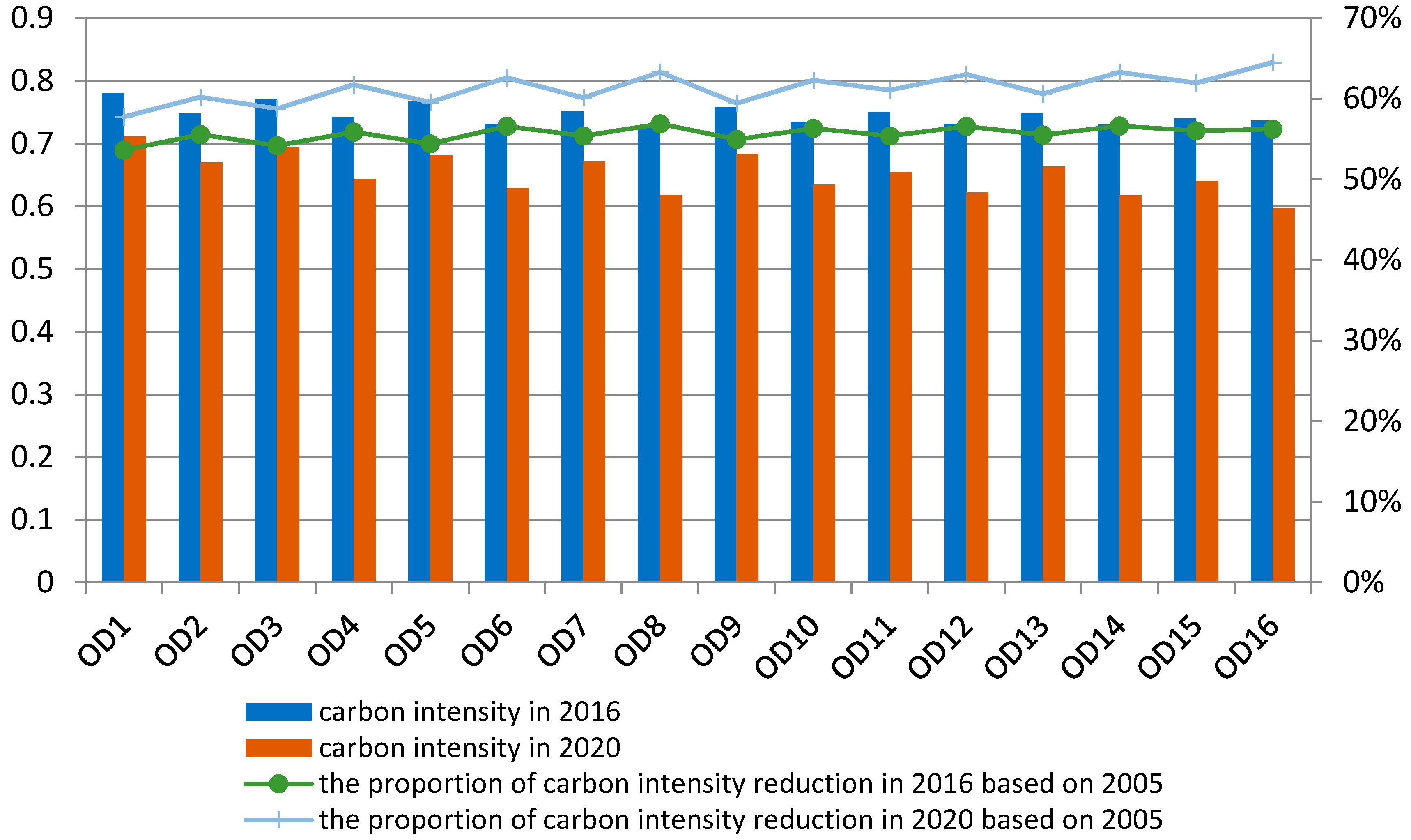
The optimized development scenarios contained 16 kinds of series, and the economic development of these series was set at the medium rate. The predicted values of carbon intensity and the proportion of carbon intensity reduction of Beijing in 2016 and 2020 are shown in Figure 5.

The prediction results indicated that the potential of carbon intensity reduction was above 53% in 2016 and above 57% in 2020 in the optimized development scenarios. The potential of carbon intensity reduction can exceed the reduction target of China in 2020 in 16 kinds of series. For the prediction values of 2016 and 2020, carbon intensity would reach the peak in scenarios OD1, and the potential of carbon intensity reduction would achieve the minimum value in scenarios OD1, in which the resident population growth rate was at the medium level and the change rate of energy structure, industrial structure and technical progress were at the low level. Furthermore, carbon intensity would reach the minimum value in scenarios OD16, and the potential of carbon intensity reduction would reach the peak in scenarios BD16, in which the resident population growth rate was at the low level and the change rate of energy structure, industrial structure and technical progress were at the high level, medium level and medium level respectively. Although the forecast results showed that the lower population growth rate, the higher energy structure adjustment rate, the higher industrial structure adjustment rate as well as the higher technical progress rate were conducive to the decline of carbon intensity, the contribution of these influencing factors to carbon intensity was different. Through the comparison of OD2 and OD3, OD6 and OD7, OD11 and OD10, and OD15 and OD14, the contribution of technical progress on carbon intensity reduction was 2.1 times higher than that of industrial structure adjustment. Through the comparison of OD3 and OD5, and OD11 and OD13, the contribution of energy structure adjustment on the carbon intensity reduction was 23% higher than that of the industrial structure adjustment. Although the rate of energy structure adjustment was greater than that of technical progress, the comparison of OD1 and OD6, and OD9 and OD14 revealed that the contribution of technical progress on carbon intensity reduction was 1.7 times higher than that of energy structure adjustment. Similar to the based development scenario, the growth of resident population was not conducive to the reduction of carbon intensity, and the comparison of BD1 and BD9 indicated that if the resident population growth rate increased by 0.1%, the carbon intensity in 2020 would increase by 0.7%.

4.3. Calculation of Carbon Intensity in Strengthened Development Scenarios

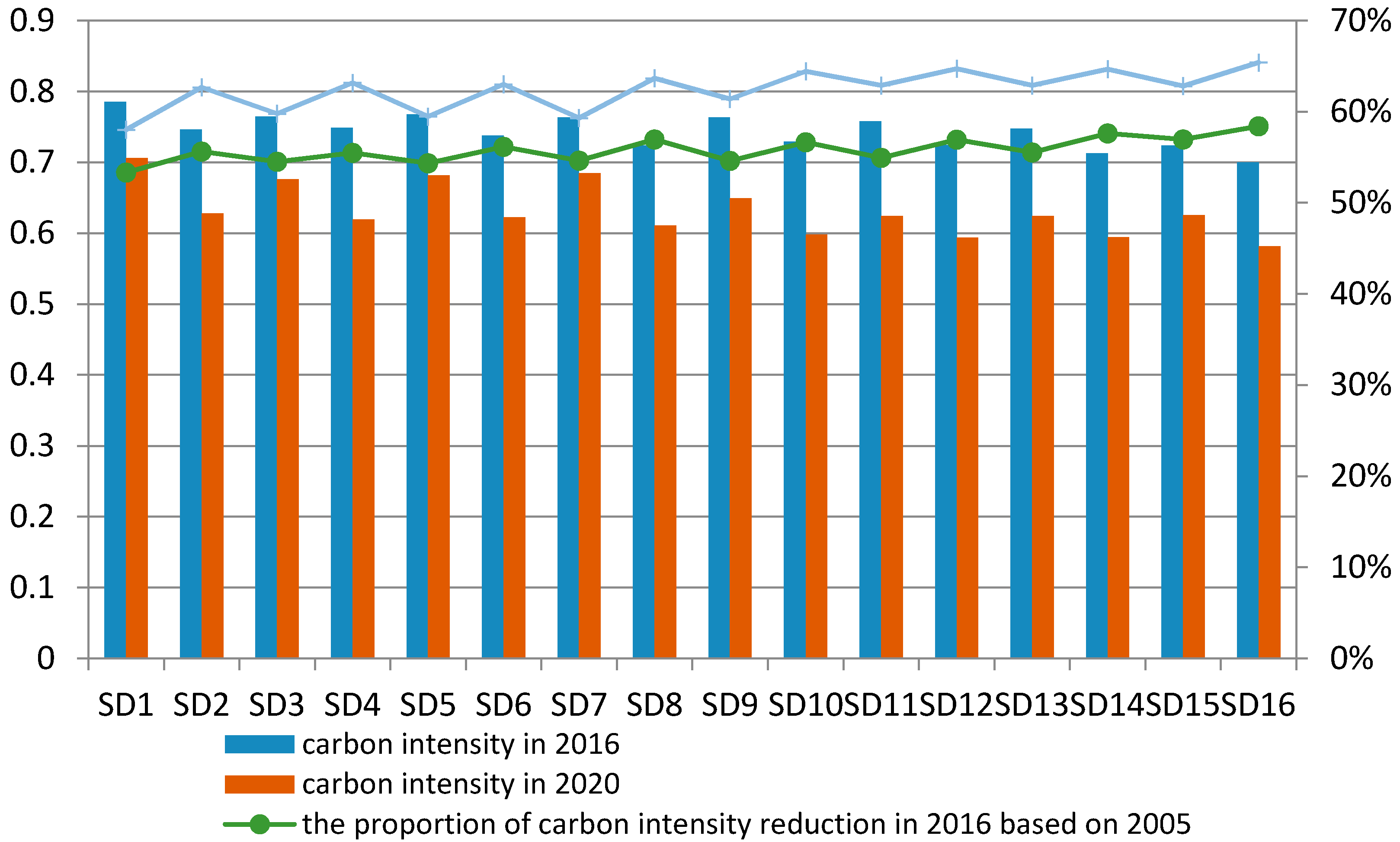
The strengthened development scenarios were comprised by 16 kinds of series, and the economic development of these series was set at the high rate. The predicted values of carbon intensity and the proportion of carbon intensity reduction of Beijing in 2016 and 2020 are shown in Figure 6.

The prediction results showed that the potential of carbon intensity reduction was more than 53% in 2016 and more than 55% in 2020 in the strengthened development scenarios. The potential of carbon intensity reduction can exceed the 40%–45% reduction target of carbon intensity in 2020 in all series. As far as the prediction values of 2016 and 2020 were concerned, carbon intensity would reach the peak in scenarios SD1, and the potential of carbon intensity reduction will achieve the minimum in scenarios SD1, in which the resident population growth rate was at the medium level and the change rate of energy structure, industrial structure and technical progress were at the low level. In addition, carbon intensity would reach the minimum value in scenarios SD16, and the potential of carbon intensity reduction would be at the peak in scenarios SD16, in which the resident population growth rate was at the low level and the change rate of energy structure, industrial structure and technical progress were at the high level, medium level and medium level respectively. The prediction results demonstrated that the lower population growth rate, the higher energy structure adjustment rate, the higher industrial structure adjustment rate and the higher technical progress rate contributed to lower carbon intensity. Nevertheless, the contribution of these influencing factors to carbon intensity was diverse. Through the comparison of SD2 and SD3, SD6 and SD7, SD11 and SD10, and SD15 and SD14, the contribution of technical progress on carbon intensity reduction was 2.2 times higher than that of industrial structure adjustment. Through the comparison of BD3 and SD5, and SD11 and SD13, the contribution of energy structure adjustment on the carbon intensity reduction was 15% higher than that of the industrial structure adjustment. Although the rate of energy structure adjustment was greater than that of technical progress, the comparison of SD1 and SD6, and SD9 and BD14 revealed that the contribution of technical progress on carbon intensity reduction was 1.6 times higher than that of energy structure adjustment. The growth of resident population went against the reduction of carbon intensity: the comparison of SD1 and SD9 indicated that if the resident population growth rate increased by 0.1%, the carbon intensity in 2020 would increase by 0.9%.

4.4. Comparison of Scenarios

Through comparison of the three development scenarios, we found that if the economic growth rate increased by 0.1%, the carbon emissions in 2020 would increase by 0.24%. However, there was no consistent relationship between carbon intensity and economic growth, and higher economic growth did not necessarily lead to higher carbon intensity. All three main scenarios demonstrated that the higher resident population growth meant the higher carbon intensity and the smaller potential of carbon intensity reduction. The contribution of technical progress to carbon intensity reduction was higher than the contribution of industrial structure adjustment in all of the scenarios. This might be attributed to the fact that the average annual change rate of technical progress and industrial structure adjustment were 3.65% and 0.65%, respectively. The contribution of energy structure adjustment to carbon intensity reduction was higher than that of industrial structure adjustment in three main scenarios. This might be attributed to the fact that the average annual adjustment rates of industrial structure and energy structure were 0.65% and 8%, respectively. The adjustment rate of industrial structure was less than energy structure. Although the energy structure adjustment rate was greater than the technical progress rate in three main scenarios, the contribution of energy structure adjustment to carbon intensity reduction was less than that of technical progress, which could be explained as follow: technical progress represents a decline in overall energy intensity; but the proportion of coal in primary energy consumption was only 18.16% in 2014; compared with the technical progress, the larger adjustment rate of energy structure cannot bring about the greater contribution to carbon intensity reduction. In conclusion, the energy structure adjustment and the technical progress made the greatest contribution to carbon intensity reduction, and they were the key factors of carbon intensity reduction for Beijing.

5. Conclusions and Policy Implications

5.1. Conclusions

In this study, IPSO-BP model was employed to calculate the carbon intensity of Beijing in 2016 and 2020. Based on different economic growth rates, resident population growth rates, energy structure adjustment rates, industrial structure adjustment rates and technical progress rates, this study set 48 development scenarios to explore the key influencing factors to the potential of carbon intensity reduction in 2016 and 2020.

From the analysis above, it can be concluded that Beijing can exceed the national target that carbon intensity will be reduced by 40%–45% by 2020 based on the 2005 level. The minimum carbon intensity reduction potential is 57.46%, which appears in the scenario OD1. The maximum carbon intensity reduction potential is 65.43%, which appears in the scenario SD16. In the three main scenarios, the lower resident population growth rate, the higher energy structure adjustment rate, the higher industrial structure adjustment rate and the higher technical progress rate will bring about the greater carbon intensity reduction potential, and energy structure adjustment and technical progress are the two major driving factors to carbon intensity decline.

5.2. Policy Implications

Based on the above conclusions, the following policy recommendations can be given to Beijing.

First of all, energy intensity should be kept falling, and comprehensive utilization efficiency of energy should be kept improving. Beijing should continue to promote energy conservation and emission reduction and further improve energy efficiency standards for different industries. Considering that the proportion of the tertiary industry in Beijing in 2014 has reached 77.9%, more attention should be given to energy efficiency in the tertiary industry, and the higher standards of energy efficiency should be formulated for key fields such as buildings, appliances and vehicles. In addition, Beijing should make full use of its rich resources of Higher Learning Institutions and further improve the level of cooperation between universities and enterprises to speed up the conversion efficiency of technology. Given that the developed countries have accumulated rich experience in energy-saving and emission-reduction, it is wise to learn experience and technologies from forerunners [38].

Secondly, energy structure should be kept optimizing. Effective measures are needed to further reduce the proportion of coal in primary energy and increase the consumption ratio of clean energy at the same time. The widely application of gas in households, industry and transport should be accelerated, as well as replacing coal with natural gas for heating in winter. Moreover, the proportion of coal-fired power generation should be lowered, and the vigorous development of non-coal power including gas, nuclear, wind, solar and waste incineration should be encouraged. The government should continue to provide tax incentives and financial subsidies to promote the development of renewable energy represented by wind energy and solar energy. The government should cooperate with the China State Grid Corp to accelerate the development of smart grid and distributed generation system to solve the difficult problem faced by renewable energy, such as hard to access the grid and high electric price level.

Thirdly, Beijing should continue to raise residents’ awareness of low-carbon and maintain a moderate speed of economic development to prevent the further growth of carbon emissions. Considering that the Chinese government pledged to reach the carbon emissions peak no later than 2030 at the climate conference in Paris, it is better for Beijing to convert the focus of carbon emissions reduction from carbon intensity to carbon emissions and promote carbon emissions reduction by means of market mechanism and administrative means.