Article

Energy Optimization in Smart Homes Using Customer Preference and Dynamic Pricing

1
COMSATS Institute of Information Technology, Islamabad 44000, Pakistan
2
School of Mechanical & Manufacturing Engineering, National University of Science and Technology, Islamabad 44000, Pakistan
3
Internetworking Program, Faculty of Engineering, Dalhousie University, Halifax, NS B3J 4R2, Canada
4
Cameron Library, University of Alberta, Edmonton, AB T6G 2J8, Canada
5
Department of Biomedical Technology, College of Applied Medical Sciences, King Saud University, Riyadh 11633, Saudi Arabia
*
Author to whom correspondence should be addressed.
Energies 2016, 9(8), 593; https://doi.org/10.3390/en9080593
Submission received: 19 November 2015 / Revised: 12 July 2016 / Accepted: 18 July 2016 / Published: 27 July 2016
(This article belongs to the Special Issue Energy Efficient City)

Abstract

:
In this paper, we present an energy optimization technique to schedule three types of household appliances (user dependent, interactive schedulable and unschedulable) in response to the dynamic behaviours of customers, electricity prices and weather conditions. Our optimization technique schedules household appliances in real time to optimally control their energy consumption, such that the electricity bills of end users are reduced while not compromising on user comfort. More specifically, we use the binary multiple knapsack problem formulation technique to design an objective function, which is solved via the constraint optimization technique. Simulation results show that average aggregated energy savings with and without considering the human presence control system are 11.77% and 5.91%, respectively.

Graphical Abstract

1. Introduction

In order to meet the ever-increasing energy demand, researchers investigate new research areas [1]: discovering new energy sources, distributed and renewable energy integration and energy saving programs by encouraging customers through demand side management (DSM) and demand response (DR) programs. Utilities participate in DSM programs to improve power system stability. On the other hand, end users participate in DR programs to minimize their electricity bills. Cost-sensitive customers can take monetary benefits by taking into consideration time varying prices and efficient scheduling techniques [2,3]. DR-based load shifting is helpful in reducing the electricity cost of end users, however, at the cost of user comfort. Similarly, the utility-based direct load control (DLC) technique improves power system stability [4], while disturbing user comfort. Thus, both cost reduction and comfort maximization cannot be achieved at the same time.
We identify that inconsideration of user activities in DSM and DR programs is the major cause of the earlier-mentioned trade-off. Furthermore, to utilize the available energy efficiently, unnecessary energy consumption must be reduced. Motivated by these considerations, this paper presents a new energy optimization technique to minimize the end user electricity bill while not compromising user comfort. In this paper, our contributions are listed as follows:
  • Initially, we categorize different homes and appliances by considering electricity prices, person occupancies and environmental conditions to manage energy consumption. Then, we propose mathematical optimization models of major household appliances to manage the energy consumption of all types of appliances. To maximize end user comfort, user-dependent appliances are introduced, which take into consideration human activities.
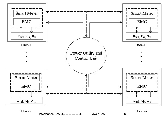
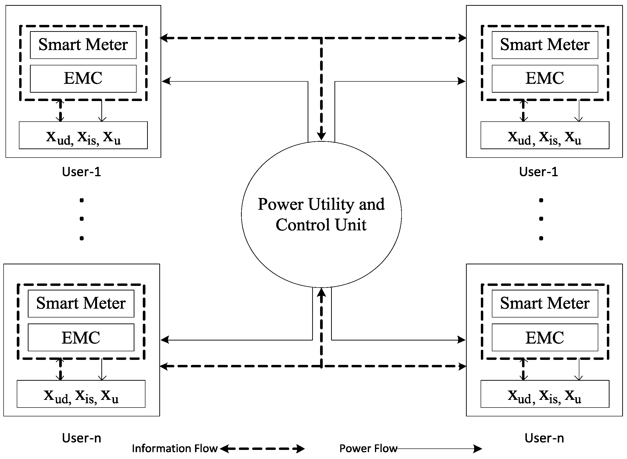
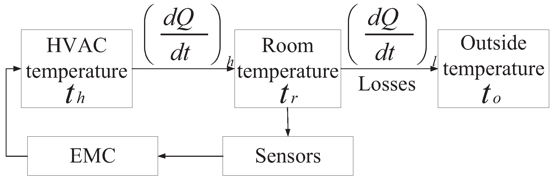
  • We propose a centralized energy optimization algorithm, which considers different constraints to minimize the overall energy consumption and electricity bill up-to ℏ homes (Section 4, Figure 1). However, prior to the selection and implementation of an optimization algorithm, different algorithms are tested and validated using the fmincon and lsqnonlin solvers (Table 3).
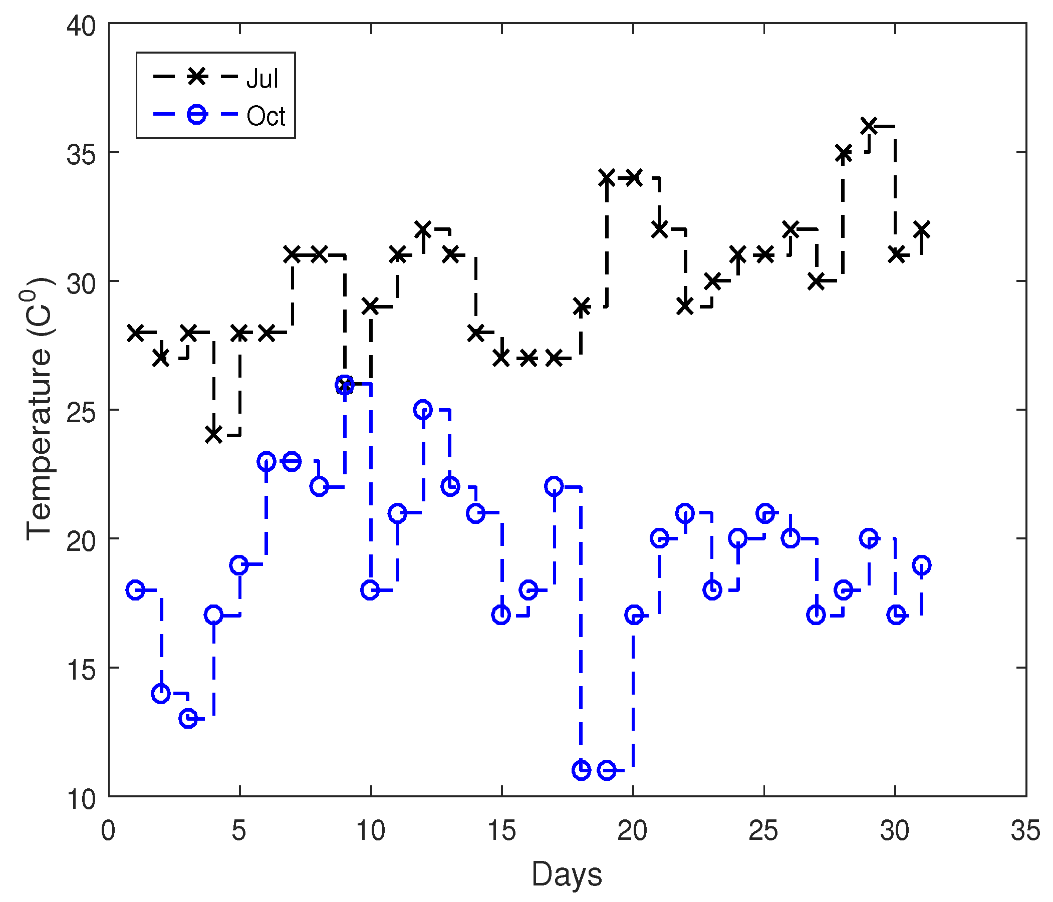
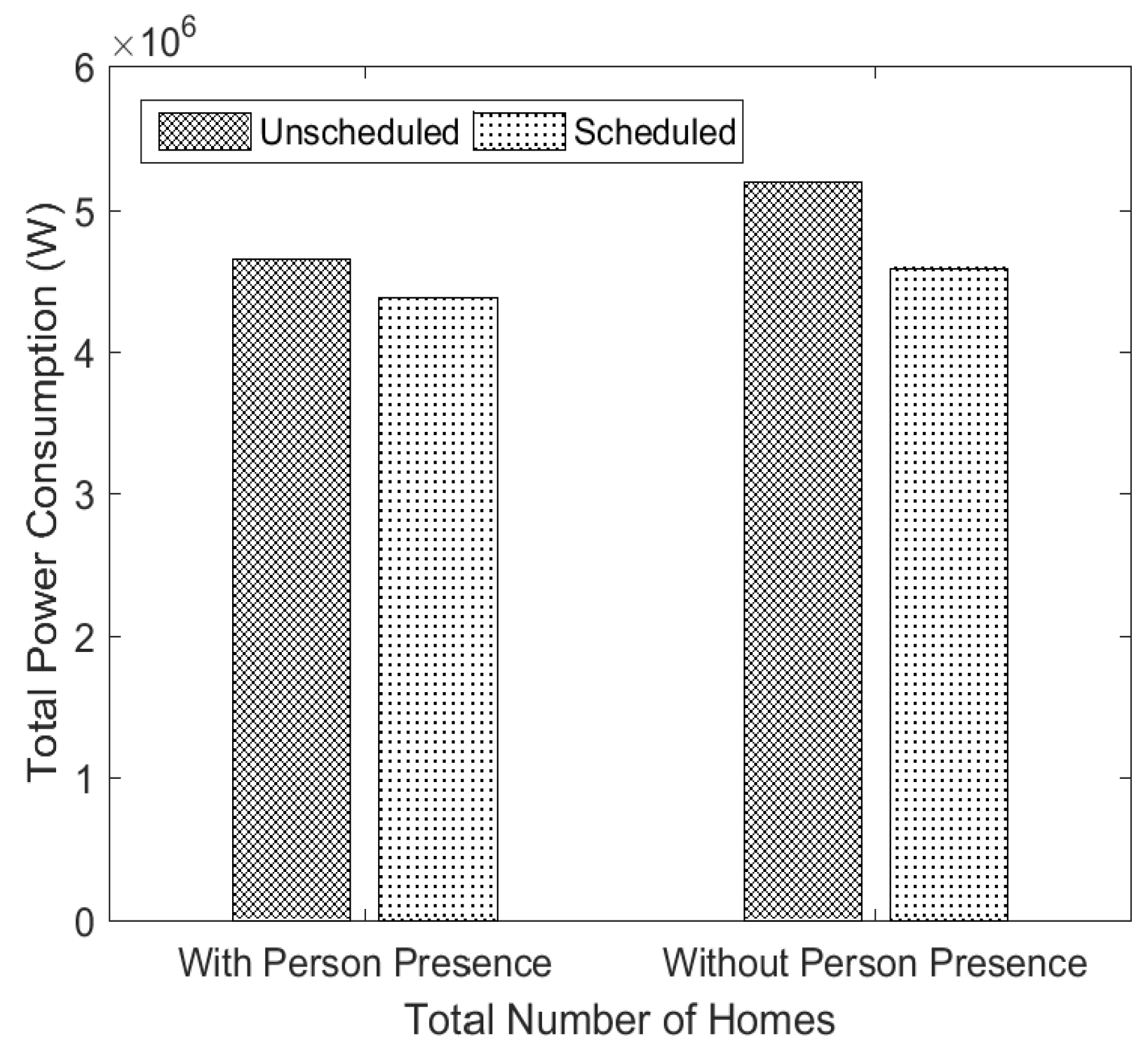
  • The influence of external temperature and variations in energy demand on DR programs is also analysed (details are given in Section 5.3). From this analysis, it is concluded that weather has a great impact on the energy consumption and DR programs based on which utilities and consumers manage their schedules.
  • Finally, extensive simulations have been performed to evaluate the effectiveness of the proposed algorithm in different scenarios.
The rest of the paper is organized as follows. Section 2 discusses the related work along with in-depth analysis of the state of the art work. The system model and appliance classification are discussed in Section 3. We then present the energy demand optimization in Section 4. Simulation results are discussed in Section 5. Initially, the simulation set-up and the solver users are discussed. Then, in-depth discussions of the obtained results and seasonal impacts on the energy consumption are discussed. Conclusions and future work are given at the end of the paper.

2. Related Work

In this section, we discuss the latest and relevant research work in two broader categories: (i) price based DR programs; and (ii) comfort-aware DR programs.
  • Price-based DR programs: Most of the published articles focus on DSM and direct load control (DLC) strategies to manage the energy demand during critical peak hours [2,3,4,5]. In these techniques, users may pause or turn-off unnecessary load to reduce their electricity cost. However, these techniques may disturb end user comfort. In [6], the authors have proposed a DR model under a dynamic pricing environment to reduce electricity cost and user discomfort. To maximize end user comfort, appliances are divided into different categories, such as deferrable, curtailable, thermal and critical. To reduce high peaks during low pricing hours, maximum energy consumption limits to restrict the customers to consume energy under the given limits are imposed. Users consuming more energy beyond these limits are charged high prices. In this work, again, the trade-off between user comfort and electricity cost reduction is found. However, the utility gains the benefit in terms of increased system stability. In another similar work, the authors introduce energy consumption limits in each time slot to reduce the electricity cost of end users [7,8]. Although this technique has shown a remarkable impact in terms of cost saving, the major drawback associated with this scheme are frequent disconnections and discouragement of consumers in participating in DR programs. In addition, users may feel discomfort while doing their daily life activities, because most of the DR programs are designed for grid stability and peak reduction [5,6,7,8,9].
    In [10,11], the authors consider only deferrable appliances, whereas [12] is limited to thermal loads only. In [13], a hybrid technique is proposed, which jointly controls the working of all, thermal, deferrable and non-interruptible, loads. In [14], mathematical models of various types of home appliances are proposed based on their energy demand and operating modes. After appliance classification, the energy management problem is formulated as a mixed integer nonlinear programming (MINLP) problem, which later on is solved using Benders’ decomposition approach. This scheme reduces the electricity cost with maximum appliance utility. However, user comfort has not been modelled in an effective way. In [15,16], the energy consumption of different types of appliances is managed, such that the major focus is on appliance scheduling, Peak to Average Ratio (PAR). and electricity cost reduction, as well as comfort management. However, a significant amount of energy is wasted due to unnecessary appliance operation. In [17,18], appliance scheduling schemes based on customer reward (CR) are proposed to avoid high peaks; customers are given incentives to shift load from on-peak hours to off-peak hours. However, comfort-aware customers cannot take full advantage of these types of schemes due to energy limits imposed by utilities. In conclusion, price based DR programs are efficient in reducing the electricity cost of end users along with PAR reduction, however at the cost of user comfort. The reason is the inconsideration of user behaviour in DSM programs.
  • Comfort-aware DR programs: In [19], a user comfort-aware load management algorithm is proposed to schedule the aggregate load of a household. The game theoretic approach is used to solve the optimization problem, aiming at minimizing end user cost while preserving end user comfort. Unlike the other schemes, this scheme gives users the choice to prioritize either comfort or electricity cost reduction. In [20], the authors present a user-aware game theoretic approach for demand management, which considers user preferences. Both hard and soft appliances are considered, including deferrable and non-deferrable categories, where users have options to either choose comfort or cost saving. For this purpose, the authors introduce a weight factor to prioritize comfort over cost. However, users cannot achieve both objectives at the same time. Moreover, appliance scheduling for minimum electricity cost may lead to high peaks during low pricing hours and may disturb user comfort [21]. In [22,23], the Markov chain is used to model a very limited set of user activities; using a personal computer, cooking activity and performing no activity. Based on these activities, total energy demand is calculated. Although these schemes prove to be efficient in terms of energy management, without the DR program, it is difficult to reduce end user cost. In [9], the authors schedule background loads, like refrigerator and humidifiers, by using the early deadline first technique. Non-background loads are not involved in the scheduling process, because these may affect user comfort. Each disconnected appliance is assigned a slack time, which is the maximum time for which any appliance remains disconnected from the power source. Afterwards, appliances with minimum slack time are turned-on. The authors also impose a power limit on aggregated power consumed by the background load. Although this scheme is efficient in terms of cost reduction, end user comfort is disturbed due to the high slack time of appliances and energy consumption limits.
Table 1 summarizes the work done by different authors along with their achievements and limitations. In conclusion, the techniques given in Table 1 are efficient in terms of cost reduction, but there management of energy with low electricity cost and high user comfort is not properly considered. These techniques do not consider both active human participation and environmental constraints, which are necessary for realistic scheduling and energy saving mechanisms. Keeping these limitations and trade-offs in view, we propose a demand side energy management algorithm, which takes into consideration dynamic prices, users preferences, weather conditions and active human participation.

3. System Model

We consider a home grid network, which consists of multiple residential units γ connected with a central Energy Management Controller (EMC) (Figure 1). In each residential unit γ, h number of homes is considered, such that each home is equipped with a smart meter to deliver the customer’s energy demand and preferences to the utility. The utility provides back the DR signal necessary for load scheduling and optimization. The smart meter can communicate directly with the centralized EMC and the utility. In each house, various types of appliances (e.g., human dependent, interactive schedulable and unschedulable) that have variable energy demand and operating time requirements are considered. The EMC aggregates operating schedules of household appliances and communicates with appliances using advanced communication technologies (e.g., Wi-Fi, ZigBee and Bluetooth). The EMC receives the information about human presence, weather conditions, price signals and appliance energy consumption requirements, based on which control decisions are made (Figure 2). In order to better schedule the load, we categorize home appliances based on operating time and energy consumption requirements (Table 2).

3.1. User Dependent

Major requirements of user dependent x u d appliances are to reduce end user cost, increase user discomfort and minimize uneven energy consumption [26,27]. An important aspect of this work is to control energy consumption of x u d based on human presence, electricity prices, weather conditions and operating time requirements. Example x u d appliances are: refrigerator, lights with controllable brightness, washing machine and Heating Ventilation and Air Conditioning (HVAC). In x u d , appliance utility function U ( E u d ( t ) ) denotes the overall performance when appliances consume E u d t amount of energy in time t. This is due to the fact that the electricity price in time interval t is a function of aggregated energy demand. In order to fulfil energy demand of x u d appliances, users have the following requirements.
E u d = t = 1 t n x = 1 n E ( t , x ) ψ ( t , x ) , x x u d .

3.1.1. HVAC

In HVAC modelling, we aim to design an algorithm that takes into consideration human presence/preference, temperature variations and maximum deviation in room temperature that a customer can bear. In h 1 , the HVAC is turned ON based on temperature difference only. On the other hand, the HVAC in h 2 is turned ON when occupants are present in the house and room temperature exceeds a threshold level (24 °C). In [23], the HVAC is turned on in low electricity pricing hours without considering human occupancy and temperature variations. For realistic scheduling (to achieve maximum user comfort), temperature difference and human occupancy parameters are considered in the proposed algorithm (Figure 3). The temperature of New York City based on which the proposed scheduling algorithm works is shown in Figure 4 [28]. Figure 4 shows that the maximum temperature in the month of July is 37 °C. On the other hand, the maximum temperature in October is 26 °C. Thus, the HVAC needs a relatively greater number of duty cycles to maintain room temperature in July due to the high temperature.
To model heat exchange between the HVAC and the outside, thermodynamic system modelling is used. Inside room temperature t r is defined as a state variable that allows us to model the temperature difference of a room in a thermodynamic system. Change in outside temperature t o leads to heat exchange ( d Q ( t ) d t ) l between the outside and inside, which is shown in Figure 3. This heat exchange disturbs internal room temperature t r . By using the energy management and control system in smart homes, t r can be controlled by considering user preferences and comfort requirements besides t o only, as used in [3,29]. For a given t r , users can change and control the HVAC temperature ( d Q ( t ) d t ) h set points through t h and then control t r .
By using the classical thermodynamics set of equations [26]:
d Q ( t ) d t h = M × C t h ( t ) t r ( t ) , t T .
d Q ( t ) d t l = t r ( t ) t 0 ( t ) r e q , t T .
Initially, r e q of the room is estimated based on the geometrical dimensions of the room, and later on, it is refined based on inside/outside temperature difference t r ( t ) t 0 ( t ) . Because r e q can change with varying material (walls and room) conductivity, the HVAC toggle condition is determined by the following condition:
d Q ( t ) d t h = 0 ; if t h ( t ) t r ( t ) ϱ O N / O F F ; if t h ( t ) t r ( t ) > ϱ .
where ϱ is a small quantity, whose value is 1 °C. In the first part of Equation (4), the temperature difference in the room is stable, and the scheduling algorithm will turn OFF the HVAC at time t and vice versa. The minimum and maximum temperature variations of t h are set as follows:
t h m i n t h t h m a x , t T .
Our objective here is to minimize heat losses that may change the room temperature. Due to more temperature variations inside the room, the HVAC needs a greater number of duty cycles to keep the temperature within the desired set points. Therefore, by reducing heat losses, the energy consumption of the HVAC can be significantly minimized. The heat losses minimization objective function is formulated as follows:
O b j = m i n t = 1 t n d Q ( t ) d t l ,
such that
h p = [ 0 , 1 ] ,
0 < t T ,
where h p denotes human presence in the room.
Remark 1. 
Referring to Algorithm 1, the HVAC turns on based on two conditions: (i) when there is any occupant in the room; and (ii) when there is a deviation in the temperature threshold. The only information required by the HVAC is the electricity price, which is obtained from New York Independent System Operator (NYISO) via the smart meter, room temperature and human occupancy through sensors.
Algorithm 1 Pseudo code of the HVAC working.
1: begin
2: Initialize parameters: t r , t t h , ϕ t
3: for all h = 1 : do
4:  for all t = 1 : T do
5:   if number of occupants > 0 and ( t d t t h o r t d t t h ) then
6:    solve objective Function (6)
7:    calculate E t
8:   else
9:    if number of occupants ≤ 0 and ( t d t t h ) then
10:      t o f f h
11:      t = t + 1 , go to Step 4; till T
12:    end if
13:   end if
14:  end for
15: end for
16: end

3.1.2. Refrigerator

We assume that the working of refrigerator can be scheduled throughout the day. In case of h 1 , energy consumption is calculated based on the length of operation time without taking into account the presence of a person [18,29]. In case of h 2 , the refrigerator performs on the bases of the total number of ON/OFF cycles and the total number of times the door is opened. Here, the total ON/OFF working cycles further depend on two factors: (i) heat losses when the refrigerator’s compressor is OFF; and (ii) the cooling effect when the refrigerator’s compressor is ON. On each attempt to open the door, the refrigerator consumes 20 W/h surplus energy to maintain inside temperature. Whereas the open and close operation of the refrigerator’s door d o is a random variable normally distributed over time t, so the objective is to maintain the refrigerator temperature within the comfort specified temperature limits along with minimum electricity cost. To achieve the aforementioned objective, the operational constraints of refrigerator are given as follows:
t r = h p t r ( t ) + τ [ Ψ r ( t ) + Φ r ( t ) + Υ r d o ( t ) ] , t T .
where:
  • t r = temperature of the refrigerator
  • t = time interval ( t 1 )
  • τ = duty cycle
  • Ψ r = heat losses during the OFF state
  • Φ r = cooling effect during the ON state
  • Υ r d o = heat loss due to d o .
Equation (7) shows the relationship of the refrigerator’s temperature at time interval t with the temperature at time interval t = ( t 1 ) , h p , heat Ψ r ( t ) losses and cooling Φ r ( t ) effects when the refrigerator is ON or OFF; where h p is calculated as follows:
h p = 1 ; if r a n d ( i ) 0 . 5 0 ; otherwise ,
Heat losses during the OFF state of the refrigerator are calculated as follows:
Ψ r = ϱ t r ϱ t ,
where ϱ t r is a small change in the refrigerator’s temperature in time interval t when the compressor is turned OFF. The cooling effect of the ON state of the refrigerator is calculated as:
Φ r = ϱ t r ϱ t + Ψ r ,
Our objective function here is to minimize the heat losses that may increase or decrease the refrigerator duty cycles.
O b j = m i n t = 1 t n Ψ r ,

3.1.3. Washing Machine

It is assumed that the working of the washing machine can be scheduled in 24 h. In γ 1 , the washing machine is turned ON once the low price time slot is found. In both homes, the scheduler adjusts the operating time of the washing machine between 01:00 → 09:00 and 17:00 → 09:00. In γ 2 , we assume that occupants stay home for the whole day. Therefore, the scheduler adjusts the operating time of the washing machine based on the presence of a person, as well as the total number of persons in the home. The following constraint is implemented while formulating the working of the washing machine.
h p ( 1 6 ) = μ s μ e ,
where μ s and μ e denote the start time and end time of the washing machine, respectively. h p ( 1 6 ) denotes the total number of occupants in the home, which is a random variable from ( 1 6 ) . The duty cycles of the washing machine depend on the h p ( 1 6 ) parameter in the second unit.

3.1.4. Lights with Controllable Brightness

The lighting of a house usually depends on the user occupancy/activity level and is modelled on the basis of the h p parameter. In both units, lights are assumed to be turned ON only when occupants are present in the home. The minimum and maximum energy consumption is 0 and 100 W, respectively.
l i g h t s = ON ; if h p = 1 OFF ; otherwise ,

3.2. Interactive Schedulable

These appliances, denoted by x i s , can be flexibly scheduled during the whole time period T. The energy consumption and user satisfaction of x i s appliances can be measured by the total E T amount of energy consumed in each time slot. The scheduler adjusts the working of x i s appliances in low price time slots. Appliances (dish washer and lights) without controllable brightness are kept in this category. For each appliance in x i s , users desire the following requirements to fulfil their needs.
t = 1 t n x i s = 1 n E ( t , x i s ) ζ ( t , x ) ,
where Equation (14) shows that the total energy consumption of all appliances cannot exceed the given limit ζ ( t , x ) .

3.2.1. Dish Washer

This appliance operates once in time period t T . In the first home, it operates during 07:00 → 12:00, because occupants are awake at this time. In order to reduce the electricity bill, the scheduler adjusts the working of the dishwasher in low price hours. In the second home, occupants are assumed to leave home from 09:00 → 05:00. The scheduler adjusts the working cycles of these appliances in low pricing time slots. In Unit 2, occupants are assumed to stay home during the whole day, and the scheduling algorithm calculates the working cycles (hours) of the dish washer based on the total number of persons in the home. The EMC automatically adjusts the working of the dishwasher to low pricing hours.

3.2.2. Lights without Controllable Brightness

For both households in Unit 1, the energy consumption of lights is 100 W. In the first home, the occupants are assumed to be awake from 07:00 → 24:00. In the second home, occupants leave the home from 09:00→ 05:00. In this case, EMC assigns time slots by considering electricity price and user preferences. In Unit 2, we assume that the occupants are present for the whole day. The EMC schedules the ON/OFF cycles based on the user presence at home.

3.3. Unschedulable

Appliances having fixed energy consumption, such as entertainment stations (TV, music player, etc.), are kept in the unschedulable x u category. In Unit 1, the operating time of these appliances is from 07:00 → 12:00 and from 05:00 → 07:00, respectively. In Unit 2, we assume that occupants stay home for the whole day, and the EMC schedules the appliances according to their presence. The minimum and maximum energy consumptions of these appliances are 0 and 1500 W, respectively.

4. Energy Demand Optimization

Our proposed algorithm takes into consideration the energy consumption of x u d appliances (HVAC and lights), such that these are controlled by considering user presence in the home. It is very difficult to predict accurate energy consumption demand in a house. One solution to solve this problem is to consider the real-time activities of occupants, based on which energy consumption can be calculated. The uncertain energy consumption patterns that depend on the daily activities of different users may create complexities in designing dynamic and interactive energy management algorithms. For example, the HVAC must be turned ON whenever the occupant is present in the room. On the other hand, scheduling techniques that is based on the DR signal may cause the wastage of energy. In the proposed work, x u d appliances are activated based on human presence, and the total cost during the ON time interval is calculated for these appliances. For x i s appliances, energy consumption is calculated in predefined schedules set by the users. However, these appliances can be scheduled during time slots t T to reduce the total electricity cost. The dish washer and lights with uncontrollable brightness are kept in this category. In the last category, x u has fixed energy consumption, and users can turn it ON at any time.

4.1. The Proposed Scheduling Algorithm

In the proposed model, we consider h homes having different types of χ appliances, such that χ = [ 1 , 2 , 3 , . . . N ] . Energy consumption schedules for all χ appliances are managed by the EMC, which takes price signals from the utility company via the smart meter (Figure 5). We use the Time of Use (TOU) and Real Time Pricing (RTP) signals in our case and divide the total scheduling time horizon T into time slots of the same length.
T = [ t 1 , t 2 , t 3 , . . . , t n ] ,
where t n is equal to 24. The EMC is responsible for determining the starting ( t s ) and ending ( t e ) time intervals, as well as the total energy consumption E t of χ appliances. Over a given sub-interval of time t 1 , the energy consumption is assumed to be constant. Energy consumption scheduling vector E x for appliance x χ is given as:
E x = [ e x t 1 , e x t 2 , e x t 3 , . . . , e x t n ] ,
where E x denotes the energy consumption of appliance x at t t h time slot in kWh. Considering the TOU price signal, as shown in Figure 5, and appliance classification, the energy consumption value is fixed in each time slot. Each appliance x has a scheduling time interval t s c h [ t s , t f t l o t ] in which it can be scheduled.
When appliance x is ON, its energy consumption E is bounded between minimum and maximum bounds, E x m i n and E x m a x , respectively.
E ( x , t ) m i n ψ ( x , t ) E ( x , t ) E ( x , t ) m a x ψ ( x , t ) ,
where ψ ( x , t ) denotes the ON/OFF status of appliance x at time slot t. The appliance ON/OFF mechanism manages the scheduling process more realistically as compared to simple time-based models discussed in [30,31]. For example, if a user wants to stop any appliance during high price hours 08:00 → 10:00, the ON/OFF mechanism is easy to model. If a user in need models the time horizon by introducing additional variables, this creates complexity.
ψ ( x , t ) = 1 ; if appliance x is ON at time slot t 0 ; otherwise
The energy consumed by χ number of appliances in time t is calculated as follows:
E t = h = 1 t = 1 t n x = 1 n E ( t , x ) . ψ ( t , x ) .
where E t is total energy consumed by x number of appliances in time t. It is also assumed that each appliance has maximum energy consumption limit E m a x t in time slot t. For example, the washing machine may consume 3 . 4 kWh of energy in each hour, such that E x t E m a x x t . Where E x t denotes the energy consumed by appliance x at time t. Additionally, there is also a total energy consumption limit ζ t on all types of appliances in each time slot t n , which is calculated by the following equation.
h = 1 t = 1 t n x = 1 n E ( t , x ) . ψ ( t , x ) ζ ( t , x ) .
Violation of above constraint leads to the possibilities that high peaks will be generated, which may damage the power grid. The scheduling algorithms must follow the capacity constraint (for smooth gird operation) and the generation cost of electricity to fulfil the energy demand during low price hours. After describing appliance energy consumption and capacity limits, we now formulate the energy consumption cost. We use TOU and RTP pricing models in which electricity price varies in each time interval t and is denoted by ϕ t . We also assume that all electricity unit prices ϕ t for the scheduling intervals are known to the EMC in advance. The total energy consumption cost C T for all types of appliances is given as:
C T = h = 1 t = 1 t n x = 1 n E ( t , x ) . ϕ ( t , x ) .

4.2. Load Scheduling

The main purpose of this model is to reduce the energy consumption by taking into consideration human presence, weather conditions and energy prices. In order to reduce the electricity bill and high peaks during low price hours, appliances are scheduled on the bases of energy prices and capacity limits. The final optimization problem for energy consumption minimization is given as follows:
O b j = m i n h = 1 t = 1 t n x = 1 n E ( t , x ) . ψ ( t , x ) .
such that:
0 t T ,
t s c h = [ t s , t f t l o t ] ,
E t ζ t ,
E ( x , t ) m i n ψ ( x , t ) E ( x , t ) E ( x , t ) m a x ψ ( x , t ) ,
ψ = [ 0 , 1 ] ,
where Constraint (22a) shows that t s and t f must be within the total time limit t T . Constraint (22b) defines the total scheduling time horizon. Constraint (22c) bounds the total energy consumed by all types of appliances not to exceed the available energy capacity. As per Constraint (22e), the appliance has two possible states, ON and OFF. In the case of the ON state, its energy consumption follows (22d).

4.3. PAR Reduction

The daily energy consumption of the x-th appliance in time slot t is given as follows:
E = t = 1 t n x = 1 n E ( t , x ) . ψ ( t , x ) .
Given the maximum energy load demand vector E t , x , we formulate PAR in terms of average load demand as follows:
PAR = max t t n x = 1 n E ( x ) 1 T x = 1 n E ( x ) .
The PAR reduction optimization problem can be formulated as follows:
O b j = m i n PAR .

5. Performance Evaluation

In this section, we present the simulation results and discussions of the proposed energy management algorithm. We first describe the simulation set-up and performance metrics and then discuss the proposed algorithm used to solve the optimization problem. Finally, simulation results considering different cases are discussed in terms of selected performance metrics.

5.1. Simulation Set-Up

The performance of the proposed energy optimization algorithm is evaluated under TOU and RTP pricing environments. We consider two residential units having two homes in each unit. In Unit 1, occupants stay home for the whole day in h 1 . In h 2 , occupants are assumed to leave for the office from 07:00 → 05:00. In Unit 2, the occupants stay home for the whole day. In h 1 , the working of appliances is scheduled without considering user presence. In h 2 , appliances are scheduled by taking into consideration the customers presence, preferences, total number of persons in the home and weather conditions.
In Scenario 1, we set γ = 2, h = 2 and χ = 7 . Furthermore, winter and summer seasons are also considered to evaluate the impact of variable energy demand on the DR program. In Scenario 2, ten different users are considered, and the proposed algorithm is used to evaluate the energy consumption variations based on its usage. In Scenario 3, the total number of houses and appliances is increased to h = 40, and χ = 280 , and the robustness of the proposed algorithm is tested. Each appliance has different energy consumption requirements, which mainly depend on the appliance type and power rating, as shown in Table 2. We consider a T = 24 h time horizon, which is further subdivided into different time slots, each one of the same length t l . Alternatively, higher energy demand is observed in the evening because most people return home from offices. On the other hand, lower energy demand is observed at night because most of the people sleep during this interval. We simulate the proposed model considering different scenarios where user preferences, weather conditions and electricity prices vary. Electricity prices are taken directly from [32]. We use MATLAB to implement the proposed model and evaluate the performance of the proposed algorithm. To perform optimization, we use the MATLAB solver f m i n c o n to solve the energy management problem. We simulate and analyse the performance of different algorithms used in this solver as shown in Table 3.

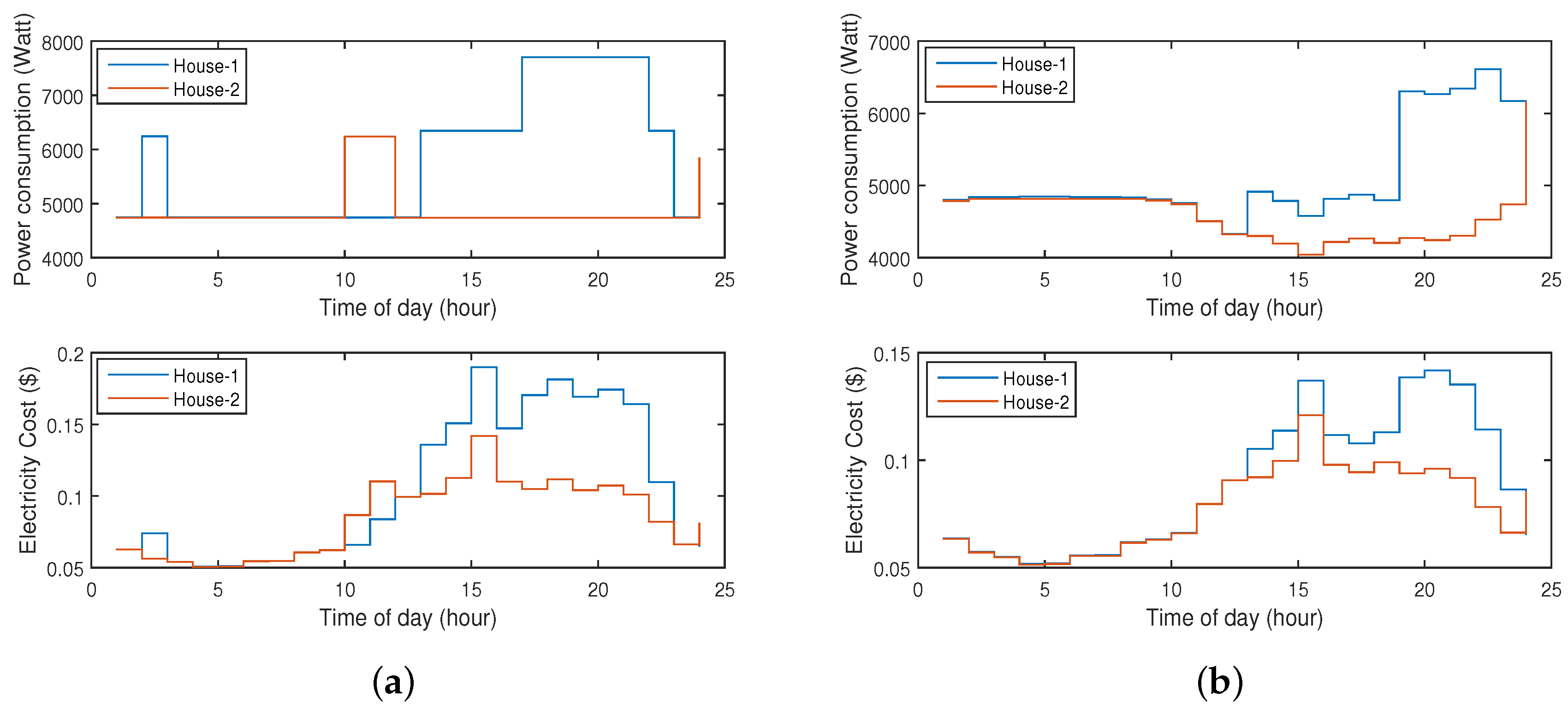
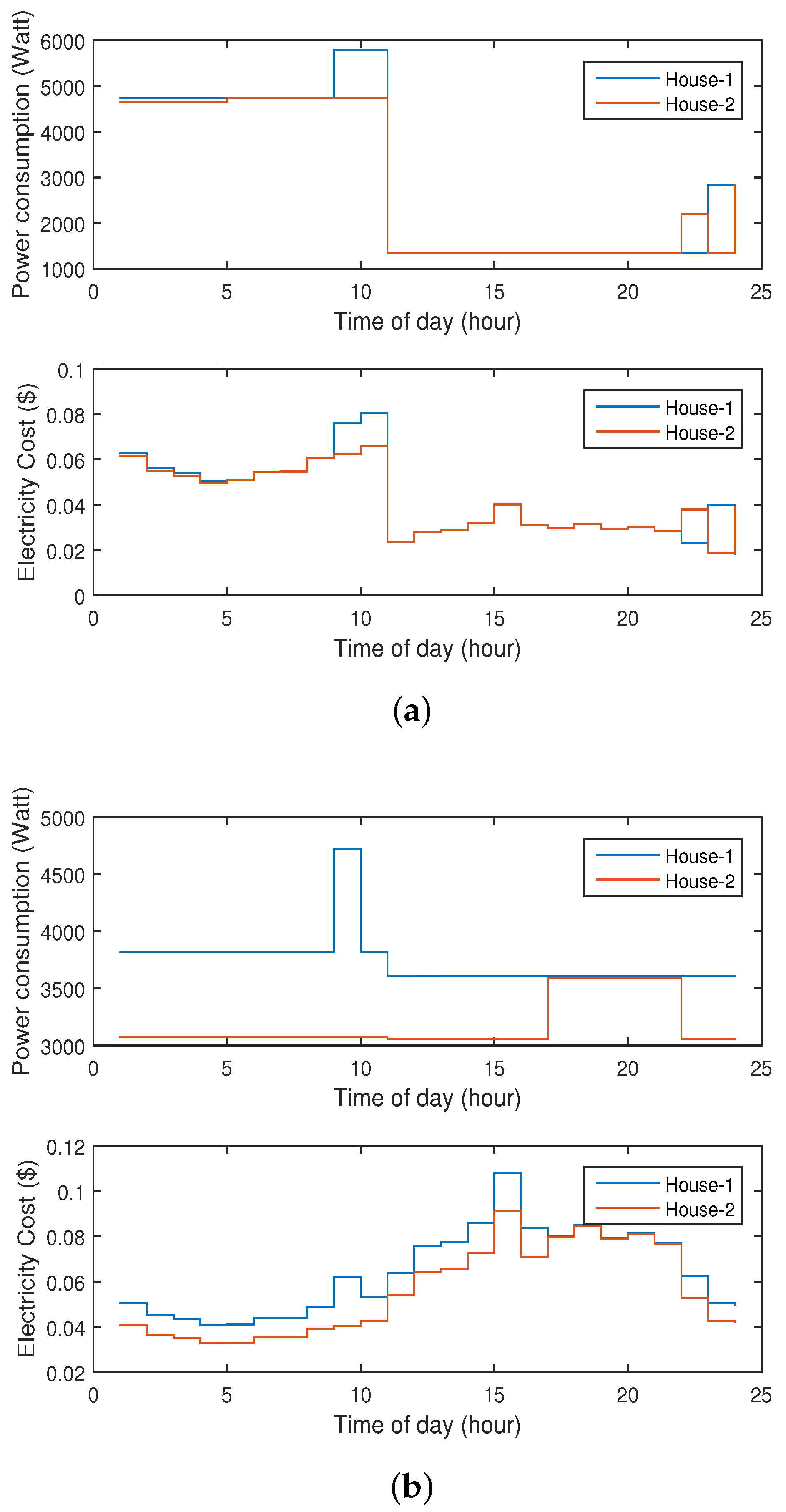
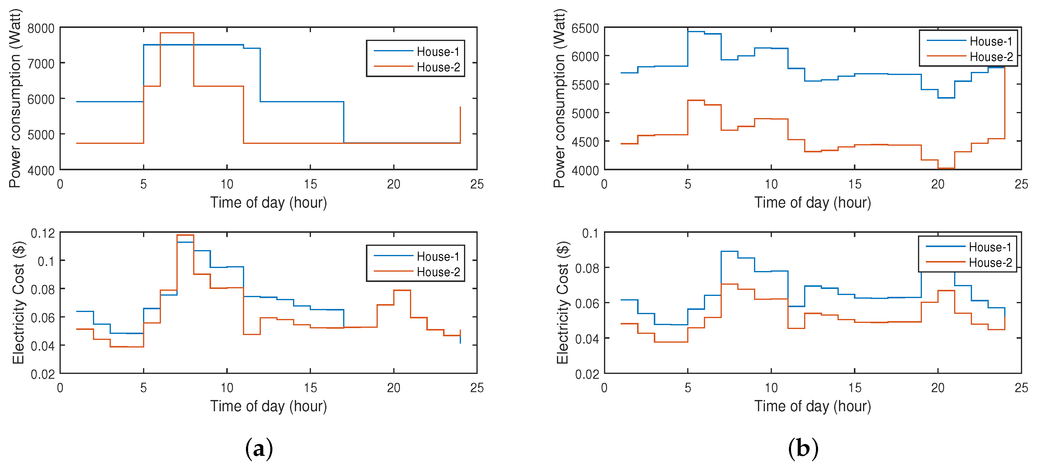
5.2. Results and Discussion

Figure 6a shows the comparison of the unscheduled energy consumption and electricity cost of both homes. Here, the energy consumption of both homes is almost the same, except time slots 07:00 → 08:00 and 12:00 → 17:00, in which h 1 consumes 4.03% more energy. Figure 6b compares scheduled energy consumption and electricity cost, where h 1 consumes more energy during time slot 08:00 → 11:00, which is comparatively 5.03% higher. In Figure 7b, h 1 consumes more energy during time slot 15:00 → 18:00, because occupants return home after office 09:00 → 05:00, and they are supposed to turn the maximum load ON, such as the HVAC, the TV, the oven, etc. (refer to Section 3). In general, h 2 consumes 23.14% less energy as compared to h 1 .
It is clear from Figure 8a that h 1 consumes 14.73% more energy than h 2 in the unscheduled case. Because in Unit 2, appliances are randomly turned ON and OFF in the scheduling time horizon, the EMC adjusts the working cycles of all appliances based on low electricity pricing time slots without considering human occupancy and user preferences. Figure 8b shows the comparison of the scheduled energy consumption and the electricity cost of both homes. During peak hours 09:00 → 11:00, h 1 consumes 7 kW/h in the unscheduled case, and h 2 consumes 5 kW/h in the scheduled case, which is 7.42% less. However, h 1 consumes 2.97% more energy as compared to h 2 . This is because some appliances are turned ON during high price hours due to person presence. Electricity prices from 19:00 → 24:00 are very low. Due to critical peak hours 19:00→ 24:00, Figure 5, the EMC tries to schedule most of its load during low price hours to save on the electricity bill. The low electricity bill in h 2 is due to the fact that the scheduler generates the appliances’ ON/OFF patterns on the basis of user presence, the t s and t f parameters.
Figure 9 shows the comparison of the unscheduled and scheduled cost and power consumption in the RTP environment. Unscheduled power consumption in both homes is almost 8 kW/h during high price hours 07:00 → 11:00. The scheduled power consumption in h 1 is from 6 to 7 kW/h, which is 23% less than h 2 . In h 2 , the scheduled power consumption during 16:00 → 18:00 is high, as compared to time slots 01:00 → 16:00 and 18:00 → 24:00. The total power consumption of h 2 is 16.11% less than h 1 . The unscheduled energy consumption of h 1 is 5.74% more than h 2 , and the scheduled energy consumption of h 1 is 23.11% more than h 2 , respectively.
These savings reflect the effectiveness of human occupancy and user preference parameters, as discussed in Section 3. In the RTP environment, prices vary in each time slot due to real-time data exchanged between the utility and consumers. These variations may create complexities in constructing a cost-effective energy management algorithm. Thus, our proposed algorithm is effective in terms of energy and cost reduction. Table 4 and Table 5 show the percentage of total electricity cost and energy saving in both the TOU and RTP environments. The overall cost savings of h 1 and h 2 are 40.57% and 60.92%, respectively. It is clear from the tables that the total electricity cost saving of h 2 is 33.41% more than h 1 due to the incorporation of human presence control and weather condition parameters.

5.3. Impact of Seasons on the Energy Optimization

In order to analyse the impact of energy consumption trends on the DR program, we consider summer and winter seasons. The average outside temperatures in the months of July and October 2015 are shown in Figure 4 [5]. The outside temperature has significant impact on DR programs due to energy demand variations, especially due to HVAC systems, which consume almost 60% of the overall energy. The energy consumption schedules of household appliances in summer are shown in Figure 10. It is clear from Figure 10a that almost a constant amount of energy is consumed by both households during 01:00 → 12:00. From 13:00 → 23:00, h 1 consumes more energy as compared to h 2 due to energy demand variations. h 2 consumes 14.69% less energy in comparison to h 1 . This reduction is due to x u d appliances, which are only turned ON when occupants stay home. Figure 10b clearly shows that the EMC shifts some load from 13:00 → 19:00 to other time slots to reduce cost and peak load due to capacity limits (Equation (13)). The energy consumption of h 2 is relatively less due to the activity recognition system. In h 1 , the working of the HVAC is controlled on the basis of inside/outside room temperature differences given in [3,29,30,31,32,33]. In h 2 , human presence along with outside/inside temperature difference is also incorporated in controlling the temperature set points of the HVAC. Figure 11 shows the energy consumption analysis of different homes based on the DR signal for October 2015. It can be analysed from Figure 12 and Figure 13 that occupants consume 5.51% more energy in October as compared to July. However, the total electricity cost in October is relatively less (6.66%).

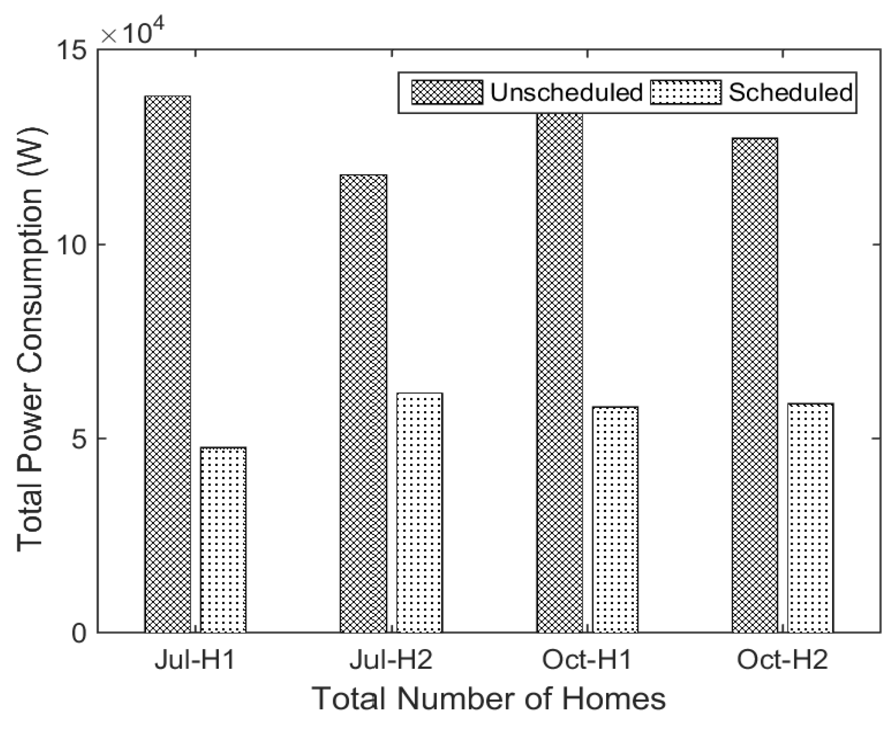
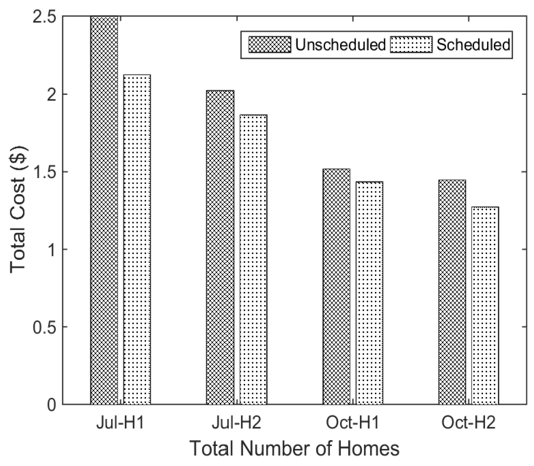
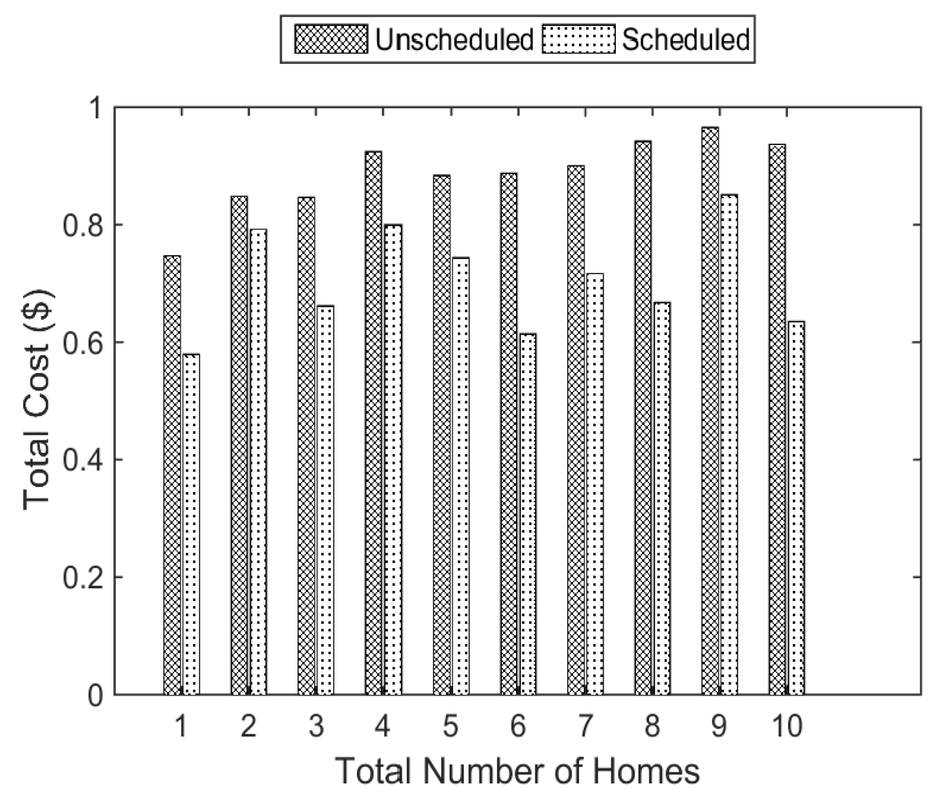
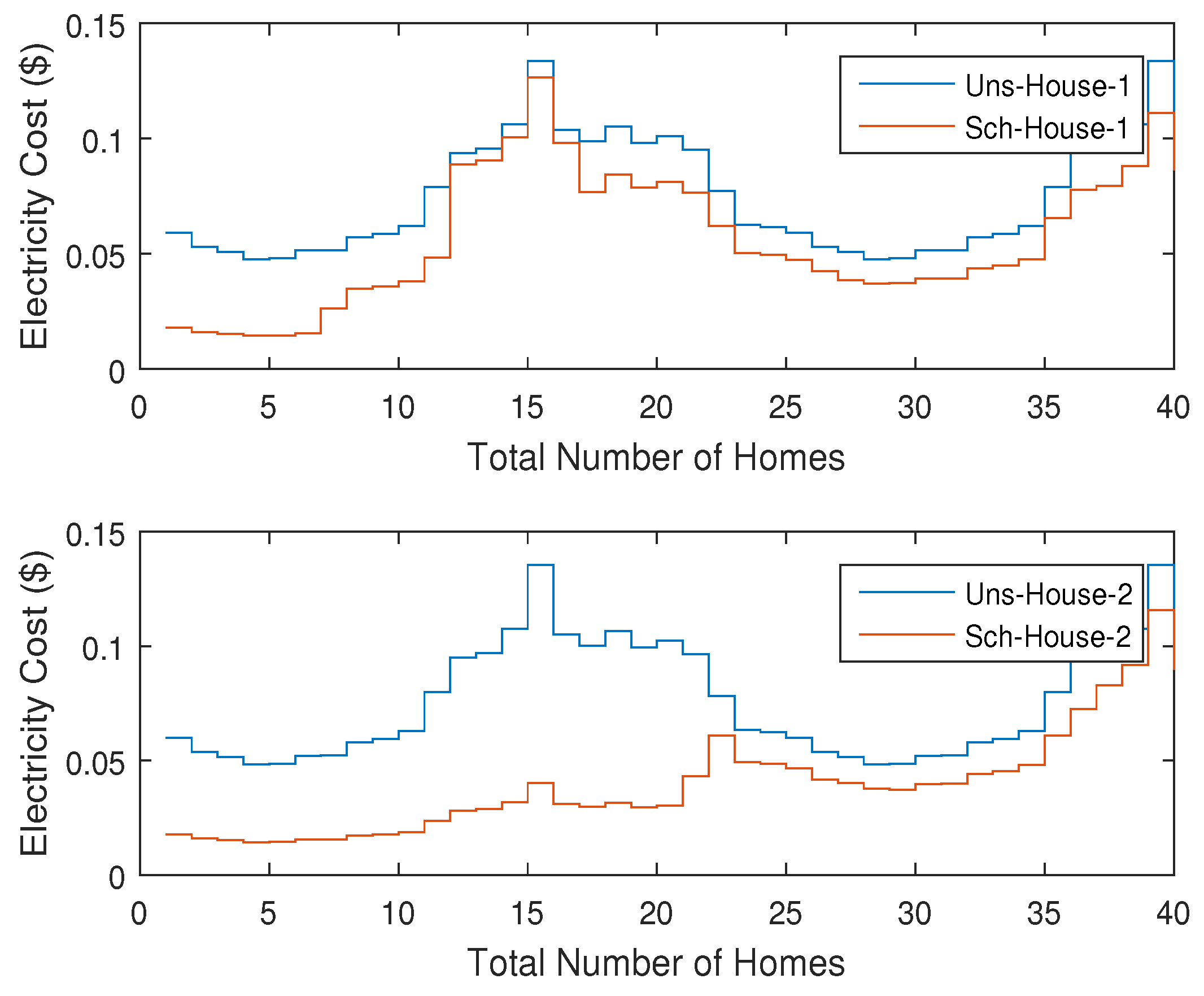
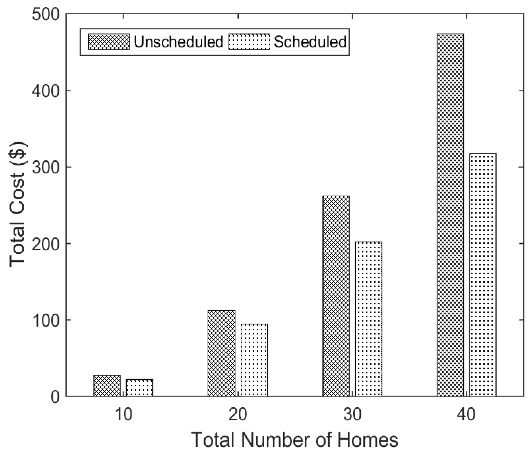
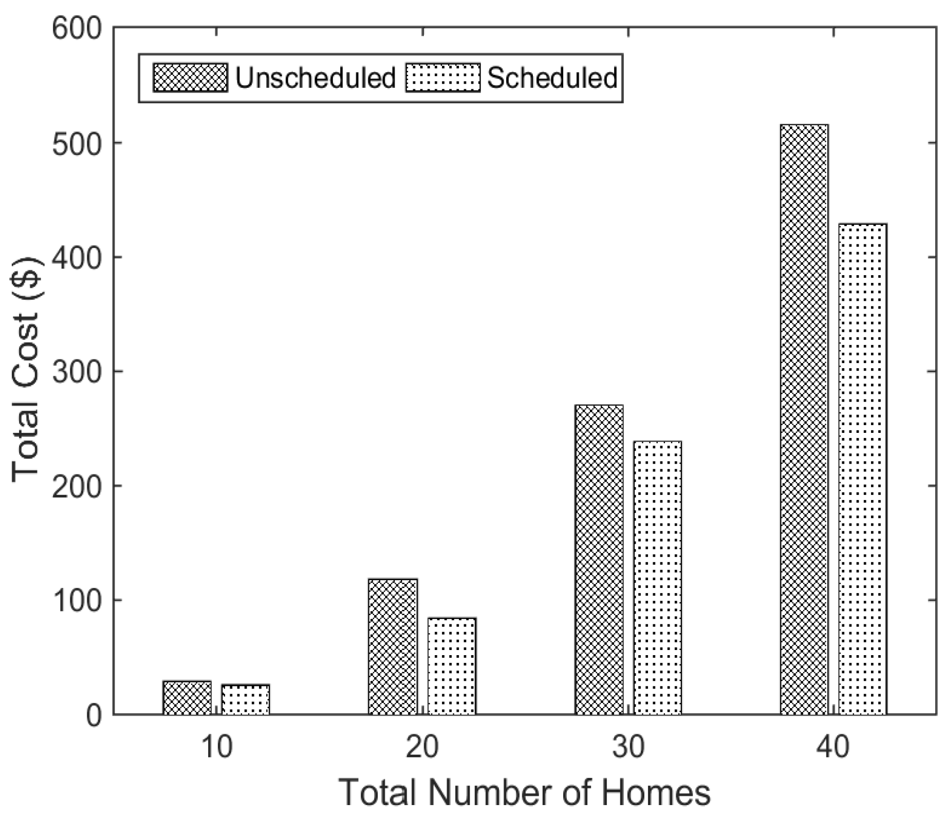
5.4. Impact of Number of Homes
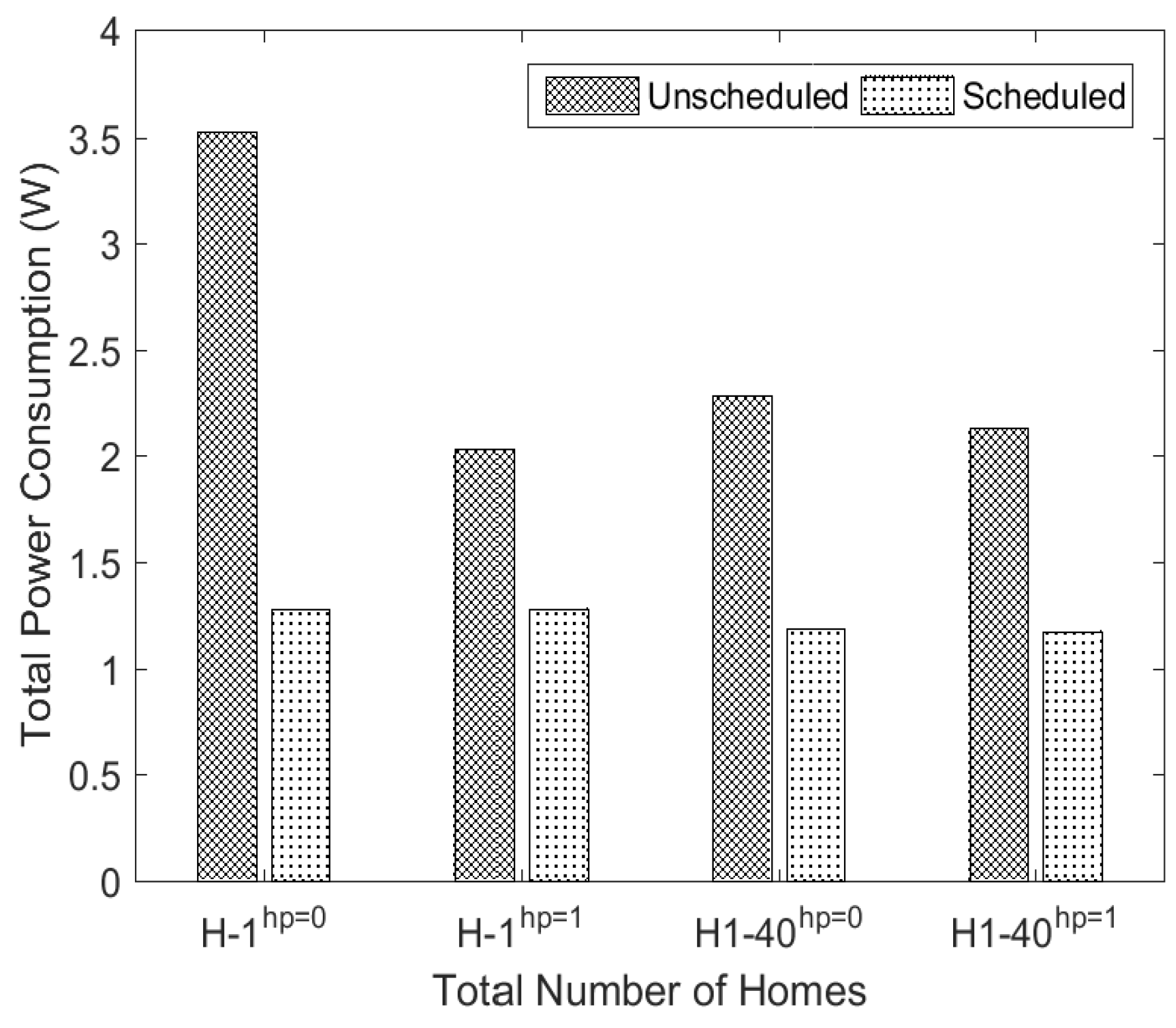
In this sub-section, we extend our analysis from only one home to 40 homes. Firstly, the proposed algorithm is implemented for 10 users, and its performance is analysed. Figure 14 shows varied electricity cost as the number of homes is increased from one to 10. This is due to the fact that all users have different energy consumption requirements and living patterns, so the electricity prices are different. Secondly, the performance of the proposed algorithm is evaluated for 40 homes, where Figure 15 and Figure 16 show the total electricity cost and energy consumption. The aggregated bill reduction of 40 homes with and without person presence control is 92.85% and 68%, respectively, which is shown in Figure 17 and Figure 18. On the other hand, 11.77% and 5.91% of the total energy consumption is reduced with and without person presence control, respectively. It is clear that our proposed algorithm is able to manage the energy consumption for a large number of homes and variable loads. Some users may get more benefits on the electricity bill if they consume less energy, because the energy consumption of each appliance is considered separately in the proposed algorithm.

5.5. Impact of PAR

In this section, we analyse the impact of our proposed energy management algorithm on total PAR reduction, which is an important parameter for electricity providers. The EMC performs appliance scheduling based on Objective (24) to minimize PAR. Figure 19 shows the comparison of total PAR reduction in scheduled and unscheduled cases. It is clear that our proposed algorithm significantly reduces the average PAR of a single home and 40 homes. In the case of a single home with h p = 1 , the average PAR reduction is 25%, while the average PAR reduction is 47.62% in the case of 40 homes.

6. Conclusions and Future Work

In this paper, we have identified that the inconsideration of user activities in the existing scheduling techniques creates a trade-off between energy consumption minimization and user comfort maximization. Direct involvement of user activities in our proposed load optimization technique relaxed the trader-off between user comfort and the electricity bill. Considering this trade-off, optimization models of different household appliances have been proposed and implemented by using the proposed algorithm (Section 4.1). The simulation results are analysed in terms of the reduction in energy consumption, the reduction in cost and occupancy. Table 5 shows that a single home saves electricity cost up to 28.85%, whereas 16.80% of the cost is saved in the case of 40 homes, while 25% and 47.62% PAR reductions are achieved in a single and 40 homes, respectively. The unscheduled energy consumption of h 1 is 5.74% more than h 2 , and the scheduled energy consumption of h 1 is 23.11% more than h 2 . Moreover, the analysis of the impact of seasons on the DR programs is beneficial for utilities in managing electricity generation according to variations in demand.
In the future, we will extend this work for a complete residential unit, where: (i) advanced forecasting techniques will be used to estimate total load demand and the availability/capacity of distributed energy resources (solar and wind); and (ii) energy management algorithms will be developed by integrating distributed energy resources into the local microgrid through multi-agent coordination and control techniques [34,35].

Acknowledgments

The authors would like to extend their sincere appreciation to the Deanship of Scientific Research at King Saud University for funding this Research group No. RG-037-1435.

Author Contributions

Muhammad Babar Rasheed, Nadeem Javaid, and Ashfaq Ahmad did and wrote simulations after classifying the appliances and proposing the time slots. They performed mathematical formulations as well. Mohsin Jamil, Zahoor Ali Khan, Umar Qasim and Nabil Alrajeh tracked overall work flow, set & refined the manuscript, and then revised the manuscript according to the reviewers’ comments.

Conflicts of Interest

The authors declare no conflict of interest.

Nomenclatures

SymbolDescriptionSymbolDescription
x u d user-dependent appliances ϕ t electricity unit price
x i s interactive schedulable appliancesψappliance ON/OFF status
x u unschedulable appliancesTtotal time horizon
γresidential unitsζenergy consumption threshold
E c o n m i n minimum energy consumptionχappliance set
E c o n m a x maximum energy consumption h p = [ 0 , 1 ] human presence
t h m i n minimum temperature t h m a x maximum temperature
t s c h scheduling horizon t s appliance starting time
E t total energy consumption λ a Boolean variable for ON/OFF status
ϱsmall change in temperature r e q equivalence resistance of room
MHVAC air flow rateCspecific heat capacity
d Q d t ( t ) heat exchange t o outside temperature
t r room temperature U ( E t ) appliance utility function s
C T total electricity costCelectricity cost
t f appliance finishing time h homes
t h HVAC temperature t d temperature difference

References

  1. Bose, B.K. Global Warming: Energy, Environmental Pollution, and the Impact of Power Electronics. IEEE Ind. Electron. Mag. 2010, 4, 6–17. [Google Scholar] [CrossRef]
  2. Ye, F.; Qian, Y.; Hu, R.Q. A Real-Time Information Based Demand-Side Management System in Smart Grid. IEEE Trans. Parallel Distrib. Syst. 2016, 27, 329–339. [Google Scholar] [CrossRef]
  3. Rasheed, M.B.; Javaid, N.; Ahmad, A.; Khan, Z.A.; Qasim, U.; Alrajeh, N. An Efficient Power Scheduling Scheme for Residential Load Management in Smart Homes. Appl. Sci. 2015, 5, 1134–1163. [Google Scholar] [CrossRef]
  4. Salehfar, H.; Patton, A. Modeling and evaluation of the system reliability effects of direct load control. IEEE Trans. Power Syst. 1989, 4, 1024–1030. [Google Scholar] [CrossRef]
  5. Sianaki, O.A.; Hussain, O.; Tabesh, A.R. A Knapsack problem approach for achieving efficient energy consumption in smart grid for endusers’ life style. In Proceedings of the IEEE Conference on Innovative Technologies for an Efficient and Reliable Electricity Supply (CITRES), Waltham, MA, USA, 27–29 September 2010.
  6. Althaher, S.; Mancarella, P.; Mutale, J. Automated demand response from home energy management system under dynamic pricing and power and comfort constraints. IEEE Trans. Smart Grid 2015, 6, 1874–1883. [Google Scholar] [CrossRef]
  7. Costanzo, G.T.; Zhu, G.; Anjos, M.F.; Savard, G. A system architecture for autonomous demand side load management in smart buildings. IEEE Trans. Smart Grid 2012, 3, 2157–2165. [Google Scholar] [CrossRef]
  8. Pipattanasomporn, M.; Kuzlu, M.; Rahman, S. An algorithm for intelligent home energy management and demand response analysis. IEEE Trans. Smart Grid 2012, 3, 2166–2173. [Google Scholar] [CrossRef]
  9. Barker, S.; Mishra, A.; Irwin, D.; Shenoy, P.; Albrecht, J. Smartcap: Flattening peak electricity demand in smart homes. In Proceedings of the IEEE International Conference on Pervasive Computing and Communications (PerCom), Lugano, Switzerland, 19–23 March 2012; pp. 67–75.
  10. Zhao, Z.; Lee, W.C.; Shin, Y.; Song, K.B. An optimal power scheduling method for demand response in home energy management system. IEEE Trans. Smart Grid 2013, 4, 1391–1400. [Google Scholar] [CrossRef]
  11. Chen, X.; Wei, T.; Hu, S. Uncertainty-Aware household appliance scheduling considering dynamic electricity pricing in smart home. IEEE Trans. Smart Grid 2013, 4, 932–941. [Google Scholar] [CrossRef]
  12. Lin, Y.H.; Tsai, M.S. An Advanced Home Energy Management System Facilitated by Nonintrusive Load Monitoring with Automated Multiobjective Power Scheduling. IEEE Trans. Smart Grid 2015, 6, 1839–1851. [Google Scholar] [CrossRef]
  13. Chen, C.; Wang, J.; Heo, Y.; Kishore, S. MPC-Based appliance scheduling for residential building energy management controller. IEEE Trans. Smart Grid 2013, 4, 1401–1410. [Google Scholar] [CrossRef]
  14. Roh, H.T.; Lee, J.W. Residential Demand Response Scheduling with Multiclass Appliances in the Smart Grid. IEEE Trans. Smart Grid 2016, 7, 94–104. [Google Scholar] [CrossRef]
  15. Liu, Y.; Yuen, C.; Huang, S.; Hassan, N.U.; Wang, X.; Xie, S. Peak-to-Average Ratio Constrained Demand-Side Management with Consumer’s Preference in Residential Smart Grid. IEEE J. Sel. Top. Signal Process. 2014, 8, 1084–1097. [Google Scholar] [CrossRef]
  16. Mahmood, D.; Javaid, N.; Alrajeh, N.; Khan, Z.A.; Qasim, U.; Ahmed, I.; Ilahi, M. Realistic Scheduling Mechanism for Smart Homes. Energies 2016, 9, 202. [Google Scholar] [CrossRef]
  17. Vivekananthan, C.; Mishra, Y.; Ledwich, G.; Li, F. Demand response for residential appliances via customer reward scheme. IEEE Trans. Smart Grid 2014, 5, 809–820. [Google Scholar] [CrossRef]
  18. Setlhaolo, D.; Xia, X.; Zhang, J. Optimal scheduling of household appliances for demand response. Electr. Power Syst. Res. 2014, 116, 24–28. [Google Scholar] [CrossRef]
  19. Yaagoubi, N.; Mouftah, H.T. A Comfort Based Game Theoretic Approach for Load Management in the Smart Grid. In Proceedings of the IEEE Green Technologies Conference, Denver, CO, USA, 4–5 April 2013; pp. 35–41.
  20. Yaagoubi, N.; Mouftah, H.T. User-Aware Game Theoretic Approach for Demand Management. IEEE Trans. Smart Grid 2015, 6, 716–725. [Google Scholar] [CrossRef]
  21. Ozturk, Y.; Senthilkumar, D.; Kumar, S.; Lee, G. An Intelligent Home Energy Management System to Improve Demand Response. IEEE Trans. Smart Grid 2013, 4, 694–701. [Google Scholar] [CrossRef]
  22. Cottone, P.; Gaglio, S.; Re, G.L.; Ortolani, M. User activity recognition for energy saving in smart homes. Pervasive Mob. Comput. 2015, 16, 156–170. [Google Scholar] [CrossRef]
  23. Widen, J.; Wackelgard, E. A high-resolution stochastic model of domestic activity patterns and electricity demand. Appl. Energy 2010, 87, 1880–1892. [Google Scholar] [CrossRef]
  24. Stamminger, R.; Broil, G.; Pakula, C.; Jungbecker, H.; Braun, M.; Rudenauer, I.; Wendker, C. Synergy Potential of Smart Appliances; Report of the Smart-A Project; University of Bonn: Bonn, Germany, 2008. [Google Scholar]
  25. Wholesale Solar. Available online: http://www.wholesalesolar.com/solar-information/how-to-save-energy/power-table (accessed on 17 September 2015).
  26. Nghiem, T. Modeling and Advanced Control of HVAC Systems; University of Pennsylvania: Philadelphia, PA, USA, 2011. [Google Scholar]
  27. Setlhaolo, D.; Xia, X. Optimal scheduling of household appliances with a battery storage system and coordination. Energy Build. 2015, 94, 61–70. [Google Scholar] [CrossRef]
  28. Online Weather Report. Available online: http://www.accuweather.com/en/us/new-york-ny/10007/november-weather/349727 (accessed on 17 Septmber 2015).
  29. Adika, C.O.; Wang, L. Autonomous Appliance Scheduling for Household Energy Management. IEEE Trans. Smart Grid 2014, 5, 673–682. [Google Scholar] [CrossRef]
  30. Fadlullah, Z.M.; Quan, D.M.; Kato, N.; Stojmenovic, I. GTES: An Optimized Game-Theoretic Demand-Side Management Scheme for Smart Grid. IEEE Syst. J. 2014, 8, 588–597. [Google Scholar] [CrossRef]
  31. Soliman, H.M.; Leon-Garcia, A. Game-Theoretic Demand-Side Management with Storage Devices for the Future Smart Grid. IEEE Trans. Smart Grid 2014, 5, 1475–1485. [Google Scholar] [CrossRef]
  32. New York Independent System Operator. Available online: http://www.nyiso.com/public/markets_operations/market_data/pricing_data/index.jsp (accessed on 9 April 2016).
  33. Yoon, J.H.; Bladick, R.; Novoselac, A. Demand response for residential buildings based on dynamic price of electricity. Energy Build. 2014, 80, 531–541. [Google Scholar] [CrossRef]
  34. Farid, A.M. Multi-Agent system design principles for resilient operation of future power systems. In Proceedings of the IEEE International Workshop on Intelligent Energy Systems (IWIES), San Diego, CA, USA, 8 October 2014; pp. 18–25.
  35. Ahmad, A.; Javaid, N.; Alrajeh, N.; Khan, Z.A.; Qasim, U.; Khan, A. A Modified Feature Selection and Artificial Neural Network-Based Day-Ahead Load Forecasting Model for a Smart Grid. Appl. Sci. 2015, 5, 1756–1772. [Google Scholar] [CrossRef]
Figure 1. Energy management architecture for n-homes.
Energies 09 00593 g001
Figure 2. Home energy management architecture.
Energies 09 00593 g002
Figure 3. Thermodynamics of room temperature.
Energies 09 00593 g003
Figure 4. Temperature of New York City.
Energies 09 00593 g004
Figure 5. TOU signal.
Energies 09 00593 g005
Figure 6. Electricity cost and power consumption comparison in the TOU pricing environment (Unit 1). (a) Unscheduled power and cost of Households 1 and 2; (b) Scheduled power and cost of Households 1 and 2.
Energies 09 00593 g006
Figure 7. Electricity cost and power consumption comparison in the RTP pricing environment (Unit 1). (a) Unscheduled power and cost of Households 1 and 2; (b) Scheduled power and cost of Households 1 and 2.
Energies 09 00593 g007
Figure 8. Electricity cost and power consumption comparison in the TOU pricing environment (Unit 2). (a) Unscheduled power and cost of Households 1 and 2; (b) scheduled power and cost of Households 1 and 2.
Energies 09 00593 g008
Figure 9. Electricity cost and power consumption comparison in the RTP pricing environment (Unit 2). (a) Unscheduled power and cost of Households 1 and 2; (b) Scheduled power and cost of Households 1 and 2.
Energies 09 00593 g009
Figure 10. Electricity cost and power consumption comparison in summer 2015. (a) Unscheduled power and cost of h 1 and h 2 in summer 2015; (b) Scheduled power and cost of h 1 and h 2 in summer 2015.
Energies 09 00593 g010
Figure 11. Electricity cost and power consumption comparison in winter 2015. (a) Unscheduled power and cost of h 1 and h 2 in winter 2015; (b) Scheduled power and cost of households h 1 and h 2 in winter 2015.
Energies 09 00593 g011
Figure 12. Electricity consumption variations in summer and winter seasons, 2015.
Energies 09 00593 g012
Figure 13. Electricity cost variations in summer and winter seasons, 2015.
Energies 09 00593 g013
Figure 14. Electricity cost when the number of users increases to 10.
Energies 09 00593 g014
Figure 15. Electricity cost of 40 homes with and without person presence control and 280 appliances.
Energies 09 00593 g015
Figure 16. Total energy consumption of 40 homes.
Energies 09 00593 g016
Figure 17. Total electricity cost of 40 homes without person presence.
Energies 09 00593 g017
Figure 18. Total electricity cost of 40 homes with person presence.
Energies 09 00593 g018
Figure 19. PAR reduction of a single and 40 homes ( h p = 0, without person presence; h p = 1, with person presence).
Energies 09 00593 g019
Table 1. Limitations in the state of the art work. DSM, demand side management; DR, demand-response; CR, customer reward; NG, not given; C Min, cost minimization; TOU, time of use; DP, dynamic pricing; RTP, real time pricing; IBR, inclining block rate; FRM, flat rate model; FPM, five-tier pricing model; DAP, day ahead pricing; LC, load categorization; BPSO, binary particle swarm optimization; BWDO, binary wind driven optimization; MINOP, mixed integer nonlinear optimization problem; MIP. mixed integer programming; HEM, home energy management; LSF, least slack first; EDF, early deadline first; NILM, nonintrusive load monitoring; NSGA-II, nondominated sorting genetic algorithm-II.
TechniqueDomainAchievementsLimitations h p E Min.LCC Min.Pricing Scheme
Game theory [2]DSM, various home appliances are consideredMinimize PAR, C O 2 , power generation electricity costUser comfort is not considered, focus is towards cost and PAR reductions, environmental conditions are not consideredNG
BPSO and BWDO [3]DSMMinimize electricity cost, PAR, user comfortUser comfort is considered for few appliances, environmental conditions are not consideredTOU
Monte Carlo [4]Load controlMinimize end user bill, maximize user comfortUser comfort is affected when users consume more energy, environmental conditions are not consideredNG
MINOP [6]DR-based controller for DSMMinimize end user costUser comfort is affected due to energy consumption limits, dynamic prices and environmental conditions are not consideredDP
MIP [7]Layered architecture for DSM in smart buildingsMinimize end user cost with integration of various energy sourcesDue to capacity limit, user comfort is affected, appliances are not categorized based on user preferencesDP
Simulation tool for DR [8]An intelligent HEM algorithm for power intensive appliancesMinimize end user cost with energy consumption reduction, user comfort with load prioritizationDue to capacity limit, user comfort is affected, appliances are not categorized based on user preferencesNG
LSF [9]EDF -based HEM algorithm for heavy loadsOnly background load is scheduled, cost and PAR are reduced through energy consumption scheduling, flexibility is also studiedActive human participation is not involved, which can disturb comfort, other appliances are not considered in HEMNG
GA [10]Home Energy ManagementMinimize electricity cost, PAROnly high consumption appliances are considered, other appliances are neglected due to which it is infeasible solution, temperature and user preferences are not consideredRTP + IBR
Linear and stochastic programming [11]A new DSM algorithm for home appliancesMonetary expenses are minimized, uncertainties in appliance operation time and renewable energy are handledActive user participation is not considered, focus is towards cost reductionDAP
NILM and multi-objective NSGA-II [12]Appliance scheduling in response to DR for automated HEM system, non-intrusive load monitoring, comfort is also consideredElectricity cost is minimized, appliances are automatically selected for operationNo user preferences are involved, historical consumption data for demand analysis, consumption trends are uncertainRTP
MPC [13]Energy management controller for appliance schedulingElectricity cost is minimizedTwo types of loads are considered, thermal constraints are considered, but without user preferencesTOU
MINLP, GBD [14]Appliance scheduling for home energy managementElectricity cost is minimized, appliance utility is improvedOnly elastic appliances are considered for user comfort, but without user occupanciesTOU
MOOP based HEMS [15]HEM considering PAR constraintElectricity cost, PAR and user discomfort are minimizedUsers specify the feasible time for comfort, but varying patterns are not tackled, thermal constraints are not incorporatedFRM, FPM
BPSO for HEMS [16]RSMfor appliance schedulingReduces electricity cost, appliance utility is improved, user comfort is also improvedTrade-off between comfort and appliance utility, environmental constraints are not consideredTOU
Bi-level control scheme [17]CR-based DR program for residential usersReduces electricity cost, PAR, improves network voltage performance, comfort is also improvedTrade-off between cost and comfort, thermal parameters are not consideredTOU
MINLP [18]Appliance scheduling based on CR schemeMinimize electricity cost and earn incentivesUser comfort is not modelled, trade-off between cost and comfortTOU
Game theory [19,20]Appliance scheduling for DSMMinimize electricity cost and user discomfortTrade-off between cost and comfortTOU
Integrated and self-organizing algorithm [21]DSM using load shiftingPeak load shifting and DR improvement, run-time schedules based on load predictionTrade-off between cost and comfort due to predefined comfort zonesTOU
Information theory [22]HEM through load shiftingReduce high peaks, energy consumption and cost of end users through activity recognitionNo DR program is used, more activities can consume more energy and high peaksTOU
Non-homogeneous Markov chain [23]DSM through user activitiesReduce energy consumption and cost of end users through activity recognition and modellingDynamic prices are not considered, so DR programs cannot be implemented hereNG
Proposed-Fmincon-SQPHome energy management through appliance schedulingCost, energy and PAR reductions, dynamic schedules based on user activities, user comfort maximization, environmental constraints are consideredGreater No. of users at any particular time can increase electricity cost and PARRTP, TOU
Table 2. Appliance data [24,25].
Total AppliancesAppliance NamePower Rating (kWh)
1Air Conditioner1.6
2Refrigerator1.24
3Washing Machine3.4
4Light with Controllable Brightness0.1
5Dish Washer1.5
6Light without Controllable Brightness0.1
7Entertainment Station1.5
Table 3. Comparison of different solvers and algorithms.
SolverAlgorithmLocal MinimumConvergenceConstraint Violation
fminconSequential quadratic programmingYesYesNo
lsqnonlinLevenberg–MarquardtPossibleNoNo
fminconInterior-pointYesYesNo
Table 4. Energy saving comparison.
Unit TypeHouse TypePricing SchemeUnscheduled Power (W)Scheduled Power (W)% Saving
Unit 1House 1RTP72,28441,75742.24
Unit 1House 2RTP68,13932,09852.90
Unit 1House 1TOU74,33239,91346.31
Unit 1House 2TOU71,34037,90646.87
Unit 2House 1RTP139,81044,71168.03
Unit 2House 2RTP117,29548,29158.83
Unit 2House 1TOU138,41642,70169.16
Unit 2House 2TOU118,03341,45164.89
Table 5. Cost saving comparison.
Unit TypeHouse TypePricing SchemeUnscheduled Cost ($)Scheduled Cost ($)% Saving
Unit 1House 1RTP2.51481.940322.85
Unit 1House 2RTP2.02431.85838.21
Unit 1House 1TOU2.64672.262614.52
Unit 1House 2TOU1.93841.559719.54
Unit 2House 1RTP1.22101.204801.30
Unit 2House 2RTP1.89091.516219.82
Unit 2House 1TOU1.01670.997401.90
Unit 2House 2TOU1.53231.327813.35

