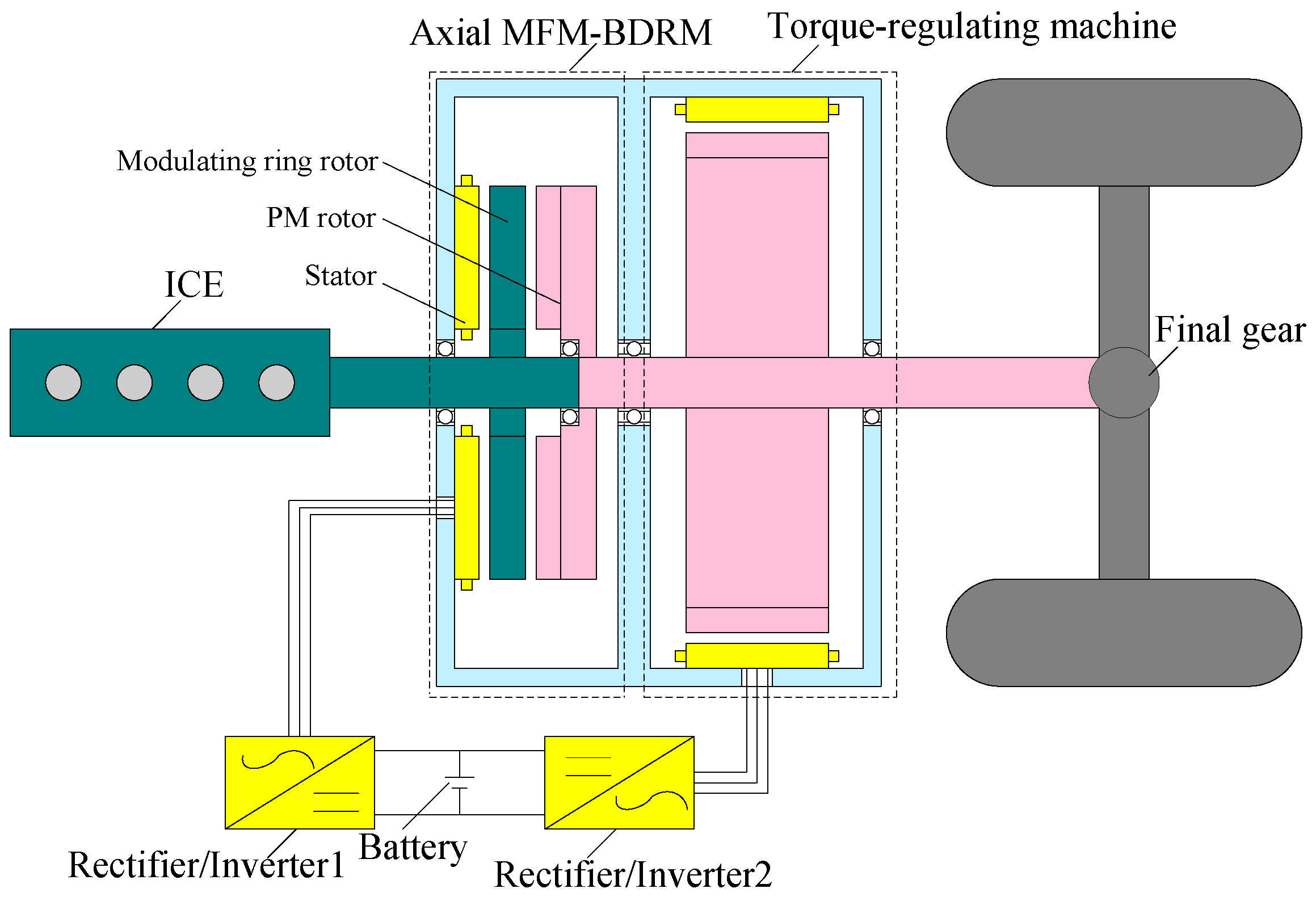
Analytical Investigation of the Magnetic-Field Distribution in an Axial Magnetic-Field-Modulated Brushless Double-Rotor Machine

Abstract

The axial magnetic-field-modulated brushless double-rotor machine (MFM-BDRM) is a novel possible alternative power-split device for hybrid electric vehicles (HEVs). This paper proposes a two-dimensional (2-D) analytical method to predict the performance of the axial MFM-BDRM to reduce computing time. The computation is based on the solution of Laplace’s or Poisson’s equation with boundary conditions for each elementary rectangular region. By taking account of the existence of modulating ring and the stator slotting effect, the proposed model is able to calculate magnetic-field distribution with high accuracy. In order to assess the proposed method, the 2-D analytical and three-dimensional (3-D) finite element analysis (FEA) results have been compared, and good agreements have been achieved. As the analytical computation is much faster and more flexible, the proposed method can be used in the preliminary design process of the axial MFM-BDRM.

1. Introduction

In recent years, double-rotor machines have drawn a wide interest as a possible alternative to the Toyota hybrid system (THS), which enables the internal combust engine (ICE) to operate at the high-efficiency area independent of road conditions [1,2,3,4]. However, the existence of brushes and slip rings may cause problems of low reliability and overheating of inner-rotor windings, which restricts their applications [5,6,7]. Therefore, a brushless double-rotor machine based on the principle of magnetic-field modulation, viz. magnetic-field-modulated brushless double-rotor machine (MFM-BDRM), has been proposed.

For a permanent magnet (PM) synchronous machine, axial-flux motors are capable of delivering high torque if the axial length is very short within a range of ratio R between admissible axial length and admissible diameter of 0.1–0.3, where the range of torque density is 3–6.5 Nm/kg. Radial-flux motors are attractive for long-shaft structures with a range of R between 1 and 2, where the range of torque density is 1.6–4 Nm/kg [8,9]. Compared with radial-flux topology of the MFM-BDRM, the axial-flux topology is superior in terms of high torque density and utilization of axial space, which has potential application prospect in hybrid electric vehicles (HEVs) [10,11,12,13,14,15].

The axial MFM-BDRM is composed of three parts: a stator, a modulating ring rotor and a PM rotor, as shown in Figure 1. The modulating ring rotor, which comprises ferromagnetic blocks (FBs) and nonmagnetic blocks (NBs) with even distribution, is sandwiched between the stator and the PM rotor. Different from conventional machines, the pole-pair number of the stator P_s is not equal to that of the PM rotor P_p, as a result of the existence of the modulating ring. The relationship of the P_s, P_p and the number of FBs P_f, is given by Equation (1):

$$P_{\mathrm{s}}+P_{\mathrm{p}}=P_{\mathrm{f}}$$

(1)

In previous research on the axial MFM-BDRM [16], the operating principle has been deduced. The rotational speed relationship of three parts is governed by Equation (2):

$$n_{\mathrm{s}}=\frac{n_{\mathrm{m}}{P}_{\mathrm{f}}-n_{\mathrm{p}}{P}_{\mathrm{p}}}{p_{\mathrm{s}}}$$

(2)

where n_m, n_p and n_s are the rotational speeds of modulating ring, PM rotor and stator magnetic field, respectively.

It can be seen from Equation (2) that the axial MFM-BDRM enables speed decoupling between two rotors by adjusting the stator current frequency. A scheme with P_s = 3, P_p = 20 and P_m = 23 is adopted to explain the operating principle in detail. For example, to obtain n_m = 1000 rpm and n_p = 700 rpm, n_s should be 3000 rpm, i.e., the frequency of stator current f_s = 150 Hz. If n_m is still 1000 rpm, n_p can be changed from 700 rpm to 1000 rpm by adjusting f_s from 150 Hz to 50 Hz.

The torque relationship of two rotors is governed by Equation (3):

$$\frac{T_{\mathrm{m}}}{T_{\mathrm{p}}}=-\frac{P_{\mathrm{f}}}{P_{\mathrm{p}}}$$

(3)

where T_m and T_p are the torques of modulating ring and PM rotor, respectively. It can be seen from Equation (3) that the machine can only transfer the torque with a fixed ratio.

Therefore, the axial MFM-BDRM connected with a torque-regulating machine can work as a power-split device in HEVs, as shown in Figure 2. To obtain the electromagnetic performance of the axial MFM-BDRM, such as no-load back electromotive force (EMF), torque and axial force, the prediction of air-gap magnetic-field distribution is required. Two types of method can be used for this calculation, i.e., analytical methods and numerical methods. Though numerical methods, like the three-dimensional (3-D) finite element method (FEM), offer accurate results by taking into account the real geometry and the magnetic saturation of the iron parts, they are time-consuming and less flexible for the initial design procedure. Analytical methods predict the magnetic-field distribution with assumptions like simplified geometry and unsaturated iron, which enables an acceptable compromise between compution time and accuracy. Moreover, given the fact that numerous optimizations of geometrical parameters are possible for the axial MFM-BDRM, an analytical method with low computing time can be an effective tool for the first step of design optimization to determine initial scheme before accurate optimization with 3-D FEM.

Many analytical methods have been proposed for the PM machines without taking into account the slotting effect, and generally focus on the open-circuit field distribution. In [17,18,19,20], the stator slotting effect on the magnetic-field distribution is considered, which is critical for the accurate calculation of the cogging torque and PM eddy losses, etc. In [21,22,23,24], a 2-D analytical model has been proposed for the magnetic gear, where the modulation effect on the magnetic-field distribution can be evaluated. For the axial MFM-BDRM, magnetic-field distribution is more complicated with the co-existence of the stator slots and the modulating ring. However, few studies have been done on the performance prediction of the axial MFM-BDRM by analytical methods. In this paper, a 2-D analytical method to predict the performance of the axial-flux magnetic-geared machine is proposed. Special attention is paid on the precise calculation of the open-circuit and armature reaction field distribution in consideration of the modulation and stator slot-opening effect. Hence, performances of the machine such as no-load back EMF, torque and axial force, can be predicted with acceptable calculation time and accuracy. In order to evaluate the proposed method, the analytical predictions are compared with 3-D FEM simulations.

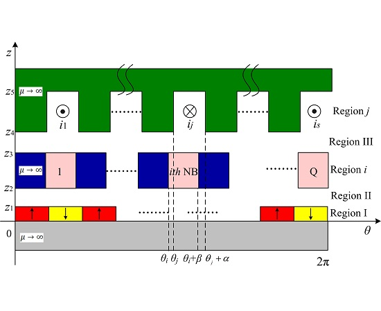
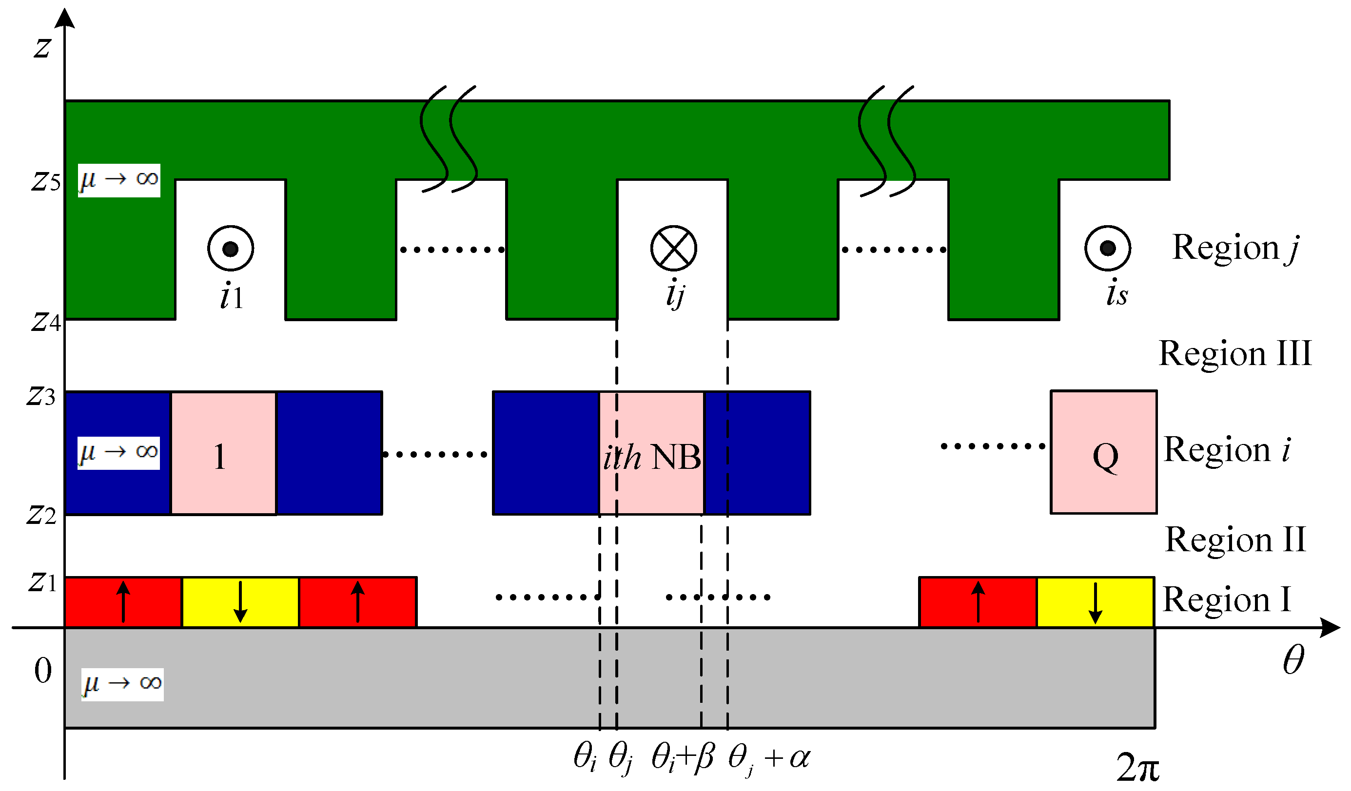
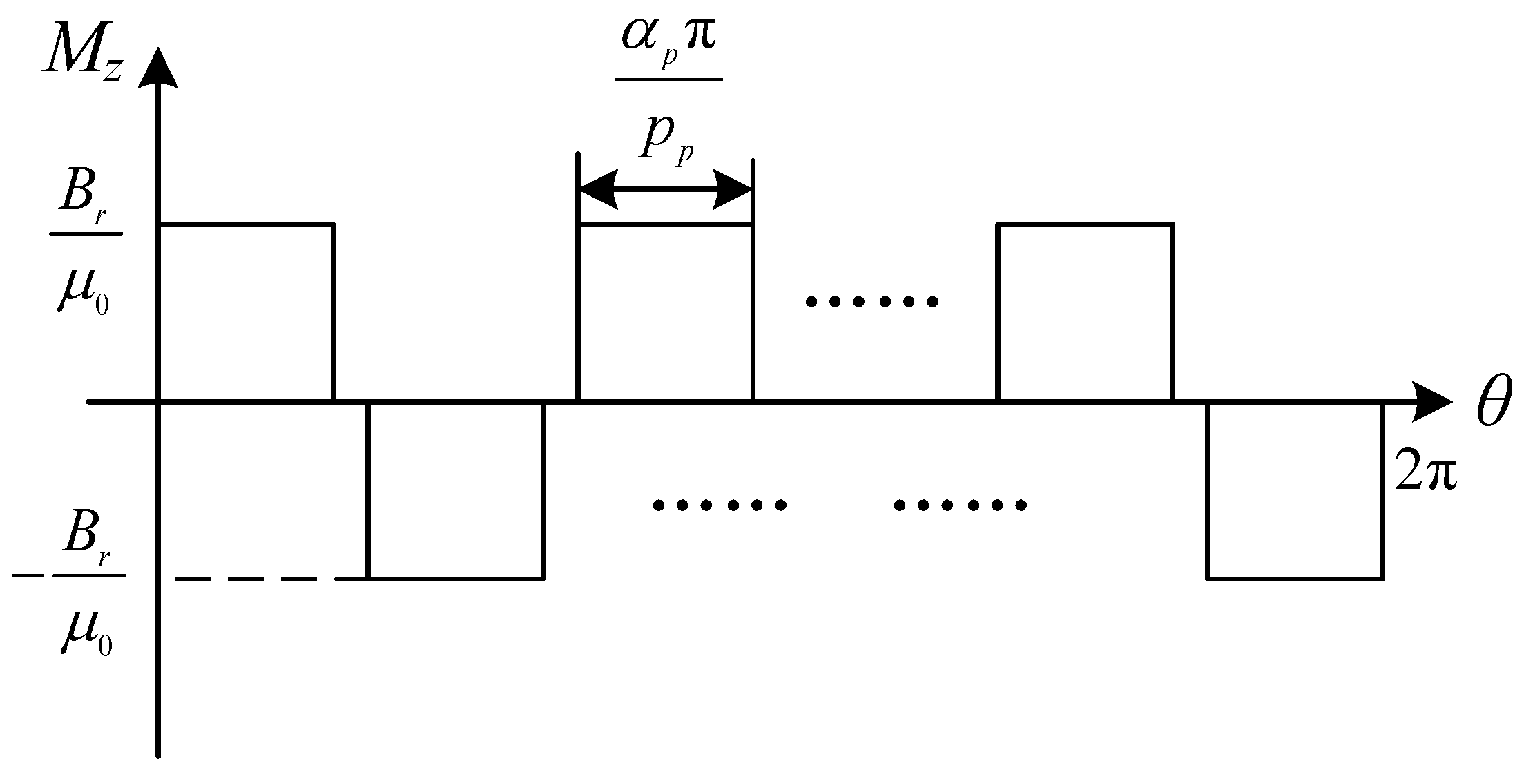
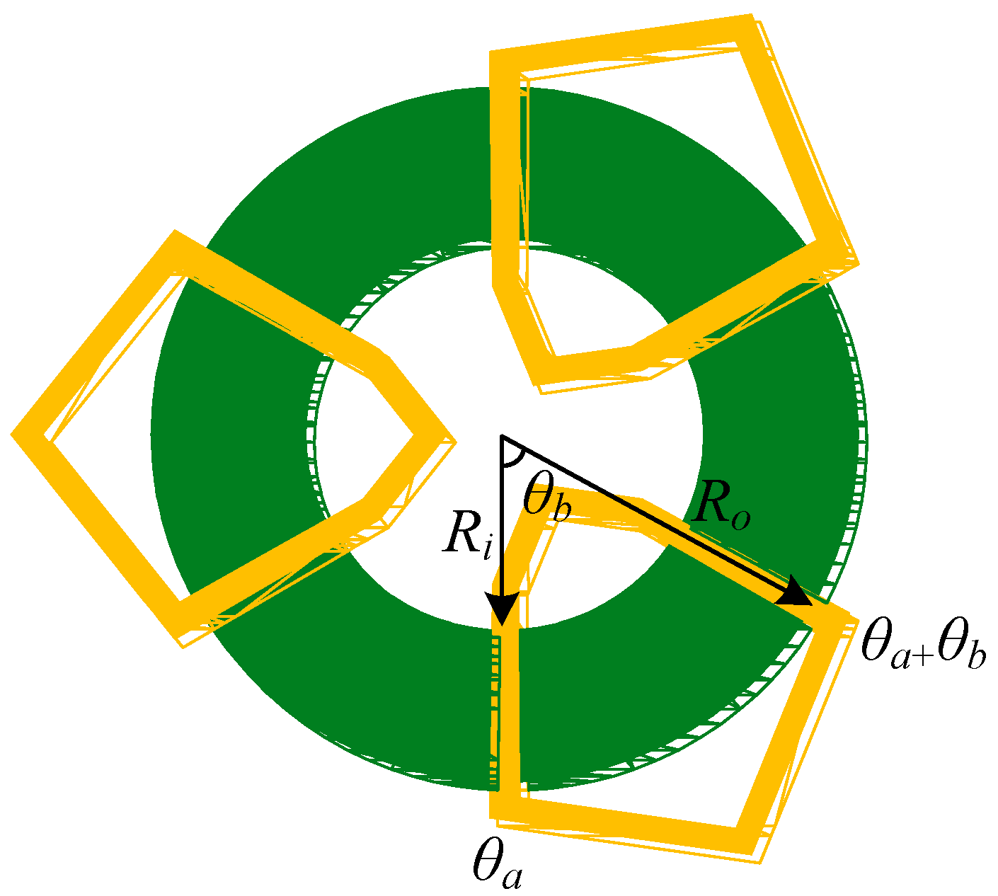
2. Analytical Modeling

Analytical study of the axial MFM-BDRM is complicated due to the 3-D distribution of the magnetic field. In order to simplify the analysis, the 3-D problem is converted to a 2-D one by introducing a cylindrical section at the mean radius of the axial MFM-BDRM at which the magnetic field will be calculated.

Figure 3 shows the 2-D analytical model of unrolled cylindrical section, in which z₁, (z₂ − z₁), (z₃ − z₂), (z₄ − z₃) and (z₅ − z₄) are the thickness of PM, inner air gap, NB, outer air gap and stator slot, respectively. β is the NB angle and Q is the pole number of NB. α is the slot angle and S is the slot number. θ_i and θ_j are the angular position of the i-th NB and j-th stator slot, which can be defined as:

$${\mathsf{\theta }}_i=\frac{2\mathsf{\pi }(i-1)}{Q}+{\mathsf{\theta }}_{\mathrm{n}0}$$

(4)

$${\mathsf{\theta }}_j=\frac{2\mathsf{\pi }(j-1)}{S}+{\mathsf{\theta }}_{\mathrm{s}0}$$

(5)

where θ_n0 and θ_s0 are the initial angular positions of the NB and stator slot, respectively.

For simplicity, the following assumptions are adopted:

(1)

The soft-magnetic material (iron) has infinite magnetic permeability μ → ∞;

(2)

The PMs are axially magnetized with relative permeability μ_r = 1.

Therefore, the analytical model can be divided into five regions: the PM region (I), the air-gap regions (II and III), the NB regions (i) and the stator slot region (j). Magnetic-field distribution in two air gaps can be solved based on Laplace’s or Poisson’s equation with corresponding boundary conditions in each region.

3. Analytical Solution

3.1. Governing Partial Differential Equations

Magnetic vector potential A is introduced here to describe the field behavior. The governing partial differential equation in each region can be expressed in Equation (6):

$$\{\begin{array}{cc}{\nabla }^2\mathit{A}=0\hfill & \mathrm{in}\hspace{0.17em}\mathrm{Region}\hspace{0.17em}\mathrm{II}, \mathrm{III}, i\hfill \\ {\nabla }^2\mathit{A}=-{\mathsf{\mu }}_0\mathit{J}\hfill & \mathrm{in}\hspace{0.17em}\mathrm{Region} j\hfill \\ {\nabla }^2\mathit{A}=-{\mathsf{\mu }}_0\nabla \times \mathit{M}\hfill & \mathrm{in}\hspace{0.17em}\mathrm{Region}\hspace{0.17em}\hspace{0.17em}\mathrm{I}\hfill \end{array}$$

(6)

with:

$$\mathit{M}=\pm \frac{B_r}{{\mathsf{\mu }}_0}{\mathit{e}}_z$$

(7)

where J is the armature current density vector, M is the magnetization vector and B_r is the remanence of the magnets. By using the Cartesian coordinates (y, z) and replacing y by R_mθ, Equation (6) can be rewritten as:

$$\frac{1}{R_{\mathrm{m}}^2}\frac{{\partial }^2{A}_I}{\partial {\mathsf{\theta }}^2}+\frac{{\partial }^2{A}_I}{\partial z^2}=-\frac{{\mathsf{\mu }}_0}{R_{\mathrm{m}}}\frac{\partial M_z}{\partial \mathsf{\theta }} \{\begin{array}{l}0\le z\le z_1\\ 0\le \mathsf{\theta }\le 2\mathsf{\pi }\end{array}$$

(8)

$$\frac{1}{R_{\mathrm{m}}^2}\frac{{\partial }^2{A}_{II}}{\partial {\mathsf{\theta }}^2}+\frac{{\partial }^2{A}_{II}}{\partial z^2}=0 \{\begin{array}{l}{z}_1\le z\le z_2\\ 0\le \mathsf{\theta }\le 2\mathsf{\pi }\end{array}$$

(9)

$$\frac{1}{R_{\mathrm{m}}^2}\frac{{\partial }^2{A}_i}{\partial {\mathsf{\theta }}^2}+\frac{{\partial }^2{A}_i}{\partial z^2}=0 \{\begin{array}{l}{z}_2\le z\le z_3\\ {\mathsf{\theta }}_i\le \mathsf{\theta }\le {\mathsf{\theta }}_i+\mathsf{\beta }\hspace{0.17em}\end{array}$$

(10)

$$\frac{1}{R_{\mathrm{m}}^2}\frac{{\partial }^2{A}_{\mathrm{III}}}{\partial {\mathsf{\theta }}^2}+\frac{{\partial }^2{A}_{\mathrm{III}}}{\partial z^2}=0 \{\begin{array}{l}{z}_3\le z\le z_4\\ 0\le \mathsf{\theta }\le 2\mathsf{\pi }\end{array}$$

(11)

$$\frac{1}{R_m^2}\frac{{\partial }^2{A}_j}{\partial {\mathsf{\theta }}^2}+\frac{{\partial }^2{A}_j}{\partial z^2}=-{\mathsf{\mu }}_0{J}_s^j \{\begin{array}{l}{z}_4\le z\le z_5\\ {\mathsf{\theta }}_j\le \mathsf{\theta }\le {\mathsf{\theta }}_j+\mathsf{\alpha }\end{array}$$

(12)

where R_m is the mean radius of the machine; A_I, A_II, A_i, A_III and A_j are the magnetic vector potentials in the PM, inner air-gap, NB, outer air-gap and stator slot regions, respectively; J_s^j is the armature current density of the j-th stator slot; M_z is the axial magnetization of the PM. The distribution of the axial magnetization M_z is shown in Figure 4. Therefore, the axial magnetization can be expressed in Fourier’s series:

$$M_z(\mathsf{\theta })={\displaystyle \sum _{n=1}^{\infty }\frac{4B_r}{(2n-1)\mathsf{\pi }{\mathsf{\mu }}_0}}\cos ((2n-1)\frac{\mathsf{\pi }}{2}(1-{\mathsf{\alpha }}_{\mathrm{p}}))\sin ((2n-1)P_{\mathrm{p}}(\mathsf{\theta }-{\mathsf{\theta }}_{\mathrm{p}0}))\hspace{0.17em}\hspace{0.17em}\hspace{0.17em}\hspace{0.17em}\hspace{0.17em}\hspace{0.17em}\mathrm{with}\hspace{0.17em}n=1,2,3,\mathrm{4...}$$

(13)

where θ_p0 is the initial phase angle of the PM and α_p is the pole-arc coefficient of the PM rotor.

Distributed full-pitch winding with one slot per pole per phase is adopted for the investigated machine. Figure 5 shows a distributed current sheet representation of three-phase stator winding, which is accommodated in slots. Therefore, the current density can be expressed as:

$$J_{\mathrm{s}}^j=\frac{I_{\mathrm{m}}{N}_t\cos ({\mathsf{\theta }}_{\mathrm{sp}0}-\frac{\mathsf{\pi }}{3}(j-1))}{h_{\mathrm{s}}{w}_{\mathrm{s}}}\hspace{0.17em}\hspace{0.17em}\hspace{0.17em}\hspace{0.17em},\hspace{0.17em}\hspace{0.17em}1\le j\le S$$

(14)

where I_m is the amplitude of one-phase current; N_t is the number of conductors per slot; θ_sp0 is the initial phase angle of current in the first slot; h_s and w_s are the height and width of the slot, respectively.

3.2. Boundary Conditions

At the interface between two adjacent media, the magnetic vector potential is continuous. If the interface is source-free, the tangential component of the magnetic field intensity on one side of the boundary is equal to that of the other side. Therefore, the boundary conditions of the axial MFM-BDRM can be listed as below.

3.2.1. At the Interface z = 0

The tangential component of the magnetic field intensity on the PM side is null as the yoke of the PM rotor has infinite magnetic permeability:

$${\frac{1}{{\mathsf{\mu }}_0}\frac{\partial A_{\mathrm{I}}}{\partial z}|}_{z=0}=0$$

(15)

3.2.2. At the Interface z = z₁

The magnetic vector potential is continuous:

$$A_I(\mathsf{\theta },z_1)=A_{\mathrm{II}}(\mathsf{\theta },z_1)$$

(16)

The tangential component of magnetic field intensity is continuous:

$${\frac{1}{{\mathsf{\mu }}_0}\frac{\partial A_{II}}{\partial z}|}_{z=z_1}=\frac{1}{{\mathsf{\mu }}_0}{\frac{\partial A_I}{\partial z}|}_{z=z_1}$$

(17)

3.2.3. At the Interface z = z₂

The tangential component of magnetic field intensity is continuous on the boundary between the inner air gap and each NB while it is null on the boundary between the inner air gap and each FB:

$$\frac{1}{{\mathsf{\mu }}_0}{\frac{\partial A_{II}}{\partial z}|}_{z=z_2}=\{\begin{array}{ccc}{\frac{1}{{\mathsf{\mu }}_0}\frac{\partial A_i}{\partial z}|}_{z=z_2}\hfill & \hfill ,\hfill & \hfill \forall {\mathsf{\theta }}_i\le \mathsf{\theta }\le {\mathsf{\theta }}_i+\mathsf{\beta }\hfill \\ 0\hfill & \hfill ,\hfill & \hfill \mathrm{elsewhere}\hfill \end{array}$$

(18)

The magnetic vector potential is continuous on the boundary between the inner air gap and each NB:

$$A_i(\mathsf{\theta },z_2)=A_{\mathrm{II}}(\mathsf{\theta },z_2)\hspace{0.17em}\hspace{0.17em}\hspace{0.17em}\hspace{0.17em}\hspace{0.17em}\hspace{0.17em}\hspace{0.17em}\hspace{0.17em}\forall {\mathsf{\theta }}_i\le \mathsf{\theta }\le {\mathsf{\theta }}_i+\mathsf{\beta }$$

(19)

3.2.4. At the Interface z = z₃

The tangential component of magnetic field intensity is continuous on the boundary between the outer air gap and each NB while it is null on the boundary between the outer air gap and each FB:

$${\frac{1}{{\mathsf{\mu }}_0}\frac{\partial A_{III}}{\partial z}|}_{z=z_3}=\{\begin{array}{ccc}{\frac{1}{{\mathsf{\mu }}_0}\frac{\partial A_i}{\partial z}|}_{z=z_3}\hfill & \hfill ,\hfill & \hfill \forall {\mathsf{\theta }}_i\le \mathsf{\theta }\le {\mathsf{\theta }}_i+\mathsf{\beta }\\ 0\hfill & \hfill ,\hfill & \hfill \mathrm{elsewhere}\end{array}$$

(20)

The magnetic vector potential is continuous on the boundary between the outer air gap and each NB:

$$A_i(\mathsf{\theta },z_3)=A_{\mathrm{III}}(\mathsf{\theta },z_3)\hspace{0.17em}\hspace{0.17em}\hspace{0.17em}\hspace{0.17em}\hspace{0.17em}\hspace{0.17em}\hspace{0.17em}\hspace{0.17em}\forall {\mathsf{\theta }}_i\le \mathsf{\theta }\le {\mathsf{\theta }}_i+\mathsf{\beta }$$

(21)

3.2.5. At the Interface z = z₄

The tangential component of magnetic field intensity is continuous on the boundary between the outer air gap and each stator slot while it is null on the boundary between the outer air gap and each stator tooth:

$$\frac{1}{{\mathsf{\mu }}_0}{\frac{\partial A_{III}}{\partial z}|}_{z=z_4}=\{\begin{array}{ccc}{\frac{1}{{\mathsf{\mu }}_0}\frac{\partial A_j}{\partial z}|}_{z=z_4}\hfill & \hfill ,\hfill & \hfill \forall {\mathsf{\theta }}_j\le \mathsf{\theta }\le {\mathsf{\theta }}_j+\mathsf{\alpha }\hfill \\ 0\hfill & \hfill ,\hfill & \hfill \mathrm{elsewhere}\hfill \end{array}$$

(22)

The magnetic vector potential is continuous on the boundary between the outer air gap and each stator slot:

$$A_j(\mathsf{\theta },z_4)=A_{\mathrm{III}}(\mathsf{\theta },z_4)\hspace{0.17em}\hspace{0.17em}\hspace{0.17em}\hspace{0.17em}\hspace{0.17em}\hspace{0.17em}\hspace{0.17em}\hspace{0.17em}\forall {\mathsf{\theta }}_j\le \mathsf{\theta }\le {\mathsf{\theta }}_j+\mathsf{\alpha }$$

(23)

3.2.6. At the Interface z = z₅

The tangential component of the magnetic field intensity on the stator slot side is null:

$${\frac{1}{{\mathsf{\mu }}_0}\frac{\partial A_j}{\partial z}|}_{z=z_5}=0$$

(24)

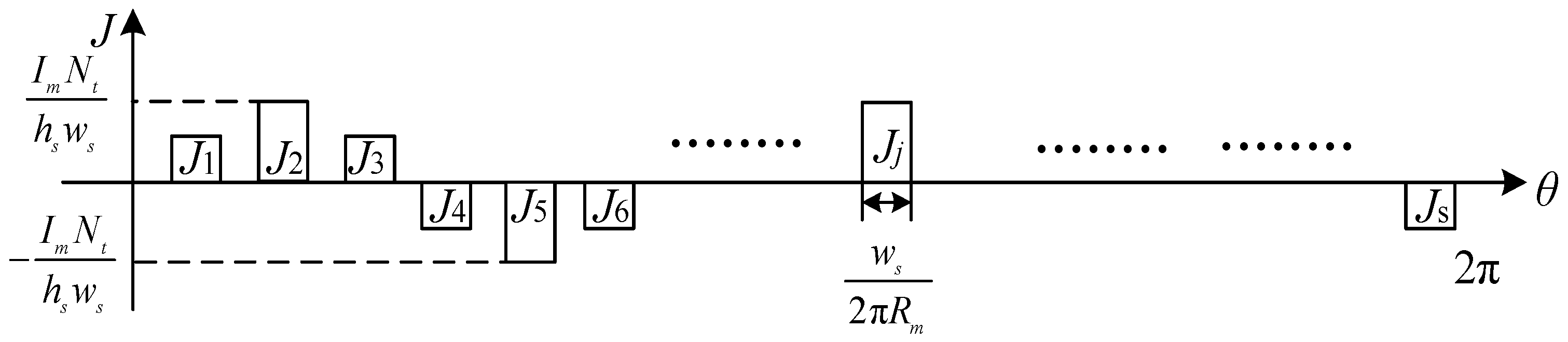
3.2.7. At the Interface θ = θ_i and θ = θ_i + β

The tangential component of magnetic field intensity is null at both sides of the each NB:

$${-\frac{1}{{\mathsf{\mu }}_0{R}_{\mathrm{m}}}\frac{\partial A_i}{\partial \mathsf{\theta }}|}_{\mathsf{\theta }=\mathsf{\theta }{}_i}=-\frac{1}{{\mathsf{\mu }}_0{R}_{\mathrm{m}}}{\frac{\partial A_i}{\partial \mathsf{\theta }}|}_{\mathsf{\theta }=\mathsf{\theta }{}_i+\mathsf{\beta }}=0$$

(25)

3.2.8. At the Interface θ = θ_j and θ = θ_j + α

The tangential component of magnetic field intensity is null at both sides of the each stator slot is null:

$${-\frac{1}{{\mathsf{\mu }}_0{R}_{\mathrm{m}}}\frac{\partial A_j}{\partial \mathsf{\theta }}|}_{\mathsf{\theta }=\mathsf{\theta }{}_j}=-\frac{1}{{\mathsf{\mu }}_0{R}_{\mathrm{m}}}{\frac{\partial A_j}{\partial \mathsf{\theta }}|}_{\mathsf{\theta }=\mathsf{\theta }{}_j+\mathsf{\alpha }}=0$$

(26)

3.3. General Solutions

From Equations (8) and (15), the general solution of the magnetic vector potential in the PM region is:

$$A_{\mathrm{I}}(\mathsf{\theta },z)={\displaystyle \sum _{n=1}^{\infty }(a_n^I\frac{ch(\frac{n}{R_{\mathrm{m}}}z)}{ch(\frac{n}{R_{\mathrm{m}}}{z}_1)}+K_n^{\mathrm{h}}\cos (n{\mathsf{\delta }}_{\mathrm{h}}))\cos (n\mathsf{\theta })}+{\displaystyle \sum _{n=1}^{\infty }(c_n^{\mathrm{I}}\frac{ch(\frac{n}{R_{\mathrm{m}}}z)}{ch(\frac{n}{R_{\mathrm{m}}}{z}_1)}+K_n^{\mathrm{h}}\sin (n{\mathsf{\delta }}_{\mathrm{h}}))\sin (n\mathsf{\theta })}$$

(27)

with:

$$K_n^{\mathrm{h}}=\{\begin{array}{cc}\frac{4B_{\mathrm{r}}{R}_{\mathrm{m}}{P}_p}{\mathsf{\pi }{n}^2}\cos (n\frac{\mathsf{\pi }}{2P_{\mathrm{p}}}(1-{\mathsf{\alpha }}_{\mathrm{p}}))\hfill & \mathrm{for}\hspace{0.17em}\hspace{0.17em}n=j{P}_{\mathrm{p}};\hspace{0.17em}j=1,\hspace{0.17em}3,\hspace{0.17em}5\hspace{0.17em}\mathrm{......}\hfill \\ 0\hfill & \mathrm{otherwise}\hfill \end{array}$$

(28)

From Equation (9), the general solution of the magnetic vector potential in the inner air-gap region is:

$$\begin{array}{cc}{A}_{\mathrm{II}}(\mathsf{\theta },z)\hfill & ={\displaystyle \sum _{n=1}^{\infty }(a_n^{\mathrm{II}}\frac{R_{\mathrm{m}}}{n}\frac{ch(\frac{n}{R_{\mathrm{m}}}(z-z_2))}{sh(\frac{n}{R_{\mathrm{m}}}(z_1-z_2))}+b_n^{\mathrm{II}}\frac{R_{\mathrm{m}}}{n}\frac{ch(\frac{n}{R_{\mathrm{m}}}(z-z_1))}{sh(\frac{n}{R_{\mathrm{m}}}(z_2-z_1))})\cos (n\mathsf{\theta })}\hfill \\ & +{\displaystyle \sum _{n=1}^{\infty }(c_n^{\mathrm{II}}\frac{R_{\mathrm{m}}}{n}\frac{ch(\frac{n}{R_{\mathrm{m}}}(z-z_2))}{sh(\frac{n}{R_{\mathrm{m}}}(z_1-z_2))}+d_n^{\mathrm{II}}\frac{R_{\mathrm{m}}}{n}\frac{ch(\frac{n}{R_{\mathrm{m}}}(z-z_1))}{sh(\frac{n}{R_{\mathrm{m}}}(z_2-z_1))})\sin (n\mathsf{\theta })}\hfill \end{array}$$

(29)

From Equations (10) and (25), the general solution of the magnetic vector potential in the i-th NB region is:

$$A_i(\mathsf{\theta },z)=a_0^i+b_0^{i}z+{\displaystyle \sum _{k=1}^{\infty }(a_k^i\frac{sh(\frac{k\mathsf{\pi }}{\mathsf{\beta }{R}_{\mathrm{m}}}(z-z_3))}{sh(\frac{k\mathsf{\pi }}{\mathsf{\beta }{R}_{\mathrm{m}}}(z_2-z_3))}+b_k^i\frac{sh(\frac{k\mathsf{\pi }}{\mathsf{\beta }{R}_{\mathrm{m}}}(z-z_2))}{sh(\frac{k\mathsf{\pi }}{\mathsf{\beta }{R}_{\mathrm{m}}}(z_3-z_2))})\cos (\frac{k\mathsf{\pi }}{\mathsf{\beta }}(\mathsf{\theta }-{\mathsf{\theta }}_i))}$$

(30)

From Equation (11), the general solution of the magnetic vector potential in the outer air-gap region is:

$$\begin{array}{cc}{A}_{\mathrm{III}}(\mathsf{\theta },z)\hfill & ={\displaystyle \sum _{n=1}^{\infty }(a_n^{\mathrm{III}}\frac{R_{\mathrm{m}}}{n}\frac{ch(\frac{n}{R_{\mathrm{m}}}(z-z_3))}{sh(\frac{n}{R_{\mathrm{m}}}(z_4-z_3))}+b_n^{\mathrm{III}}\frac{R_{\mathrm{m}}}{n}\frac{ch(\frac{n}{R_{\mathrm{m}}}(z-z_4))}{sh(\frac{n}{R_{\mathrm{m}}}(z_3-z_4))})\cos (n\mathsf{\theta })}\hfill \\ & +{\displaystyle \sum _{n=1}^{\infty }(c_n^{\mathrm{III}}\frac{R_{\mathrm{m}}}{n}\frac{ch(\frac{n}{R_{\mathrm{m}}}(z-z_3))}{sh(\frac{n}{R_{\mathrm{m}}}(z_4-z_3))}+d_n^{\mathrm{III}}\frac{R_{\mathrm{m}}}{n}\frac{ch(\frac{n}{R_{\mathrm{m}}}(z-z_4))}{sh(\frac{n}{R_{\mathrm{m}}}(z_3-z_4))})\sin (n\mathsf{\theta })}\hfill \end{array}$$

(31)

From Equations (12), (24) and (26), the general solution of the magnetic vector potential in the j-th stator slot region is:

$$A_j(\mathsf{\theta },z)=a_0^j+{\displaystyle \sum _{k=1}^{\infty }{a}_k^j\frac{ch(\frac{k\mathsf{\pi }}{\mathsf{\alpha }{R}_{\mathrm{m}}}(z-z_5))}{ch(\frac{k\mathsf{\pi }}{\mathsf{\alpha }{R}_{\mathrm{m}}}(z_4-z_5))}\cos (\frac{k\mathsf{\pi }}{\mathsf{\alpha }}(\mathsf{\theta }-{\mathsf{\theta }}_j))}-\frac{1}{2}{\mathsf{\mu }}_0{J}_{\mathrm{s}}^j{(z-z_5)}^2$$

(32)

3.4. Magnetic-Field Distribution in Two Air Gaps

The axial and tangential components of the magnetic flux density in the inner air-gap region can be expressed as:

$$B_{\mathrm{zII}}=-\frac{1}{R_{\mathrm{m}}}\frac{\partial A_{\mathrm{II}}}{\partial \mathsf{\theta }}\hspace{0.17em}\hspace{0.17em}\hspace{0.17em}\hspace{0.17em}\hspace{0.17em}\hspace{0.17em}\hspace{0.17em}\hspace{0.17em}\hspace{0.17em}\hspace{0.17em}\hspace{0.17em}\hspace{0.17em}\hspace{0.17em}\hspace{0.17em}\hspace{0.17em}{B}_{\mathsf{\theta }\mathrm{II}}=\frac{\partial A_{\mathrm{II}}}{\partial z}$$

(33)

The axial and tangential components of the magnetic flux density in the outer air-gap region can be expressed as:

$$B_{\mathrm{zIII}}=-\frac{1}{R_{\mathrm{m}}}\frac{\partial A_{\mathrm{III}}}{\partial \mathsf{\theta }}\hspace{0.17em}\hspace{0.17em}\hspace{0.17em}\hspace{0.17em}\hspace{0.17em}\hspace{0.17em}\hspace{0.17em}\hspace{0.17em}\hspace{0.17em}\hspace{0.17em}\hspace{0.17em}\hspace{0.17em}\hspace{0.17em}\hspace{0.17em}\hspace{0.17em}{B}_{\mathsf{\theta }\mathrm{II}}=\frac{\partial A_{\mathrm{III}}}{\partial z}$$

(34)

3.5. No-Load Back Electromotive Force

The layout of one-phase winding of the axial MFM-BDRM is shown in Figure 6, where R_i and R_o are the inner and outer radius, respectively. θ_a is the initial position angle of the a-th coil and θ_b is the span angle of two active sides of a coil.

Under the open-circuit condition, i.e., J = 0, one-phase flux linkage ψ_ph can be obtained from the integration of the outer air-gap flux density distribution adjacent to one phase, in which the outer air-gap flux density is represented by the magnetic-field distribution at the mean radius. As distributed full-pitch winding with one slot per pole per phase is adopted for the investigated machine, the number of coils per phase is P_s. One-phase flux linkage ψ_ph can be expressed as:

$${\mathsf{\psi }}_{\mathrm{ph}}={\displaystyle \sum _{a=1}^{P_{\mathrm{S}}}{N}_t{\displaystyle \underset{{\mathsf{\theta }}_a}{\overset{{\mathsf{\theta }}_a+{\mathsf{\theta }}_b}{\int }}{B}_{\mathrm{zIII}}\mathrm{d}\mathsf{\theta }}}\times \frac{(R_0^2-R_i^2)}{2}$$

(35)

Therefore, no-load back EMF can be achieved:

$$e_0(t)=-\frac{\mathrm{d}{\mathsf{\psi }}_{\mathrm{ph}}}{\mathrm{d}t}=-\frac{\mathrm{d}({\displaystyle \sum _{a=1}^{P_{\mathrm{S}}}{N}_t{\displaystyle \underset{{\mathsf{\theta }}_a}{\overset{{\mathsf{\theta }}_a+{\mathsf{\theta }}_b}{\int }}{B}_{\mathrm{zIII}}\mathrm{d}\mathsf{\theta }}}\times \frac{(R_0^2-R_i^2)}{2})}{\mathrm{d}t}\times \frac{(R_0^2-R_i^2)}{2}$$

(36)

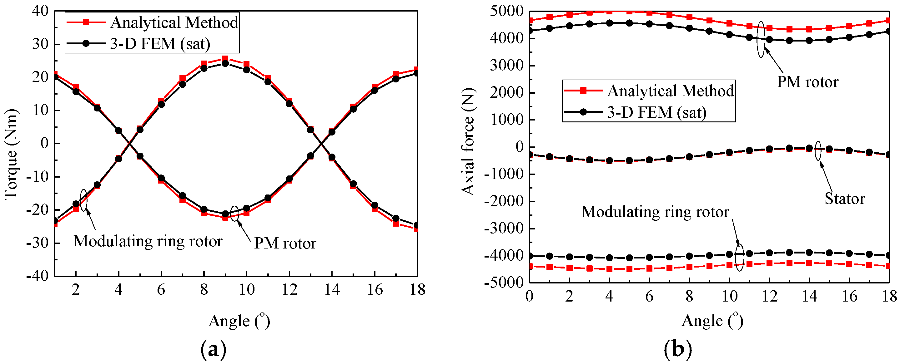
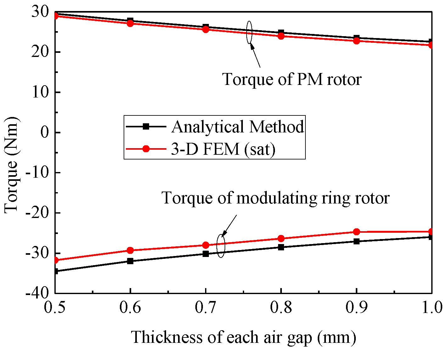
3.6. Torque and Axial Force

Based on the classical Maxwell stress tensor, torque and axial force on the PM rotor can be obtained as:

$$T_{\mathrm{p}}=\frac{(R_{\mathrm{o}}^2-R_{\mathrm{i}}^2)(R_{\mathrm{o}}+R_{\mathrm{i}})}{4{\mathsf{\mu }}_0}{\displaystyle \underset{0}{\overset{2\mathsf{\pi }}{\int }}{B}_{\mathrm{zII}}{B}_{\mathsf{\theta }\mathrm{II}}\mathrm{d}\mathsf{\theta }}$$

(37)

$$F_{\mathrm{p}}=\frac{(R_{\mathrm{o}}^2-R_{\mathrm{i}}^2)}{4{\mathsf{\mu }}_0}{\displaystyle \underset{0}{\overset{2\pi }{\int }}(B_{\mathrm{zII}}^2-B_{\mathsf{\theta }\mathrm{II}}^2)\mathrm{d}\mathsf{\theta }}$$

(38)

Similarly, torque and axial force on the stator can be obtained. Therefore, torque and axial force on the modulating ring is:

$$T_{\mathrm{m}}=-(T_{\mathrm{s}}+T_{\mathrm{p}})$$

(39)

$$F_{\mathrm{m}}=-(F_{\mathrm{s}}+F_{\mathrm{p}})$$

(40)

4. Analytical Method Evaluation

In order to evaluate the accuracy of the proposed method, the analytical results are compared with 3-D FEM results. The geometrical parameters are listed in

Table 1. Parameters of the investigated machine. FB: ferromagnetic block.

Symbol	Quantity	Value
Ri	inner radius	64 mm
Ro	outer radius	114 mm
z1	PM thickness	4 mm
z2 − z1	inner air-gap thickness	1 mm
z3 − z2	FB thickness	11 mm
z4 − z3	outer air-gap thickness	1 mm
Q	pole number of FB	23
pp	pole-pair number of PM rotor	20
ps	pole-pair number of stator	3
S	slot number	18
hs	height of slot	11 mm
ws	width of slot	19.3 mm
αp	pole-arc coefficient of PM rotor	1
αf	arc ratio of FB	0.5
Nt	number of conductors per slot	13
wt	width of tooth at the mean radius	11.8 mm
Br	Remanent flux density of PM	1.26 T
I	Root mean square value of one-phase current	30 A

.

The 3-D finite element simulations are carried out by using the software of Cedrat Flux. The 3-D model is shown in Figure 1a, in which the long sheet steel is rolled up for the stator core and cut with slots. Axially magnetized NdFeB PMs are mounted on the surface of PM rotor, whose core also adopts sheet steel with rolled lamination. Sheet steel with radial lamination is used for the FB and epoxy resin is employed for the NB.

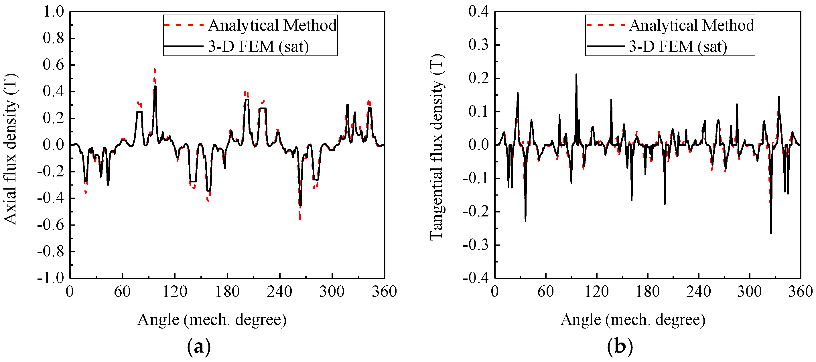
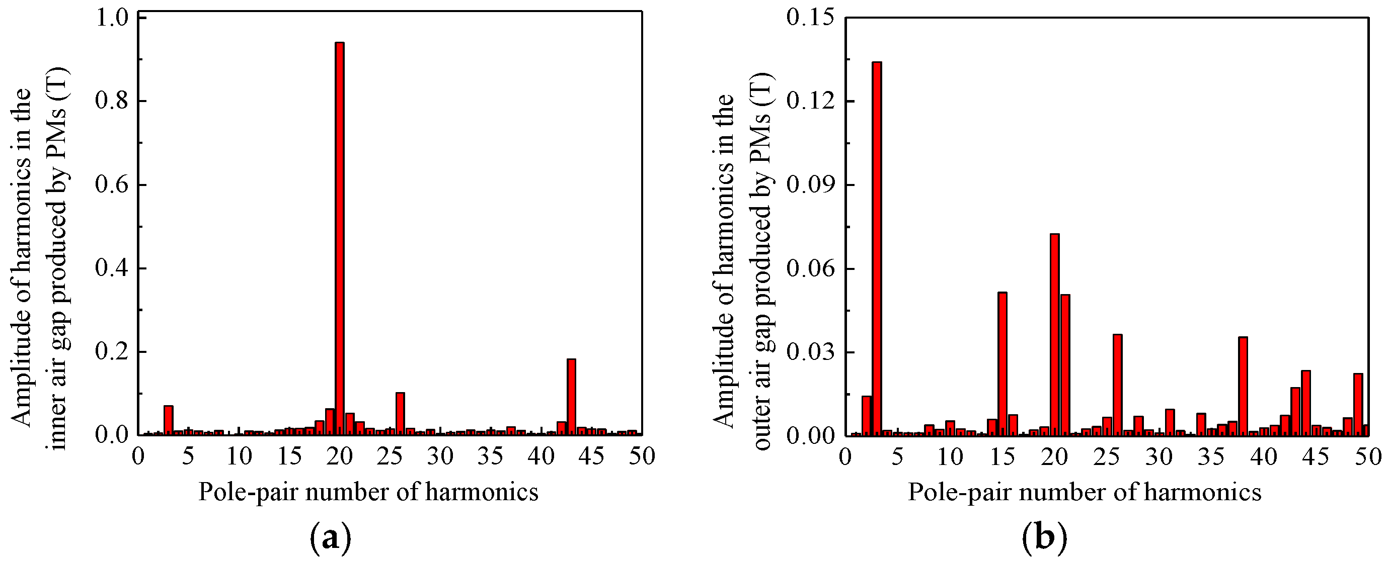
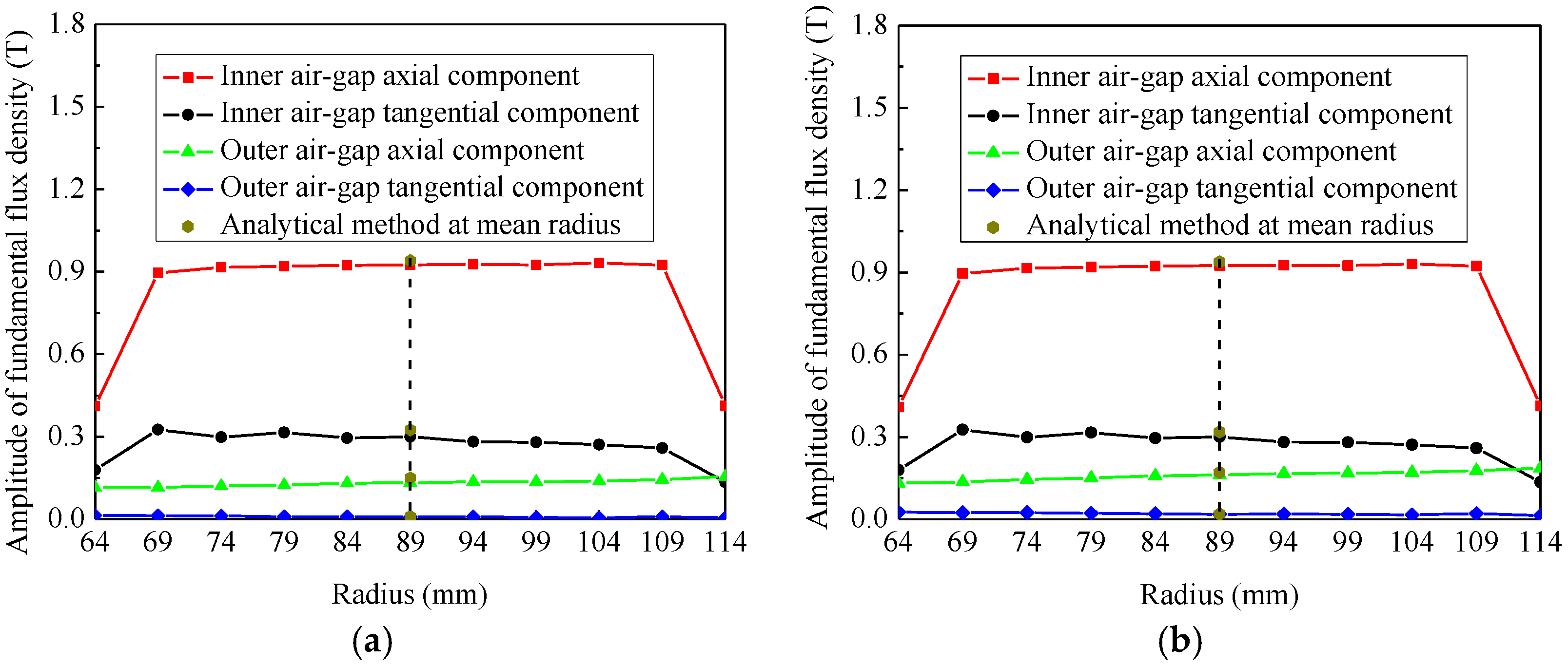
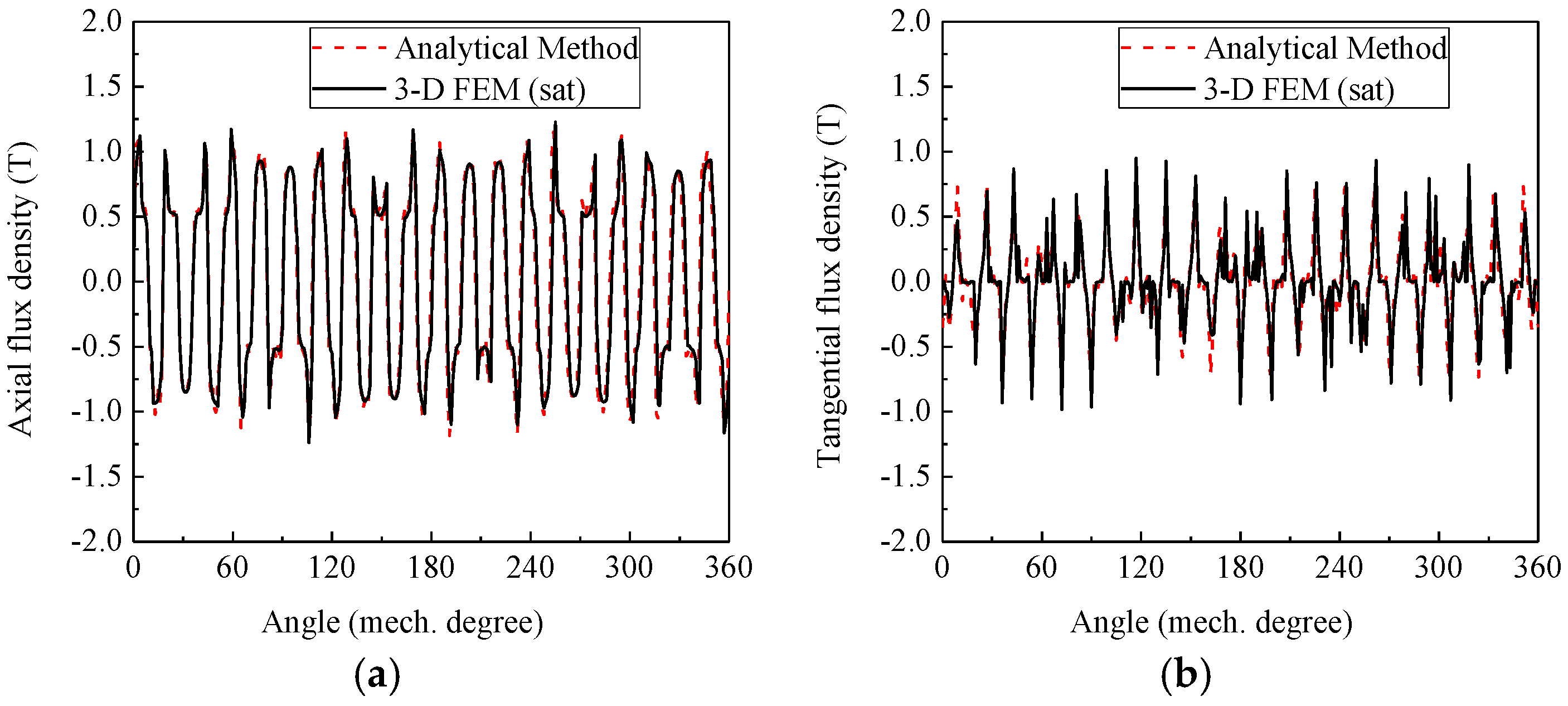
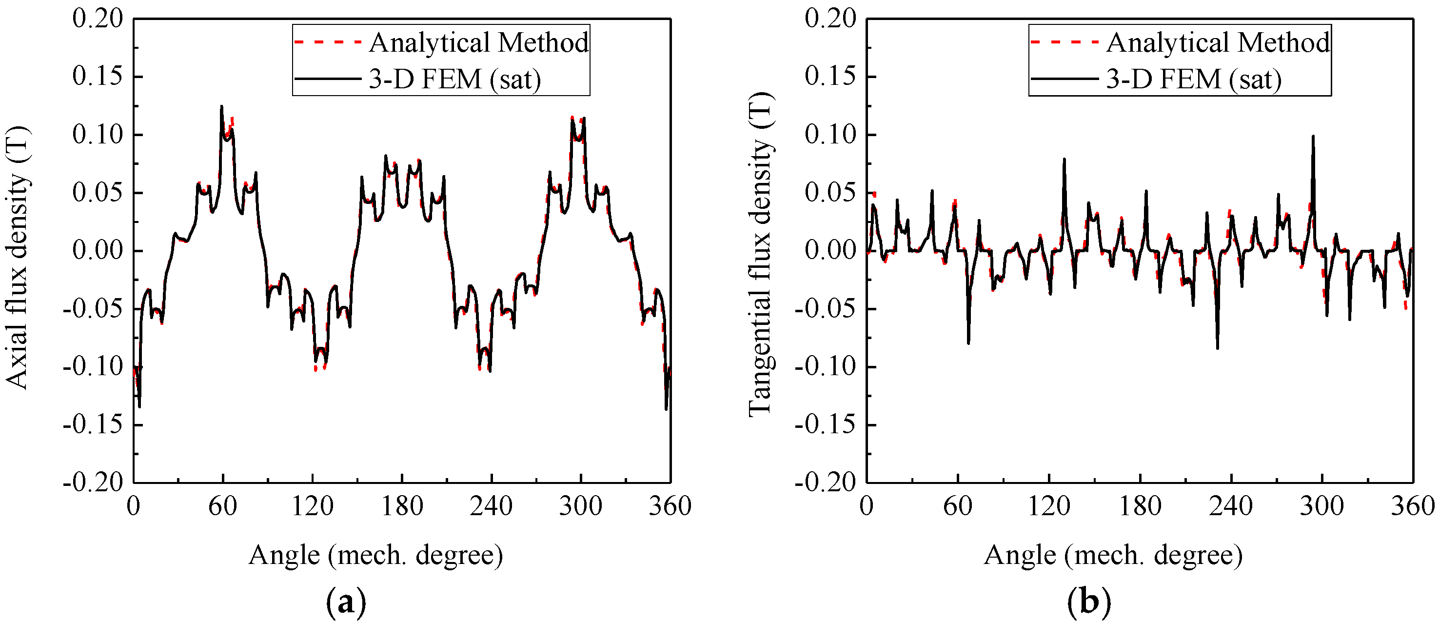
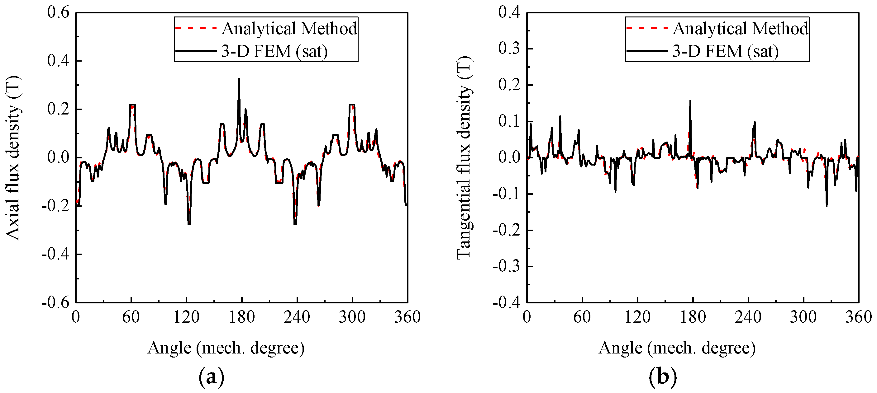
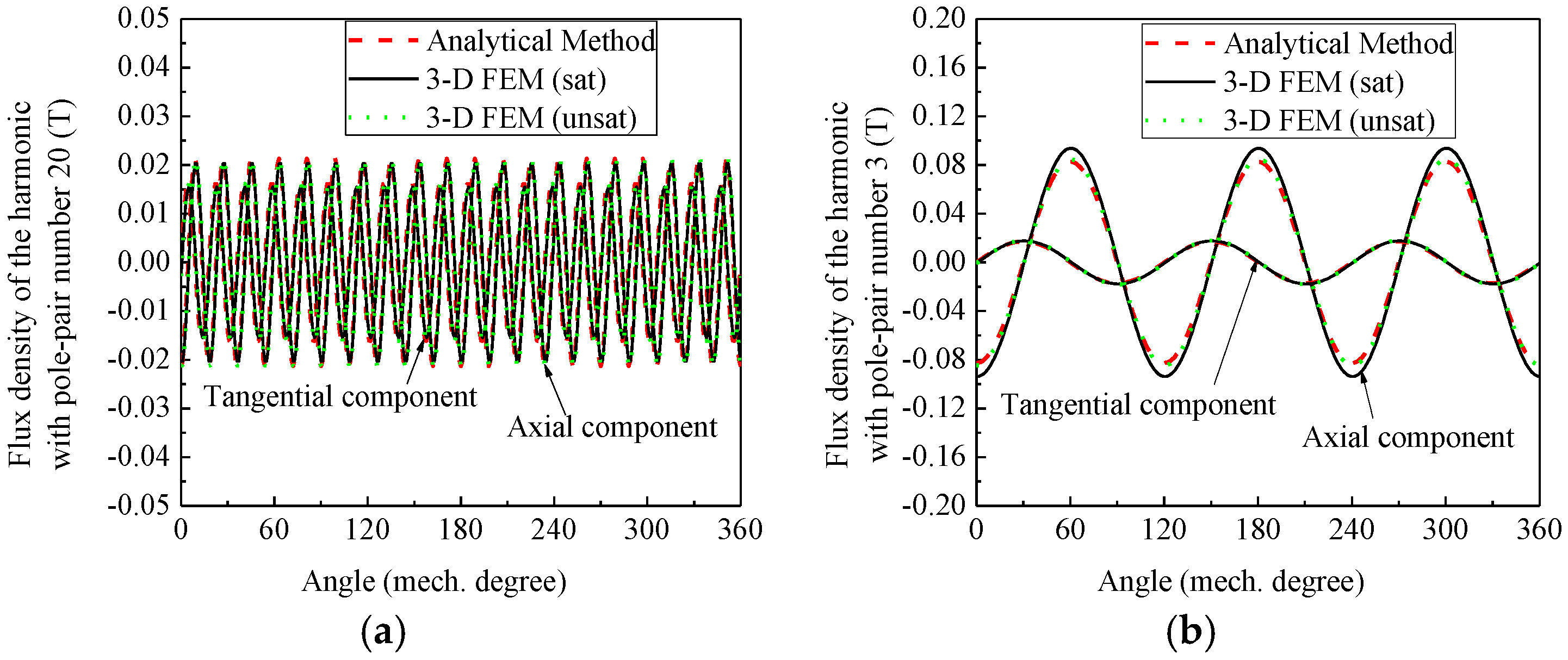
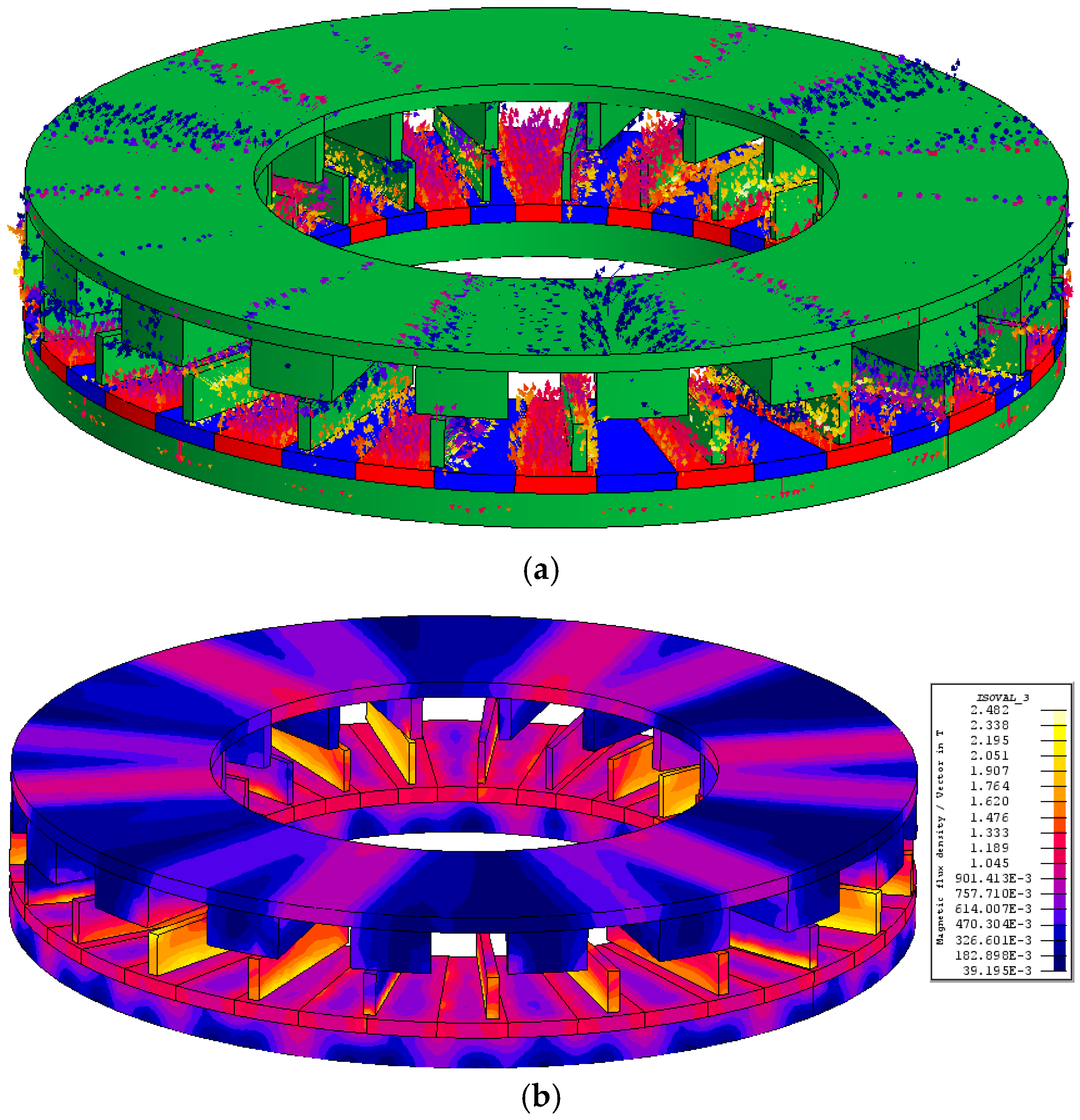
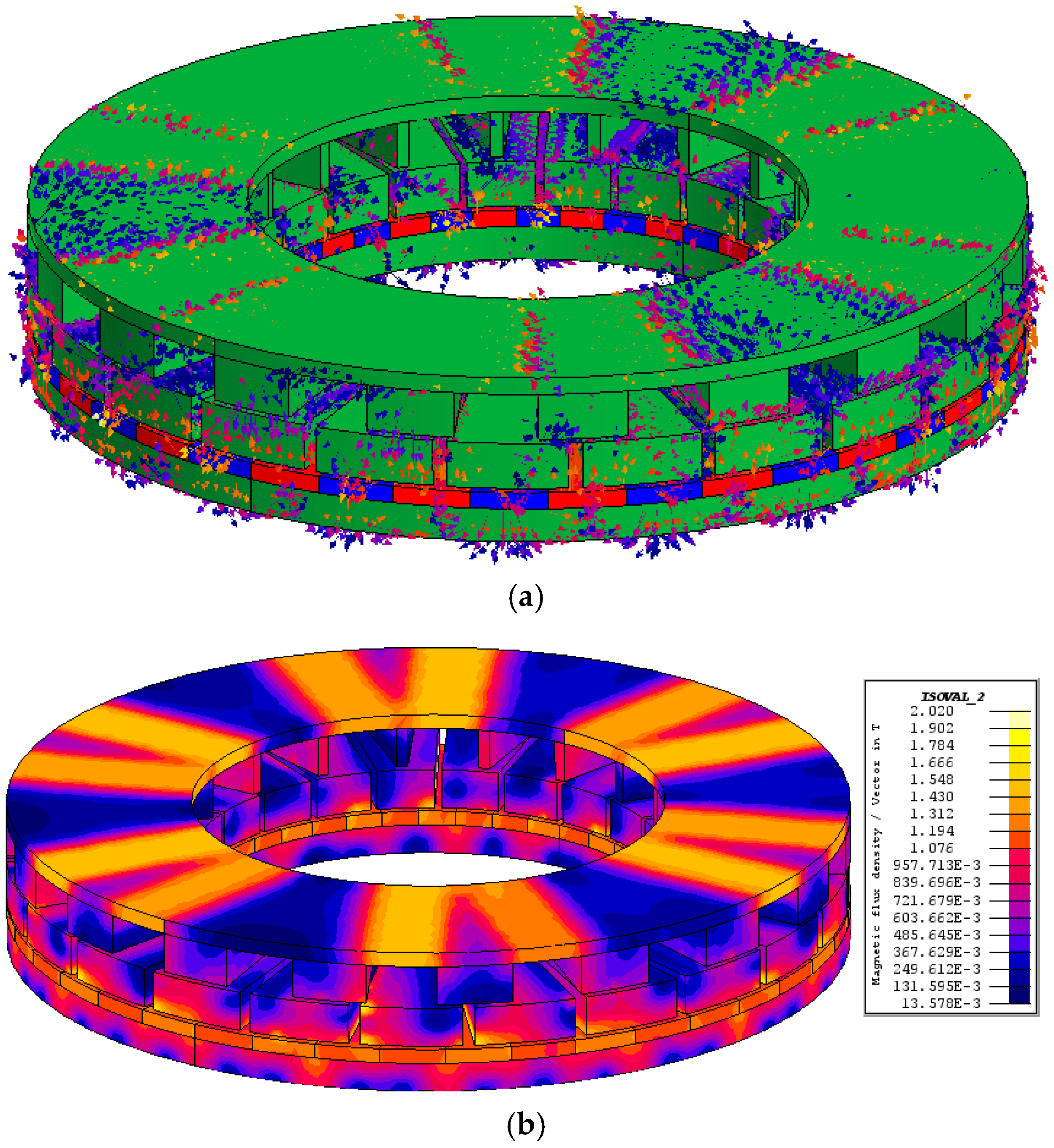
4.1. Magnetic-Field Distribution

Figure 7, Figure 8, Figure 9 and Figure 10 show the axial and tangential component of flux density at the middle of two air gaps produced by PMs and three-phase stator winding, respectively. The 3-D FEM (sat) simulation takes account of the saturation effect of FB, stator and PM rotor yoke. As can be observed, the predicted field distributions are well consistent with 3-D FEM results. It can also be seen that the modulation effect is significant with the existence of the modulating ring rotor.

Figure 11 shows the flux density distributions in the soft iron parts (stator, FB and PM rotor yoke) produced by PMs and three-phase stator winding, respectively. The results are obtained by 3-D FEM (sat). As the shape of stator tooth and FB is sector, flux density distribution in the stator teeth and FBs at the inner radius is more easily saturated than that at the outer radius.

It can be observed from Figure 11a that flux density in the FB adjacent to the inner air gap is deeply saturated, owning to the existence of pole-to-pole flux leakage. As magnetic field produced by three-phase stator winding is weaker than that by PMs, flux density in the FB produced by three-phase stator winding is much smaller than that produced by PMs. Saturation effect of the stator mainly depends on the amplitude of stator current.

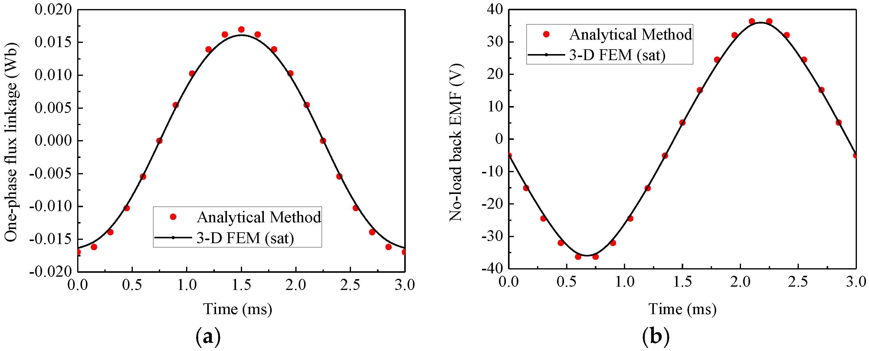
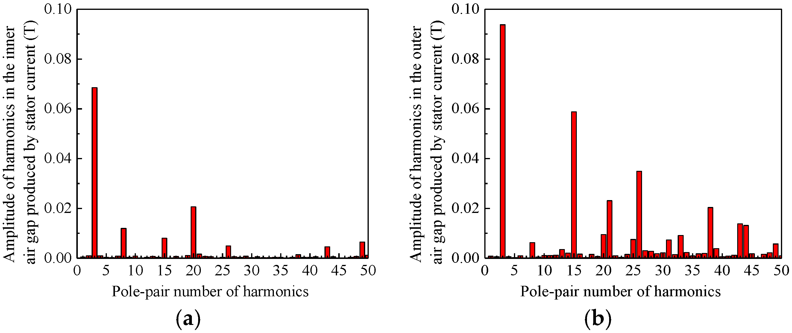
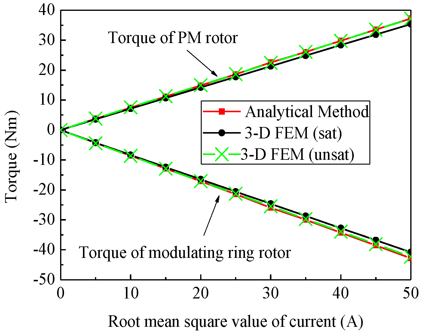
4.2. Electromagnetic Performance Prediction

One-phase flux linkage and no-load back EMF waveforms are shown in Figure 12. It can be seen that the proposed analytical model can predict no-load back EMF with a good precision, which demonstrates the validity of Equation (36). Compared with 3-D FEM (sat), amplitude of analytical result is 2.65% higher.

Figure 13 shows the cogging torque waveform on the PM rotor with the rotational speed of PM rotor 1000 rpm. It can be seen that when the PM rotor rotates by two full pole pitches, the fluctuation frequency of the cogging torque obtained by the analytical method is the same as with 3-D FEM (sat). The analytical and numerical results are in good accordance except for some points. The discrepancy between analytical predictions and simulations on the peak value of cogging toque is no more than 13%.

When PM rotor rotates from 0° to 18° (two full pole pitches) with the fixed stator current (I_a = I_b = −I_c/2), the static torque and axial force on two rotors are shown in Figure 14. As can be observed, the same trend occurs with the analytical and the 3-D FEM (sat) results. The torque and axial force of the analytical method are slightly higher than that of the 3-D FEM (sat). The error between analytical predictions and simulations on toque is no more than 8% while that on axial force is less than 11%, which means that the discrepancy between two methods is acceptable. Therefore, Equations (37)–(40) are verified.

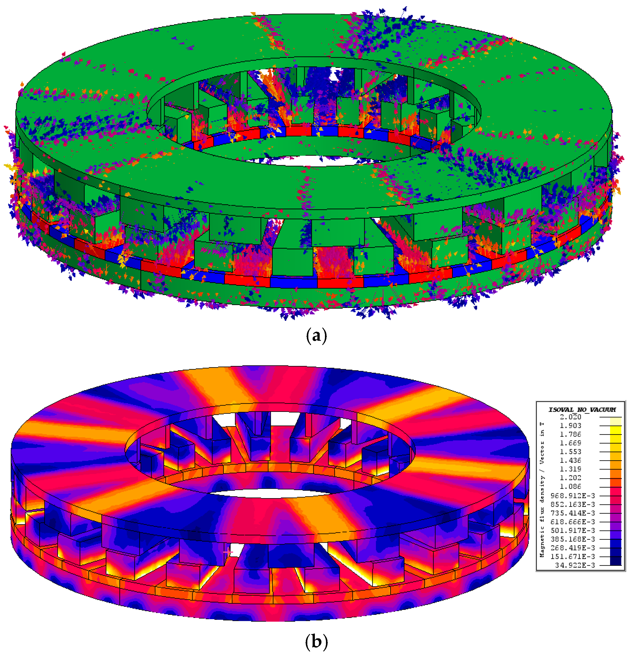
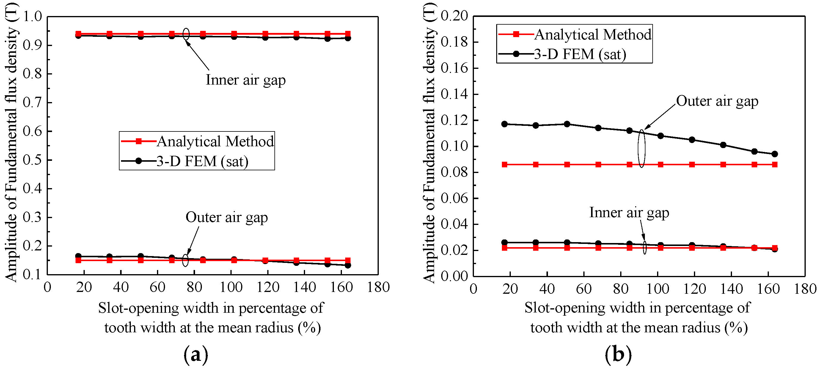
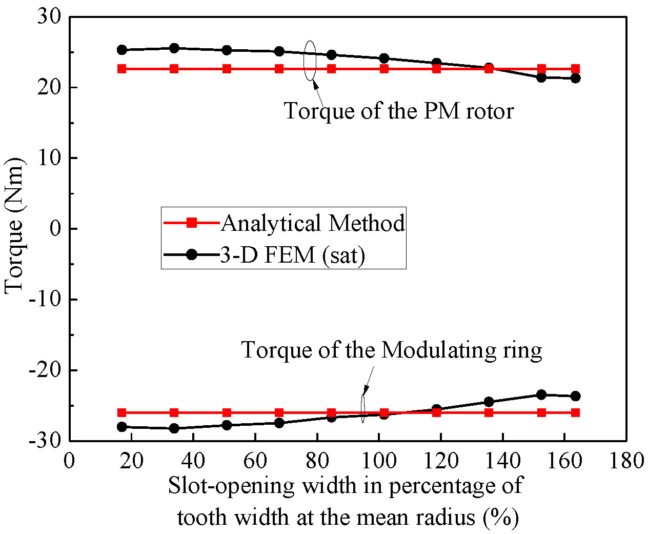
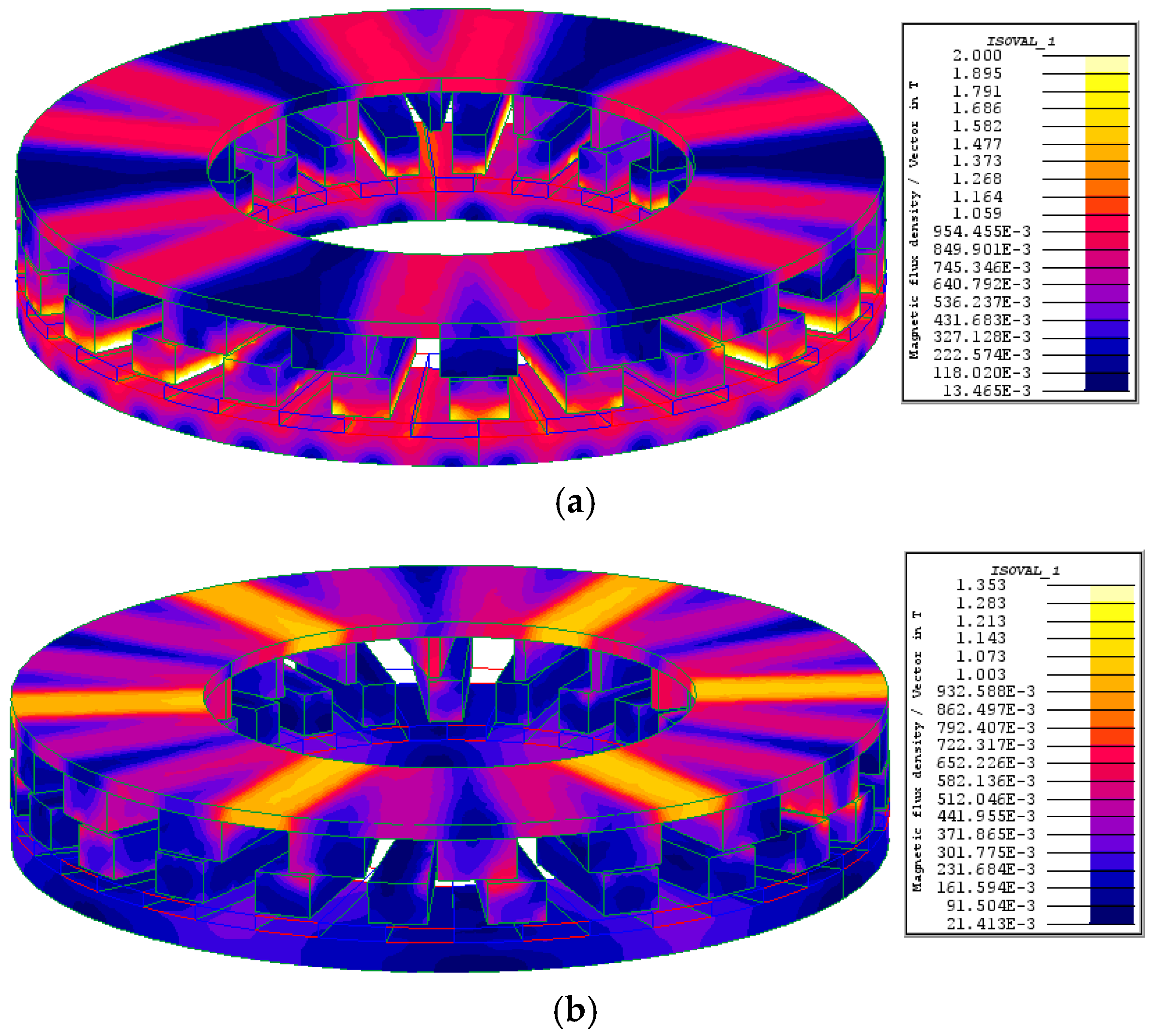
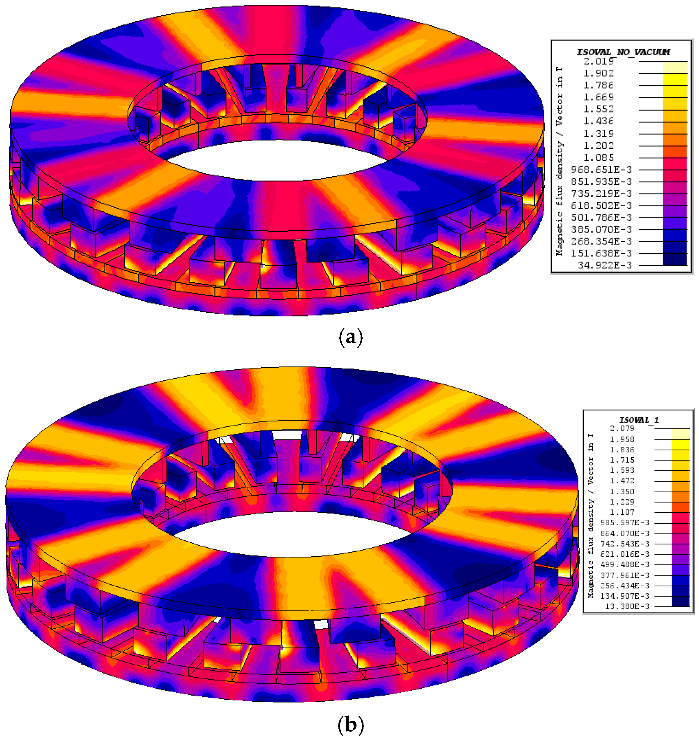
4.3. Saturation Effect

For the proposed analytical method, the saturation effect of the soft-magnetic material, which would introduce the calculation error in the magnetic field prediction, is not considered. Figure 15 shows the amplitude of harmonics in two air gaps produced by PMs, i.e., the corresponding space spectra of the axial component obtained by 3-D FEM (sat) in Figure 7a and Figure 8a. It can be seen that harmonic with the pole-pair number of 3 is the major modulated harmonic in the outer air gap, which is the same with P_s. Figure 16 is the amplitude of harmonics in two air gaps produced by three-phase stator winding, i.e., the corresponding space spectra of the axial component obtained by 3-D FEM (sat) in Figure 9a and Figure 10a. It can be seen that harmonic with the pole-pair number of 20 is the major modulated harmonic in the inner air gap, which is the same with P_p. Therefore, the pole-pair number of fundamental flux density in the inner air gap is 20 while that in the outer air gap is 3.

Figure 17 and Figure 18 show the fundamental flux density at the middle of two air gaps produced by PMs and three-phase stator winding, respectively. For the 3-D FEM (unsat) case, saturation effect of FB, stator and PM rotor yoke is neglected while for the 3-D FEM (sat) case, the corresponding saturation effect is determined by the B-H characteristic of the silicon steel sheet (DW 310-35). As can be observed in Figure 17 and Figure 18, the analytical results approximately consist with 3-D FEM (unsat) results whereas the difference exists between analytical results and 3-D FEM (sat) results, especially for the fundamental flux density in the outer air gap.

Figure 19 shows the flux density distributions in the soft iron parts (stator, FB and PM rotor yoke) under load condition with different excitation currents. The results are obtained by 3-D FEM (sat). It can be observed that flux density in the FB adjacent to the inner air gap is deeply saturated. The stator teeth are partially saturated at the inner radius. Moreover, saturation effect of the stator mainly depends on the stator current. The larger the excitation current is, the more significant the stator saturation will be.

Figure 20 shows the torque characteristics with different excitation currents (I_d = 0). It can be observed that the analytical results are in good accordance with 3-D FEM (unsat) results. The torque ration of the modulating ring with respect to the PM rotor is very close to −23/20, which agrees well with Equation (3). On the other hand, the magnetic saturation has an influence on the accuracy of the analytical method. With the increment of the excitation current, the effect of saturation is enhanced, resulting in higher discrepancy between analytical prediction and 3-D FEM (sat) simulation. The error between analytical method and 3-D FEM (sat) is less than 5.06%.

Figure 21 shows the torque characteristics with different air-gap thicknesses. As can be observed, analytical predictions follow the same trend with 3-D FEM (sat) simulations and the error between two methods on torque is more evident for the modulating ring rotor (within 8.73%) than the PM rotor (less than 4%). Figure 22 shows the flux density distributions in the soft iron parts under load condition with the air-gap thickness 1 mm and 0.5 mm, respectively. It can be seen that saturation in the FB and stator is more significant for the lower air gaps, resulting in larger difference between analytical and FEM results on torque of modulating ring rotor. Though scheme with higher power/torque density leads to higher discrepancy, the proposed analytical method is still valid for performance prediction with high precision.

4.4. End Effect

With the existence of FB, there is lots of radial flux leakage at the end spaces. Figure 23 shows the amplitude of fundamental flux density at the middle of two air gaps along the radial direction by 3-D FEM (sat). One can observe that the magnetic-field distribution is related to the radius. The amplitude of fundamental flux density is approximately constant in the middle part of the radius while it drops severely around the inner and outer radius. In addition, it can also be seen that the analytical results are close to the simulation results at the mean radius. The end effect is neglected for the analytical method by adopting the 2-D equivalent model at the mean radius instead of the 3-D model, which is one of the main reasons for the discrepancy between two methods for predicting electromagnetic performance.

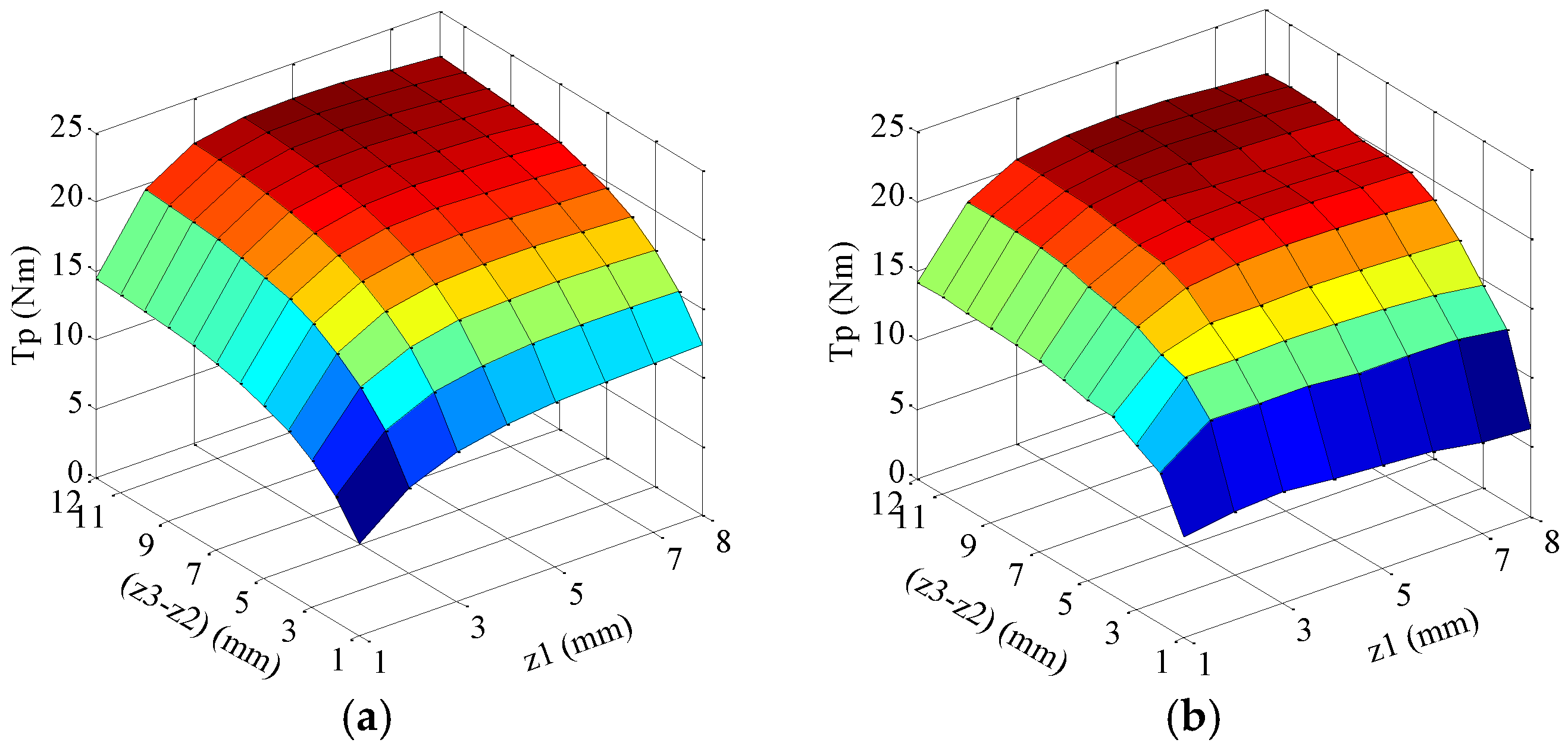
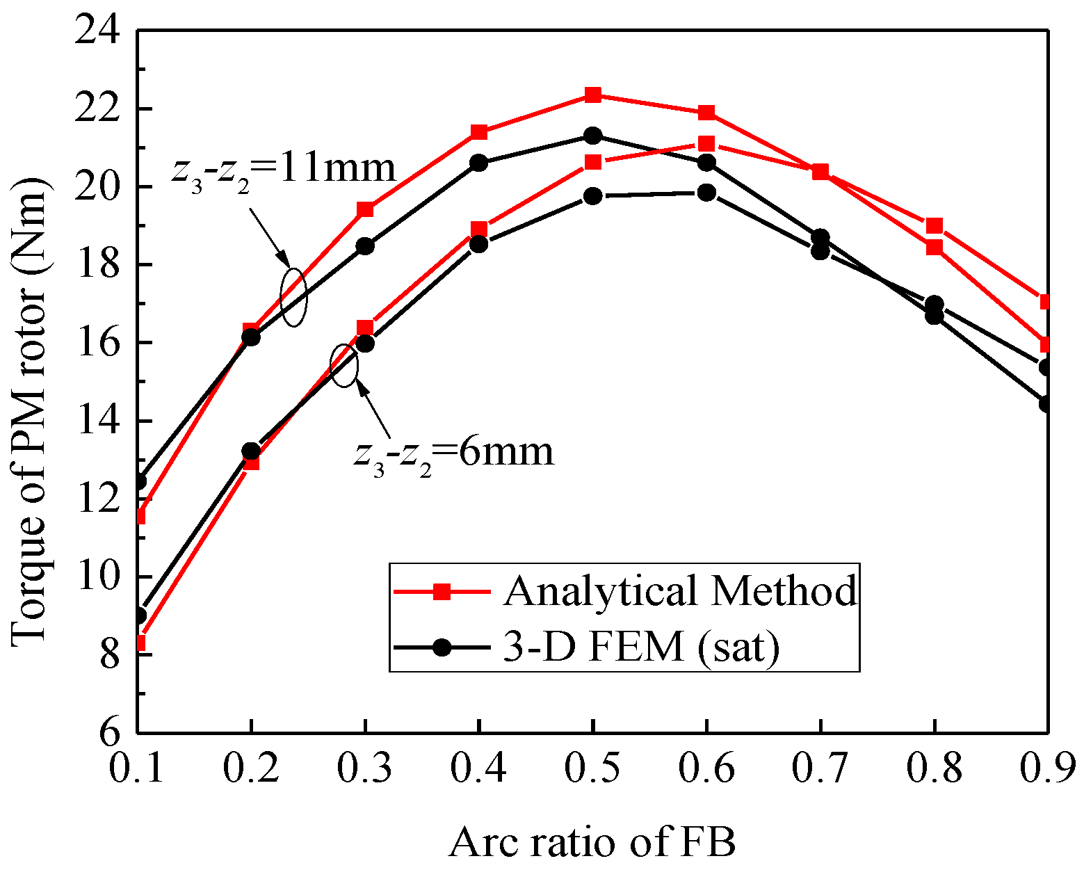
4.5. Influence of Key Parameters on the Performance

For the MFM-BDRM, arc ratio of FB is a critical parameter that determines the modulation effect. Figure 24, Figure 25 and Figure 26 show the flux density distribution with arc ratio of FB 0.1, 0.5 and 0.9, respectively. As can be seen, the arc ratio of FB has an essential impact on the saturation in the FB and pole-to-pole flux leakage. Deep saturation accrues in the FB with arc ratio of FB 0.1 and the saturation effect in FB decreases with the increment of arc ratio of FB. Moreover, pole-to-pole flux leakage is obvious with large arc ratio of FB, especially when arc ratio of FB is 0.9.

Figure 27 shows the effect of arc ratio of FB on the PM torque value for two schemes with different thickness of FB. The error between analytical method and 3-D FEM (sat) is less than 10.6%. However, it is important to note that the analytical and the finite element analysis (FEA) computations follow the same trend for each scheme and they both achieve the optimum value with arc ratio of FB 0.6 and 0.5 for the scheme with the thickness of FB 6 mm and 11 mm, respectively.

The influence of the magnet thickness combined with the FB thickness on the performance of the axial MFM-BDRM is shown in Figure 28. It can be seen that the magnet thickness and the FB thickness have a prominent effect on the torque transmission capability, with the difference between the maximum and the minimum value more than 15 Nm. What is more, the analytical method and 3-D FEM (sat) share the same changing trend. For a certain FB thickness, the torque increases with the magnet thickness increasing, and arrives at the maximum value with the magnet thickness 4 mm, and then drop. For a certain magnet thickness, with the increment of the FB thickness, the torque increases at first and then remains approximately constant. When the FB thickness is thin from 1 mm to 3 mm, the difference between analytical method and 3-D FEM (sat) is relatively large, due to the severe saturation of the main flux path. For the FB thickness larger than 3 mm, the error between analytical predictions and simulations on toque is no more than 9.5%.

4.6. Application Scope

From the assessment above, it can be inferred that the 2-D analytical model in Figure 3 can accurately predict the performance of the axial MFM-BDRM with open slot. Whether the proposed model is suitable for the machine with semi-closed slot is discussed below. Figure 29 shows the variation of the amplitude of fundamental flux density at the middle of two air gaps with the slot-opening width in percentage of tooth width at the mean radius. It can be seen that the amplitude of fundamental flux density decreases with the increment of slot-opening width, especially in the outer air gap with the stator armature winding excitation. The analytical method could not capture the fluctuation in the flux density with the change of slot-opening width, and the difference between the analytical predictions and simulations is within 26%.

Figure 30 shows the torque characteristics with different slot-opening widths in percentage of tooth width at the mean radius. It can be seen that the absolute value of the torque decreases with the increment of slot-opening width, which agrees well with the variation of fundamental flux density in two air gaps. Though the analytical method could not reflect the trend of the torque with slot-opening width, the error of analytical result on torque is less than 11%. It means that the proposed analytical method can also be used for performance prediction of the semi-closed-slot machine with good precision.

To better situate when the proposed analytical method can be used or not, drawback of the proposed analytical method is discussed below. Figure 31 shows the cogging torque characteristics with different slot-opening widths in percentage of tooth width at the mean radius. It can be seen that the peak value of the cogging torque increases with the increment of slot-opening width. However, the analytical method could not reflect the trend of the cogging torque with slot-opening width. As can be observed, the proposed analytical method exhibits the limitation on cogging torque prediction for the semi-closed-slot machine with small slot-opening width.

As the soft-magnetic material is simplified to have infinite magnetic permeability, the proposed method cannot be used for the eddy current calculation. To obtain eddy loss in iron and PM parts, saturation effect in soft iron parts should be taken into account. The further investigation of the axial MFM-BDRM would focus on the loss prediction by using analytical method.

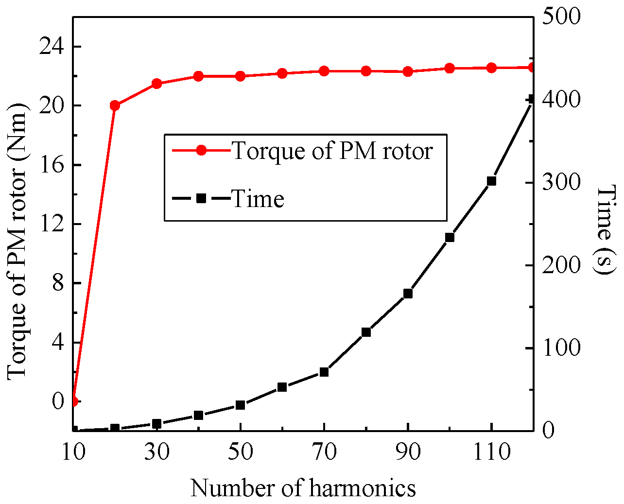
4.7. Computing Time Evaluation

To show the influence of the number of harmonics used in the analytical computation, Figure 32 respectively gives the PM torque and computing time vs. the number of harmonics. It can be inferred that 30 harmonic terms are sufficient to predict the torque with a good precision. Moreover, with the increment of the number of harmonics, the calculation time increases exponentially. The analytical computation takes about 8.8 s with the choice of 30 harmonic terms whereas the 3-D FEM simulation lasts 30 min with 275,307 mesh nodes. As the analytical computation is much faster with the error no more than 11%, it can be used as an effective tool in the preliminary design process of the axial MFM-BDRM.

5. Conclusions

A 2-D analytical method has been proposed for predicting the magnetic-field distribution in a novel axial-flux magnetic-geared machine.

(1)

The analytical expressions for open-circuit and armature reaction field distribution by considering the stator slotting and modulation effect have been derived from a set of Laplace’s or Poisson’s equations with corresponding boundary conditions. The magnetic-field predictions show good consistency with 3-D FEM results.

(2)

The no-load back EMF, torque and axial force have been obtained by adopting the predicted flux density at the mean radius instead of the actual 3-D distribution of the magnetic field. The 2-D analytical method overestimates the machine performance by less than 11%. The discrepancy is mainly due to the fact that the analytical method assumes unsaturation of the soft-magnetic material and no end effect.

(3)

As the analytical and 3-D FEM computation follow the same trend in evaluating the torque with less calculation time and more flexibility, it can be used as an effective tool for the initial design procedure of the axial MFM-BDRM with open slot.

(4)

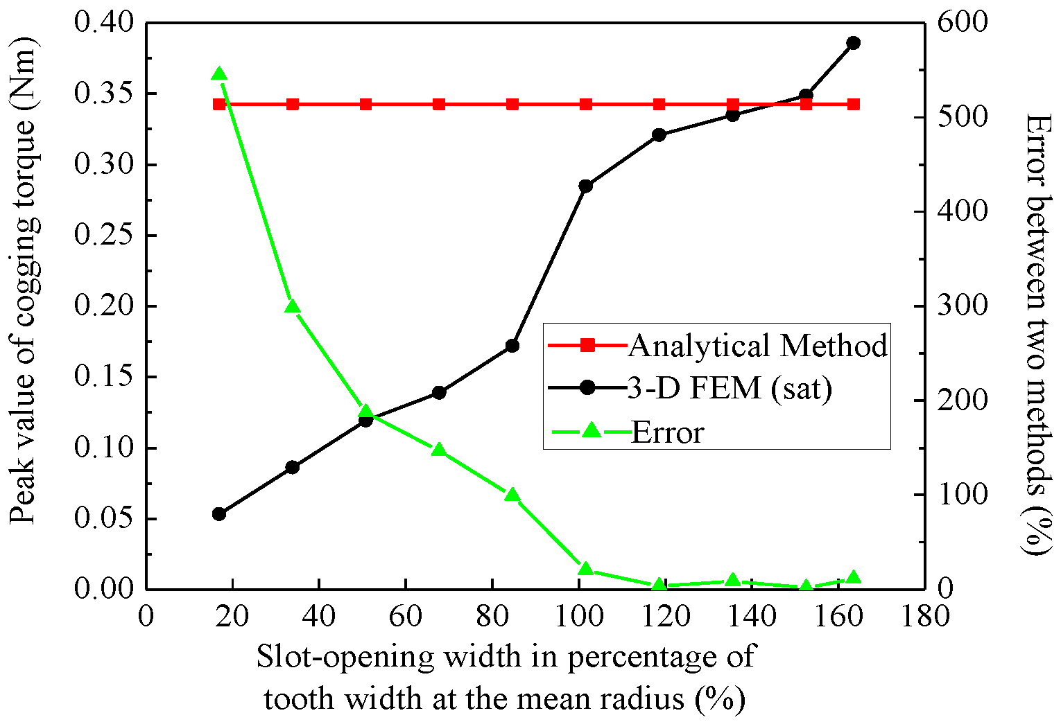
Though the proposed method could not capture the fluctuation in torque with the change of slot-opening width, it can be used for performance prediction of the open-slot or the semi-closed-slot machine with high precision.

References

1. Nordlund, E.; Eriksson, S. Test and verification of a four-quadrant transducer for HEV applications. In Proceedings of the IEEE Vehicle Power and Propulsion Conference, Chicago, IL, USA, 7–9 September 2005.
2. Hoeijmakers, M.J.; Ferreira, J.A. The electric variable transmission. IEEE Trans. Ind. Appl. 2006, 42, 1092–1100. [Google Scholar] [CrossRef]
3. Xu, L.; Zhang, Y.; Wen, X. Multioperational modes and control strategies of dual-mechanical-port machine for hybrid electrical vehicles. IEEE Trans. Ind. Appl. 2009, 45, 747–755. [Google Scholar] [CrossRef]
4. Shumei, C.; Yongjie, Y.; Tiecheng, W. Research on switched reluctance double-rotor motor used for hybrid electric vehicle. In Proccedings of the International Conference on Electrical Machines and Systems, Wuhan, China, 17–20 October 2008; pp. 3393–3396.
5. Zheng, P.; Liu, R.; Thelin, P.; Nordlund, E.; Sadarangani, C. Research on the cooling system of a 4QT prototype machine used for HEV. IEEE Trans. Energy Convers. 2008, 23, 61–67. [Google Scholar] [CrossRef]
6. Sun, X.; Cheng, M. Thermal analysis and cooling system design of dual mechanical port machine for wind power application. IEEE Trans. Ind. Electron. 2013, 60, 1724–1733. [Google Scholar] [CrossRef]
7. Bai, J.; Liu, Y.; Sui, Y.; Tong, C.; Zhao, Q.; Zhang, J. Investigation of the cooling and thermal-measuring system of a compound-structure permanent-magnet synchronous machine. Energies 2014, 7, 1393–1426. [Google Scholar] [CrossRef]
8. Cavagnino, A.; Lazzari, M.; Profumo, F.; Tenconi, A. A comparison between the axial flux and the radial flux structures for PM synchronous motors. IEEE Trans. Ind. Appl. 2002, 38, 1517–1524. [Google Scholar] [CrossRef]
9. Huang, S.; Aydin, M.; Lipo, T.A. A direct approach to electrical machine performance evaluation: Torque density assessment and sizing optimization. In Proceedings of the 2002 Xth International Conference on Electrical Machines (ICEM), Bruges, Belgium, 26–28 August 2002.
10. Mezani, S.; Atallah, K.; Howe, D. A high-performance axial-field magnetic gear. J. Appl. Phys. 2006, 99. [Google Scholar] [CrossRef]
11. Niguchi, N.; Hirata, K.; Zaini, A.; Nagai, S. Proposal of an axial-type magnetic-geared motor. In Proceedings of the 2012 XXth International Conference on Electrical Machines (ICEM), Marseille, France, 2–5 September 2012; pp. 738–743.
12. Ho, S.L.; Niu, S.; Fu, W.N. Design and analysis of a novel axial-flux electric machine. IEEE Trans. Magn. 2011, 47, 4368–4371. [Google Scholar] [CrossRef]
13. Johnson, M.; Gardner, M.C.; Toliyat, H.A. Design and analysis of an axial flux magnetically geared generator. In Proceedings of the 2015 IEEE Energy Conversion Congress and Exposition (ECCE), Montreal, QC, Canada, 20–24 September 2015; pp. 6511–6518.
14. Wang, R.J.; Brönn, L.; Gerber, S.; Tlali, P.M. Design and evaluation of a disc-type magnetically geared PM wind generator. In Proceedings of the 2013 Fourth International Conference on Power Engineering, Energy and Electrical Drives (POWERENG), Istanbul, Turkey, 13–17 May 2013; pp. 1259–1264.
15. Rojas, A.; Tapia, J.A.; Valenzuela, M.A. Axial flux PM machine design with optimum magnet shape for constant power region capability. In Proceedings of the 18th International Conference on Electrical Machines, ICEM 2008, Vilamoura, Portugal, 6–9 September 2008; pp. 1–6.
16. Zheng, P.; Song, Z.; Bai, J.; Tong, C.; Yu, B. Research on an axial magnetic-field-modulated brushless double rotor machine. Energies 2013, 6, 4799–4829. [Google Scholar] [CrossRef]
17. Dubas, F.; Espanet, C. Analytical solution of the magnetic field in permanent-magnet motors taking into account slotting effect: No-load vector potential and flux density calculation. IEEE Trans. Magn. 2009, 45, 2097–2109. [Google Scholar] [CrossRef]
18. Lubin, T.; Mezani, S.; Rezzoug, A. 2-D exact analytical model for surface-mounted permanent-magnet motors with semi-closed slots. IEEE Trans. Magn. 2011, 47, 479–492. [Google Scholar] [CrossRef]
19. Rahideh, A.; Korakianitis, T. Analytical magnetic field calculation of slotted brushless permanent-magnet machines with surface inset magnets. IEEE Trans. Magn. 2012, 48, 2633–2649. [Google Scholar] [CrossRef]
20. Zhu, Z.Q.; Howe, D. Instantaneous magnetic field distribution in brushless permanent magnet DC motors, Part III: Effect of stator slotting. IEEE Trans. Magn. 1993, 29, 143–151. [Google Scholar] [CrossRef]
21. Lubin, T.; Mezani, S.; Rezzoug, A. Analytical computation of the magnetic field distribution in a magnetic gear. IEEE Trans. Magn. 2010, 46, 2611–2621. [Google Scholar] [CrossRef]
22. Jian, L.; Xu, G.; Mi, C.C.; Chau, K.T.; Chan, C.C. Analytical method for magnetic field calculation in a low-speed permanent-magnet harmonic machine. IEEE Trans. Energy Convers. 2011, 26, 862–870. [Google Scholar] [CrossRef] [Green Version]
23. Zhang, Y.J.; Jing, L.B. Exact analytical method for magnetic field computation in the concentric magnetic gear with Halbach permanent-magnet arrays. In Proceedings of the 2013 IEEE International Conference on Applied Superconductivity and Electromagnetic Devices, Beijing, China, 25–27 October 2013.
24. Lubin, T.; Mezani, S.; Rezzoug, A. Development of a 2-D analytical model for the electromagnetic computation of axial-field magnetic gears. IEEE Trans. Magn. 2013, 49, 5507–5521. [Google Scholar] [CrossRef]
Figure 1. Three-dimensional (3-D) configuration of the investigated machine: (a) overall view; and (b) exploded view.
Energies 09 00589 g001
Figure 2. The axial magnetic-field-modulated brushless double-rotor machine (MFM-BDRM) system. PM: permanent magnet.
Energies 09 00589 g002
Figure 3. Two-dimensional (2-D) analytical model of the axial-flux magnetic-geared machine.
Energies 09 00589 g003
Figure 4. Axial magnetization distribution along the θ direction.
Energies 09 00589 g004
Figure 5. Distributed current sheet of three-phase stator winding.
Energies 09 00589 g005
Figure 6. Layout of one-phase winding of the axial MFM-BDRM.
Energies 09 00589 g006
Figure 7. Flux density distribution in the inner air-gap region produced by PMs: (a) axial component; and (b) tangential component.
Energies 09 00589 g007
Figure 8. Flux density distribution in the outer air-gap region produced by PMs: (a) axial component; and (b) tangential component.
Energies 09 00589 g008
Figure 9. Flux density distribution in the inner air-gap region produced by three-phase stator winding: (a) axial component; and (b) tangential component.
Energies 09 00589 g009
Figure 10. Flux density distribution in the outer air-gap region produced by three-phase stator winding: (a) axial component; and (b) tangential component.
Energies 09 00589 g010
Figure 11. Flux density distributions in the soft iron parts: (a) produced by PMs; and (b) produced by three-phase stator winding.
Energies 09 00589 g011
Figure 12. One-phase flux linkage and no-load back electromotive force (EMF) waveforms: (a) one-phase flux linkage waveform; and (b) no-load back EMF waveform.
Energies 09 00589 g012
Figure 13. Cogging torque waveform on the PM rotor with the rotational speed of PM rotor 1000 rpm.
Energies 09 00589 g013
Figure 14. The static torque and axial force characteristics with the PM rotor rotating by two full pole pitches: (a) torque; and (b) axial force.
Energies 09 00589 g014
Figure 15. Amplitude of harmonics in two air gaps produced by PMs: (a) in the inner air gap; and (b) in the outer air gap.
Energies 09 00589 g015
Figure 16. Amplitude of harmonics in two air gaps produced by three-phase stator winding: (a) in the inner air gap; and (b) in the outer air gap.
Energies 09 00589 g016
Figure 17. Fundamental flux density in two air-gap regions produced by PMs: (a) inner air gap; and (b) outer air gap.
Energies 09 00589 g017
Figure 18. Fundamental flux density in two air-gap regions produced by three-phase stator winding: (a) inner air gap; and (b) outer air gap.
Energies 09 00589 g018
Figure 19. Flux density distributions in the soft iron parts with different stator currents: (a) I = 30 A; and (b) I = 50 A.
Energies 09 00589 g019
Figure 20. Variations of torque with excitation current.
Energies 09 00589 g020
Figure 21. Variations of torque with different air-gap thicknesses.
Energies 09 00589 g021
Figure 22. Flux density distributions in the soft iron parts with different air-gap thicknesses: (a) 1 mm; and (b) 0.5 mm.
Energies 09 00589 g022
Figure 23. Variation of fundamental flux density at the middle of two air gaps with the radius: (a) under no-load condition; and (b) under load condition.
Energies 09 00589 g023
Figure 24. Flux density distribution with arc ratio of FB 0.1: (a) vector distribution; and (b) iso-value distribution.
Energies 09 00589 g024
Figure 25. Flux density distribution with arc ratio of FB 0.5: (a) vector distribution; and (b) Iso-value distribution.
Energies 09 00589 g025
Figure 26. Flux density distribution with arc ratio of FB 0.9: (a) vector distribution; (b) Iso-value distribution.
Energies 09 00589 g026
Figure 27. Influence of arc ratio of FB on the PM torque.
Energies 09 00589 g027
Figure 28. Influence of the magnet thickness combined with FB thickness on the PM torque: (a) analytical results; and (b) 3-D finite element method (FEM) (sat) simulation results.
Energies 09 00589 g028
Figure 29. Variation of fundamental flux density at the middle of two air gaps with the slot-opening width in percentage of tooth width at the mean radius: (a) PM rotor excitation; and (b) stator armature winding excitation.
Energies 09 00589 g029
Figure 30. Variations of torque with slot-opening width in percentage of tooth width at the mean radius.
Energies 09 00589 g030
Figure 31. Variations of cogging torque with slot-opening width in percentage of tooth width at the mean radius.
Energies 09 00589 g031
Figure 32. Influence of the number of harmonic terms.
Energies 09 00589 g032