
Numerical Investigation of Aerodynamic Performance and Loads of a Novel Dual Rotor Wind Turbine


Abstract
:1. Introduction
2. Numerical Method
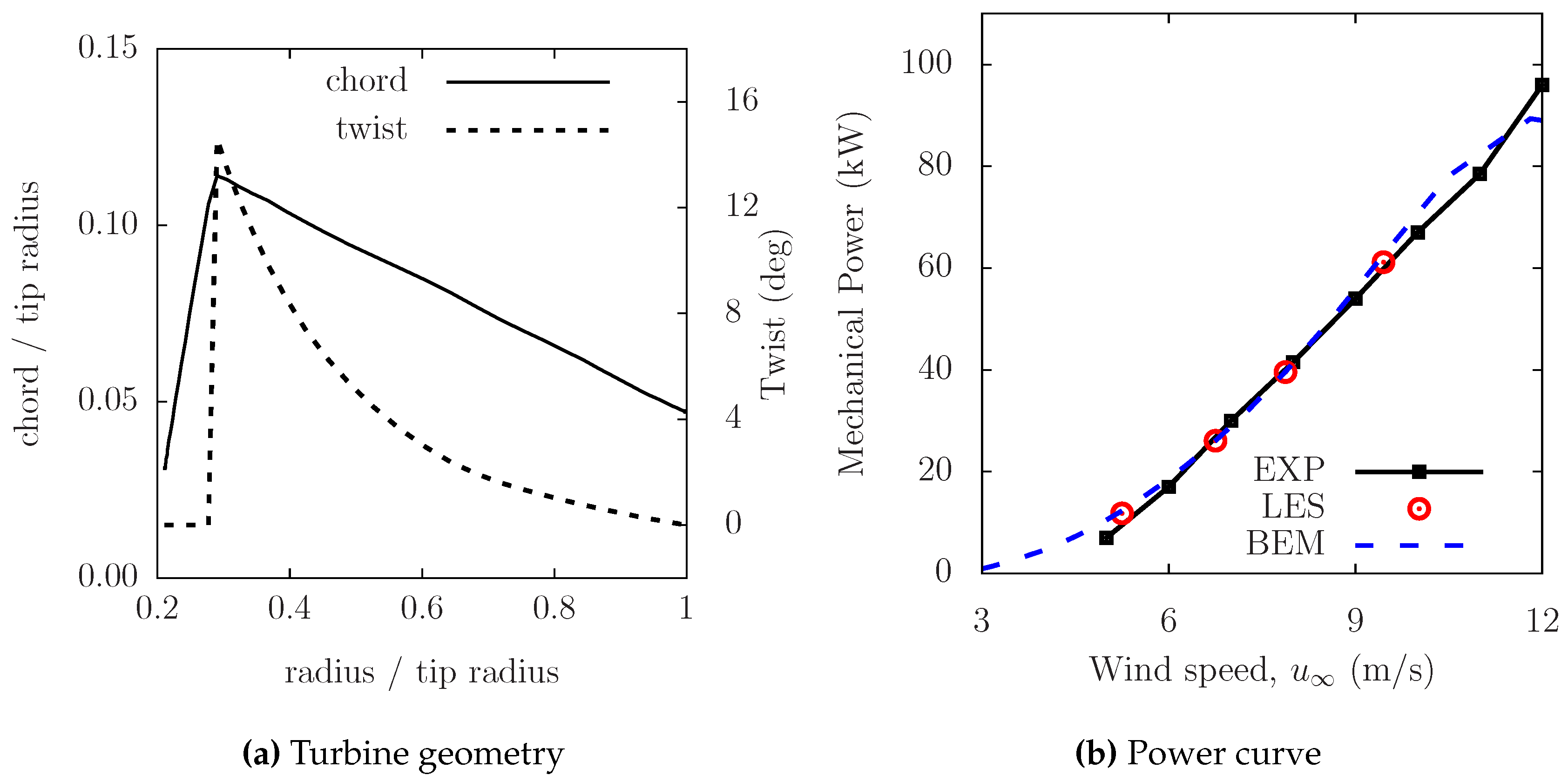
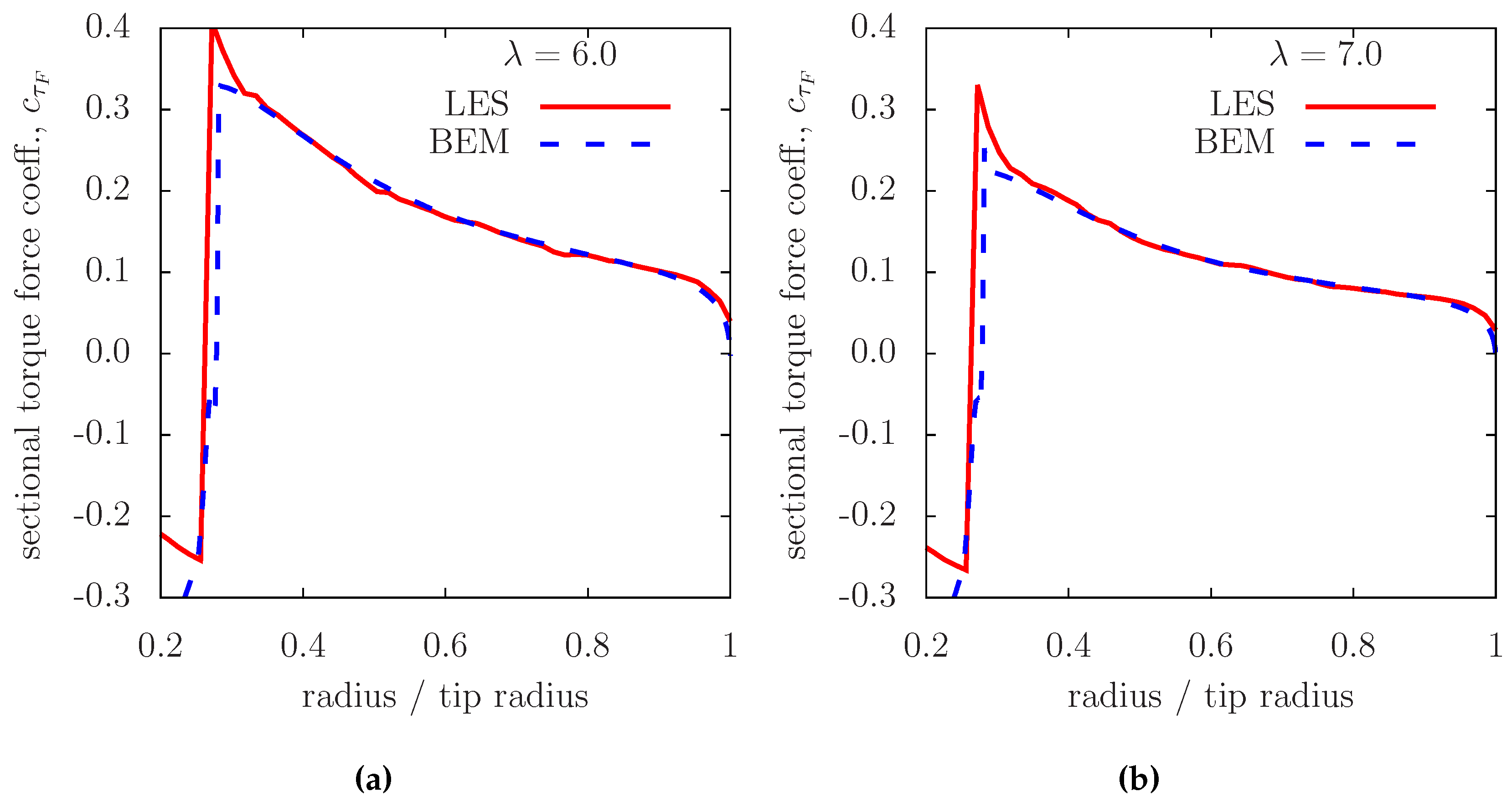
Validation
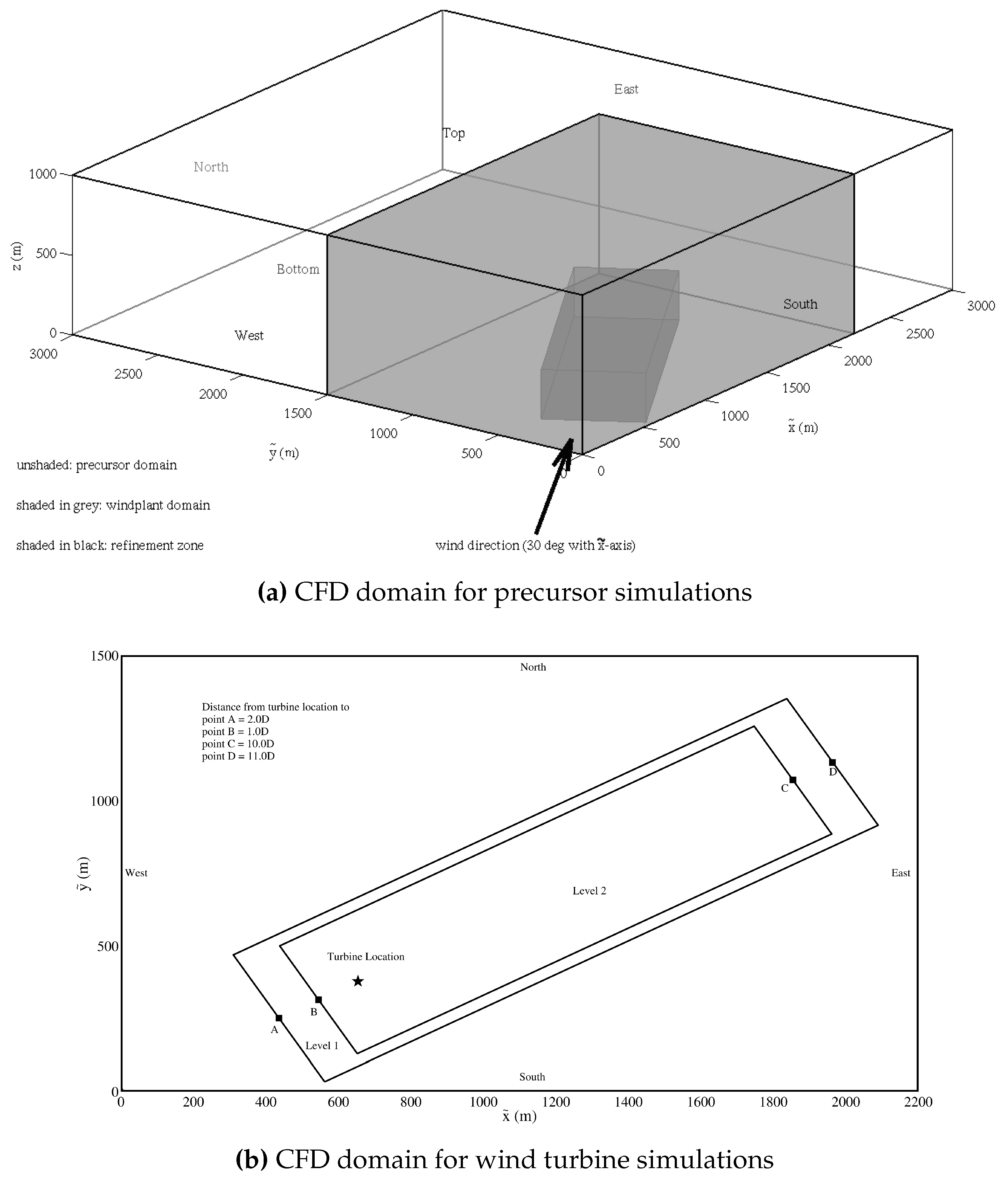
3. Computational Setup
4. Results and Discussion
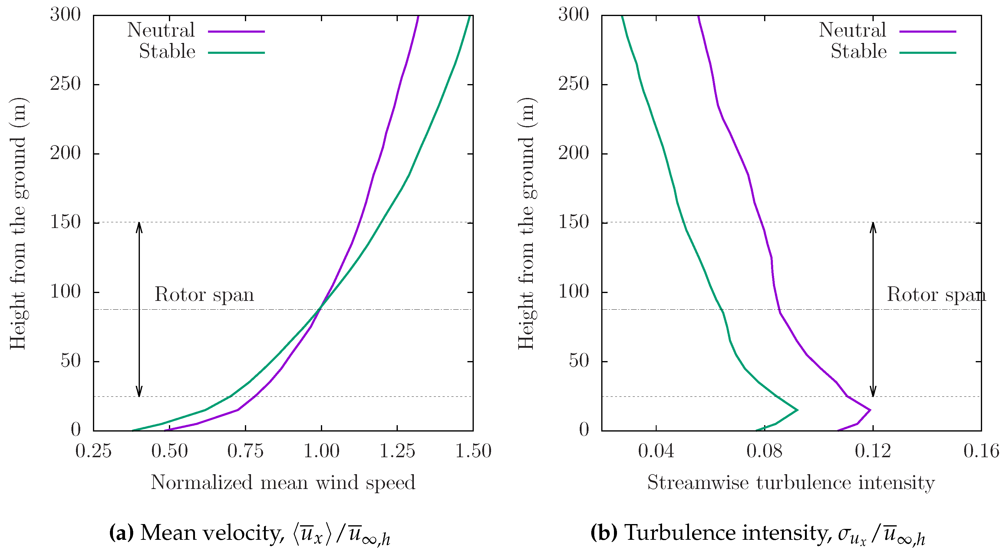
4.1. Atmospheric Boundary Layer
4.2. Aerodynamic Performance
4.2.1. Root Loss Mitigation
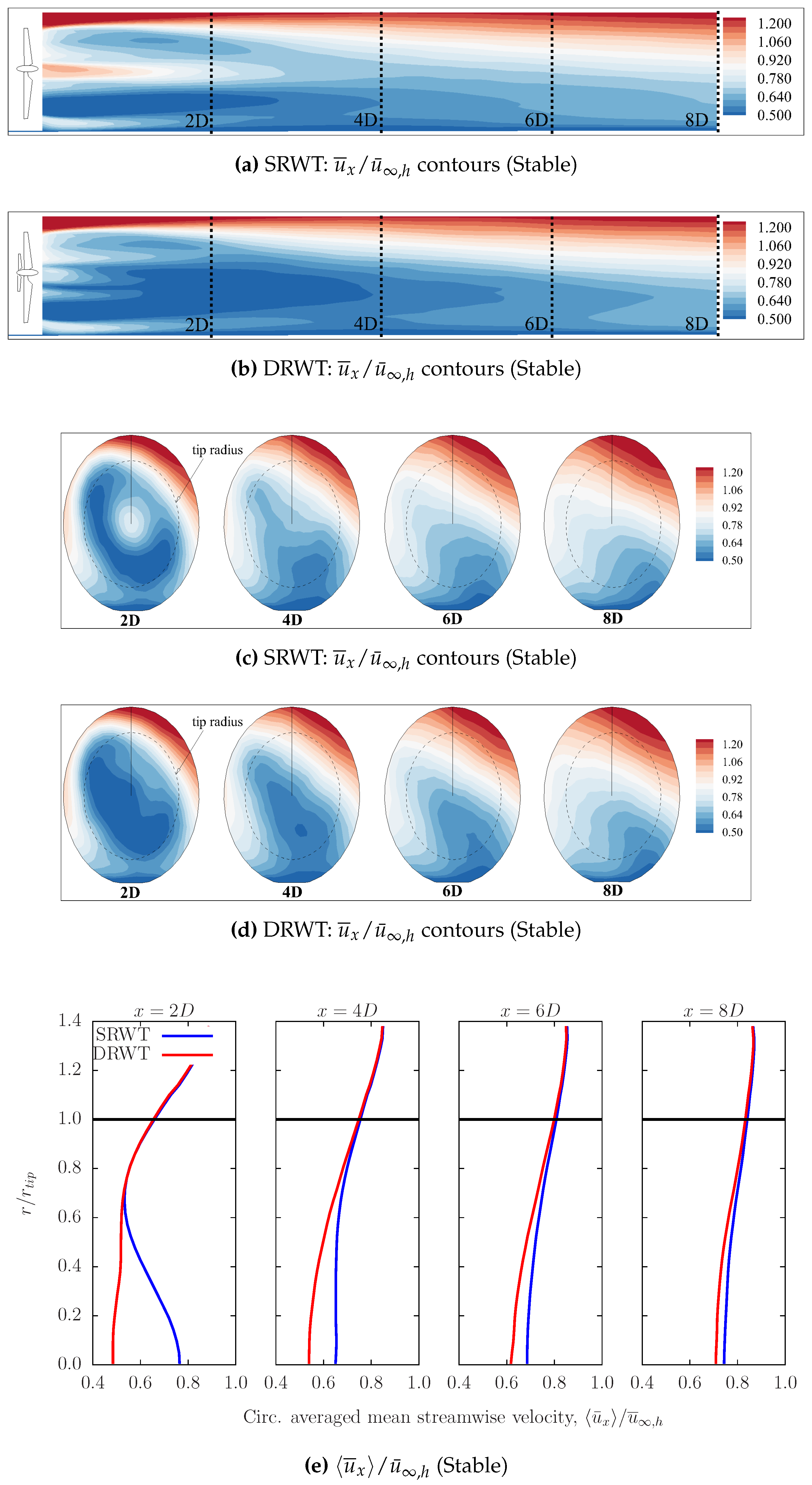
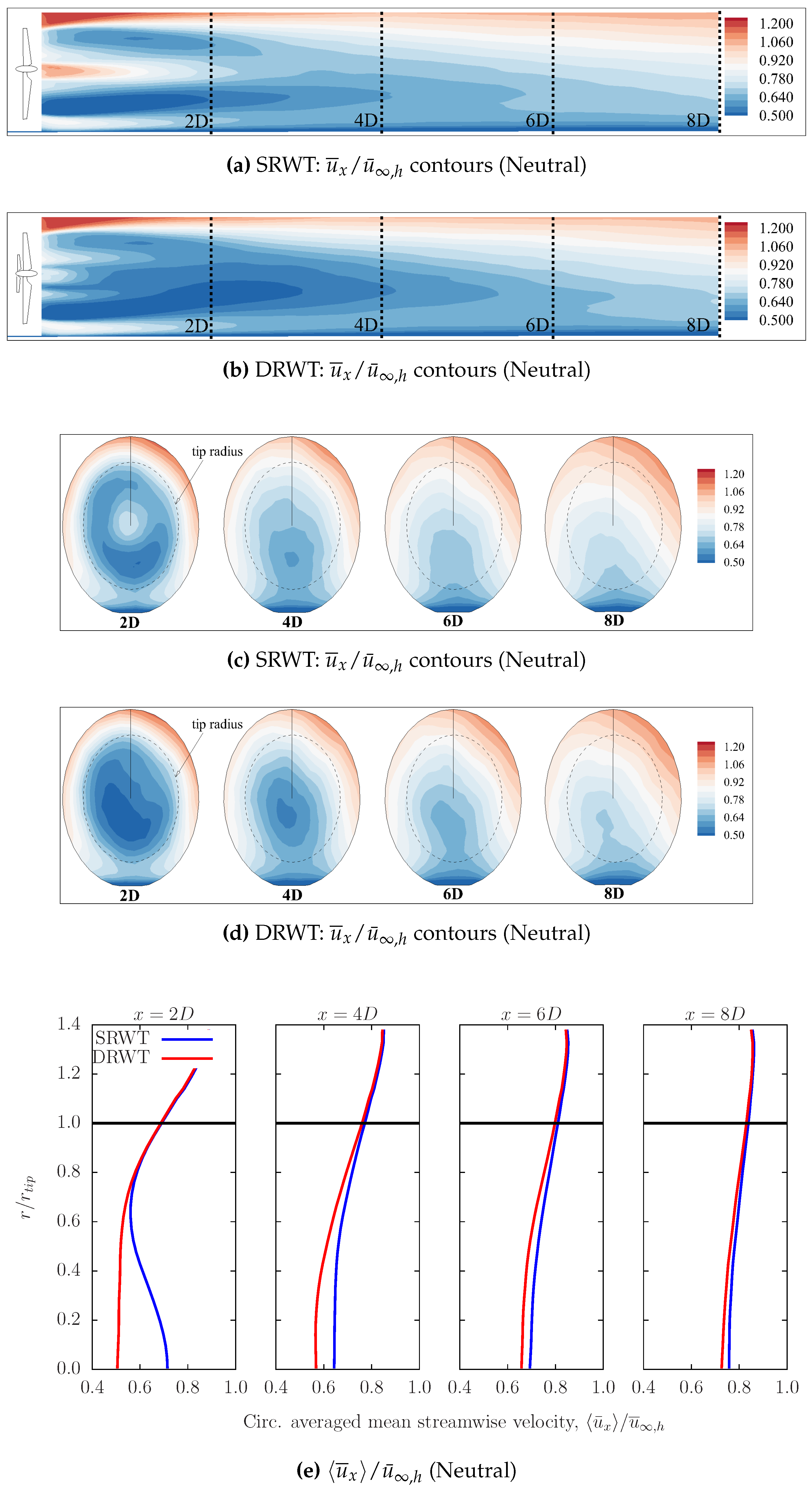
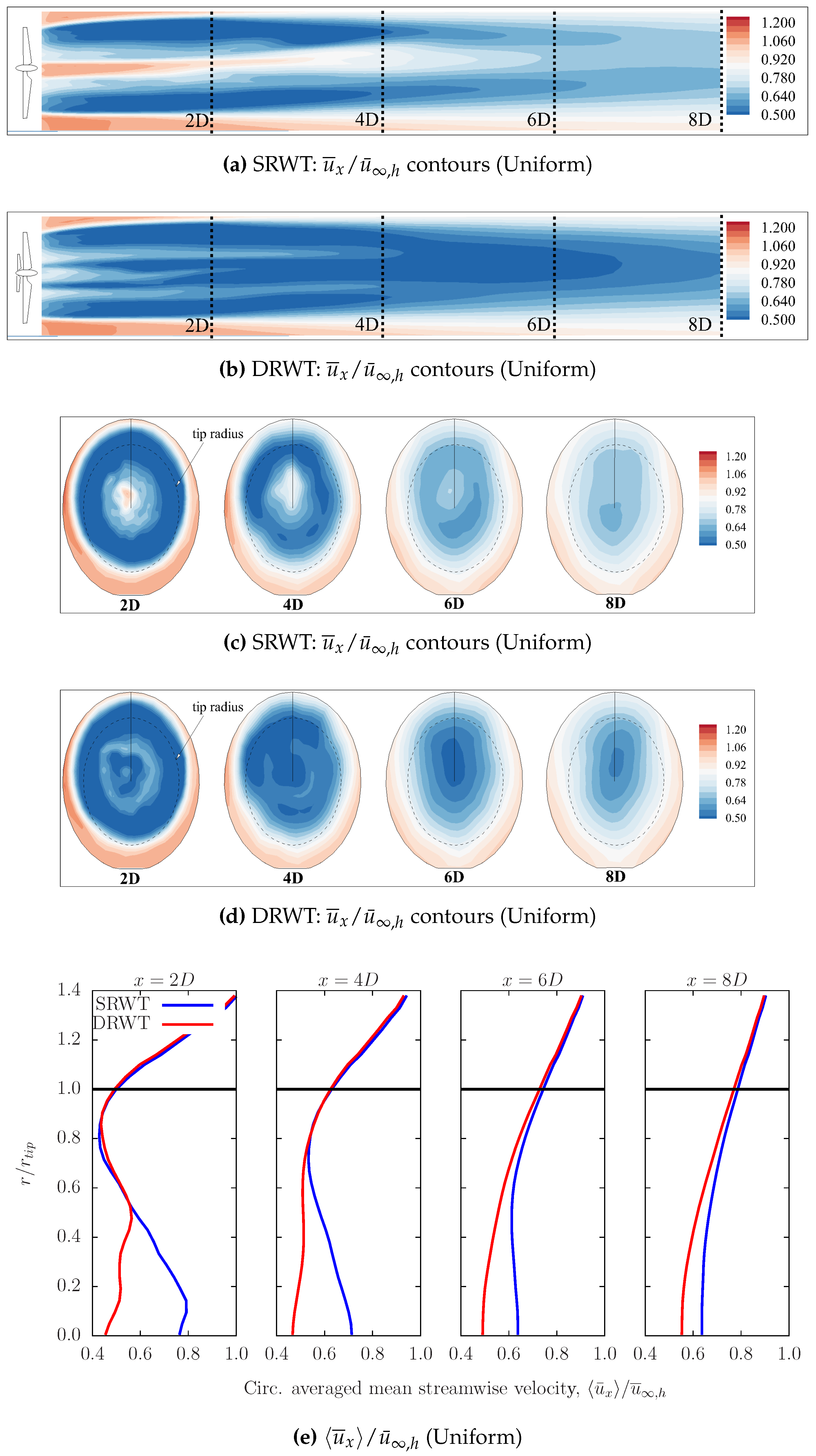
4.2.2. Turbine Wake Mixing
Mean Flow
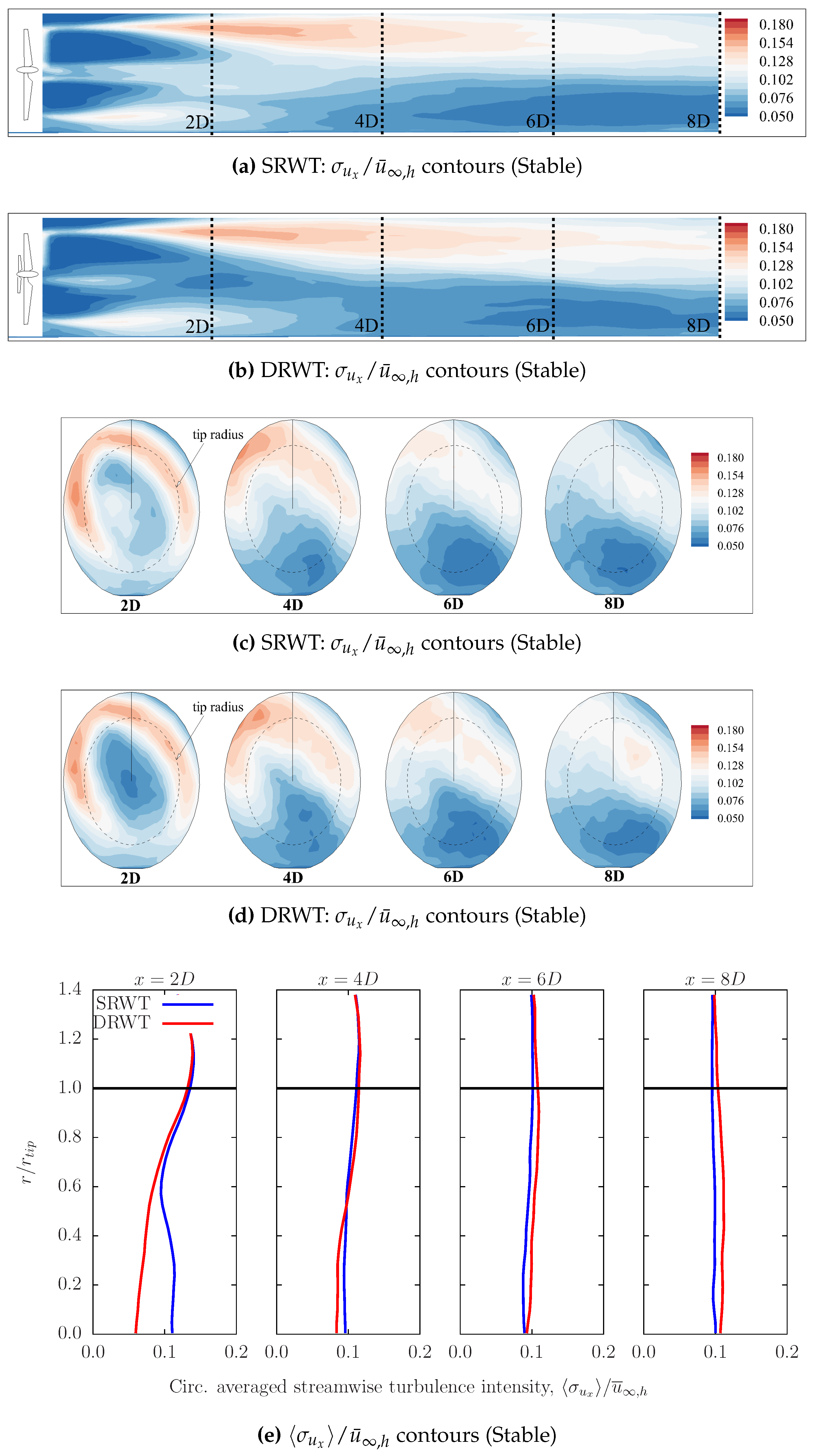
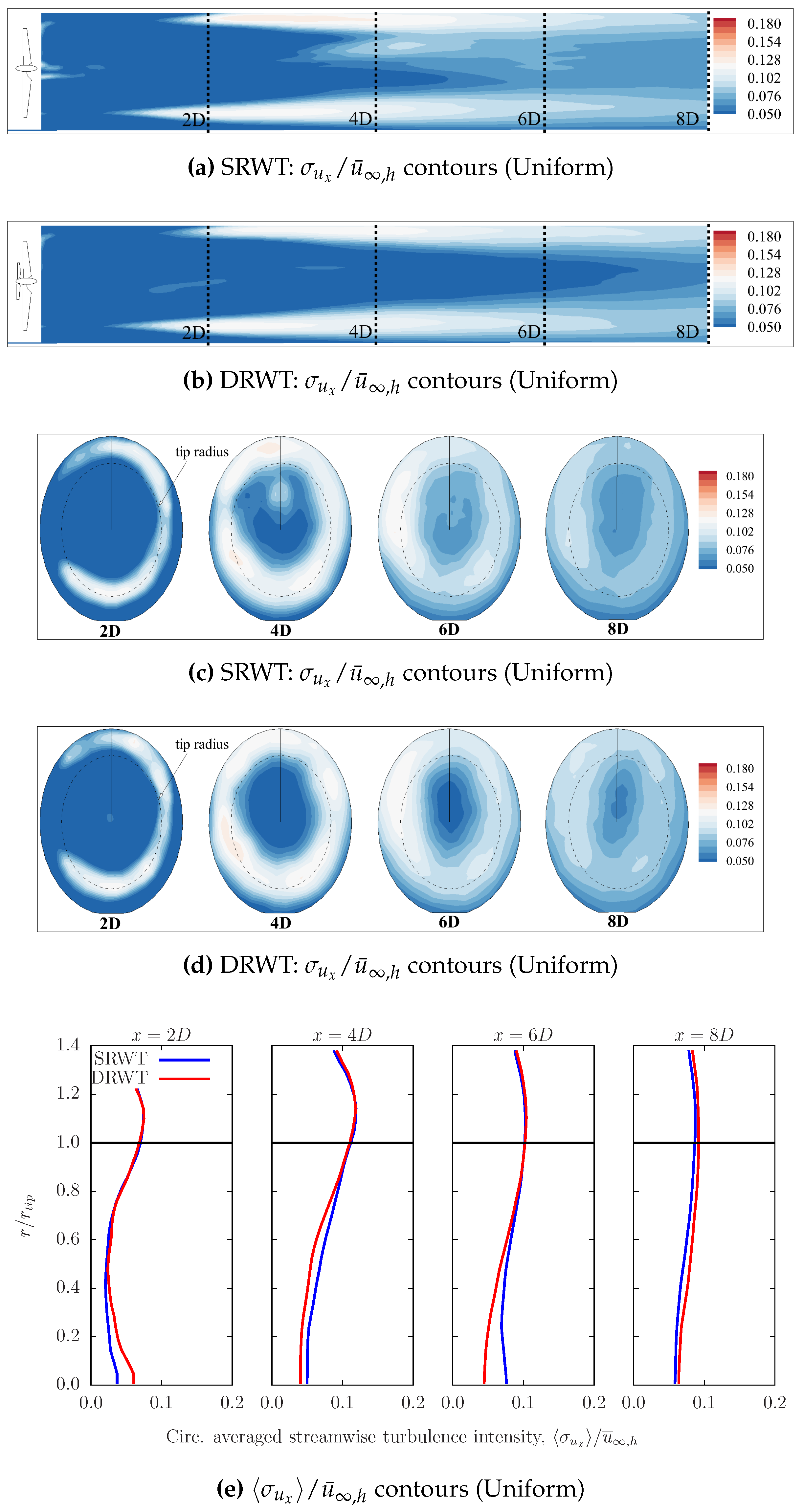
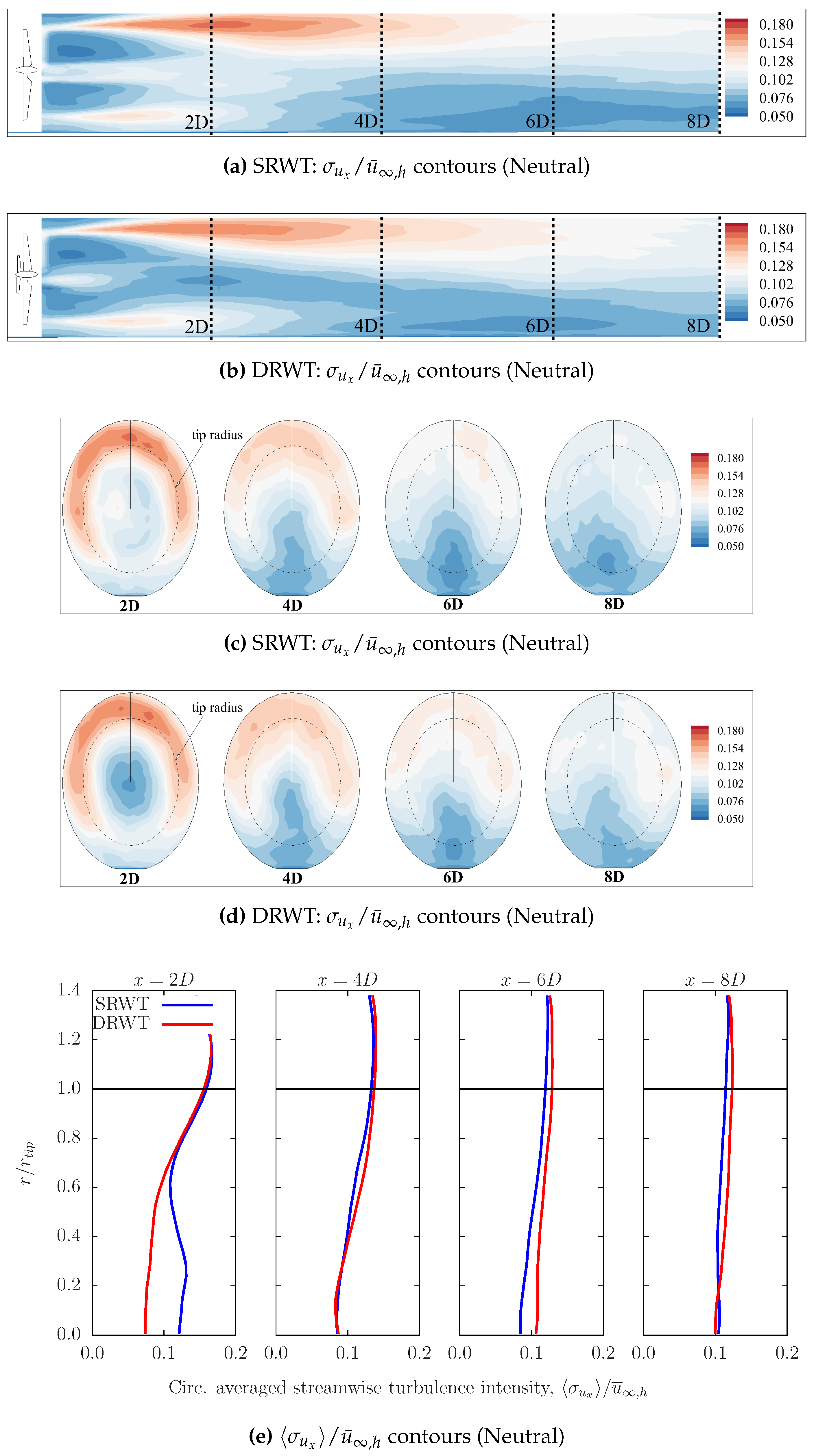
Turbulence Intensity
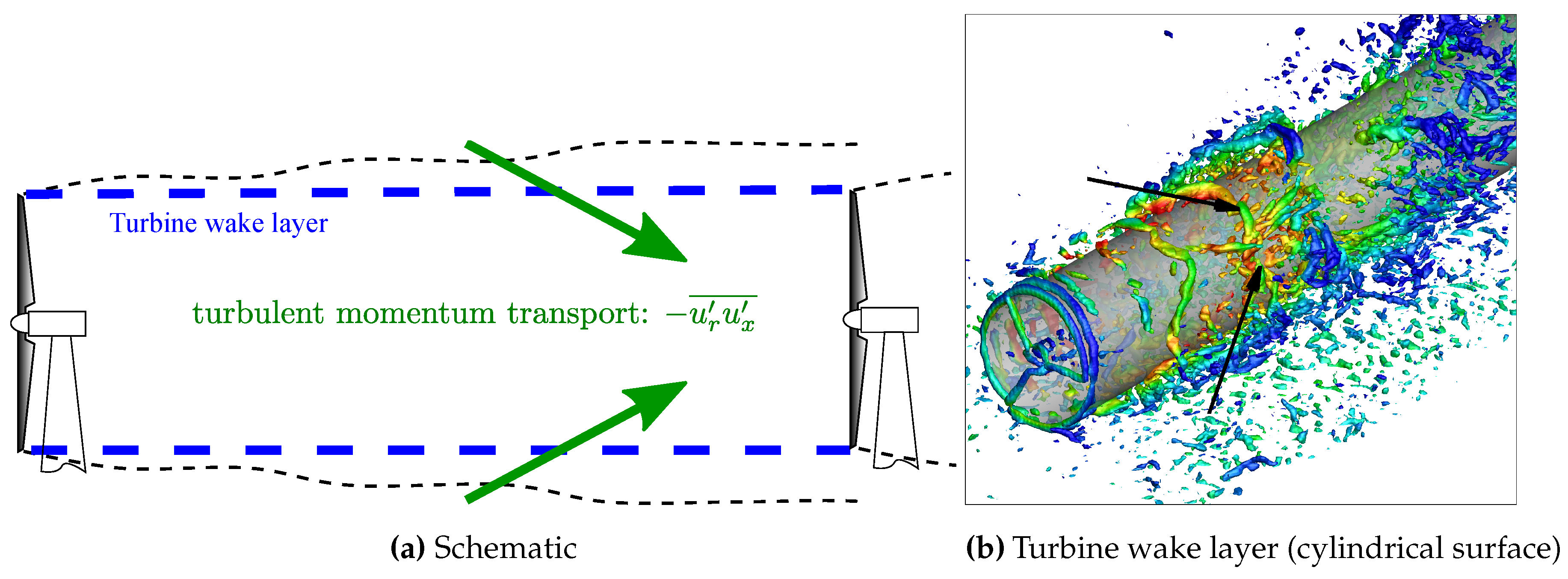
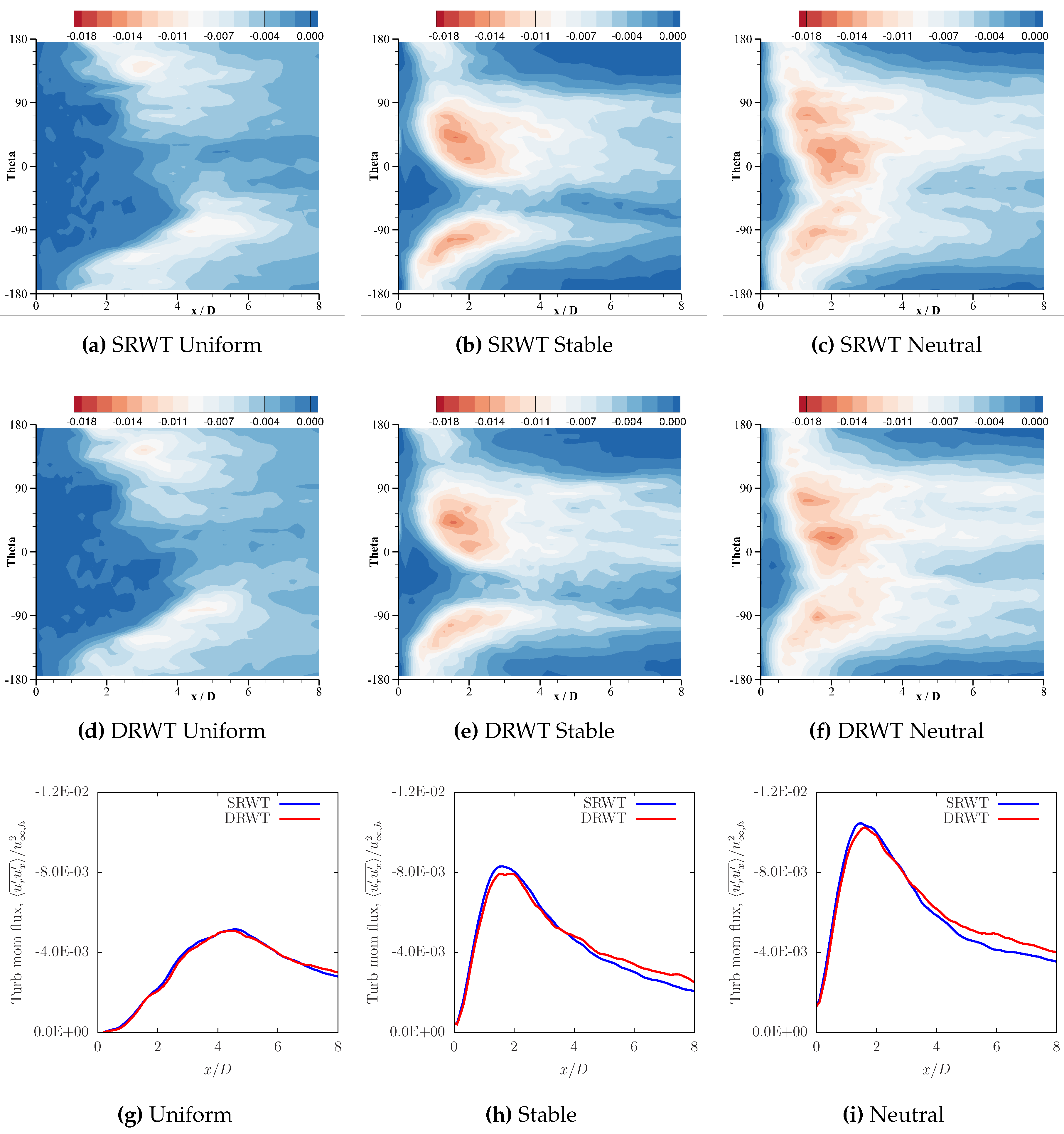
4.2.3. Momentum Entrainment
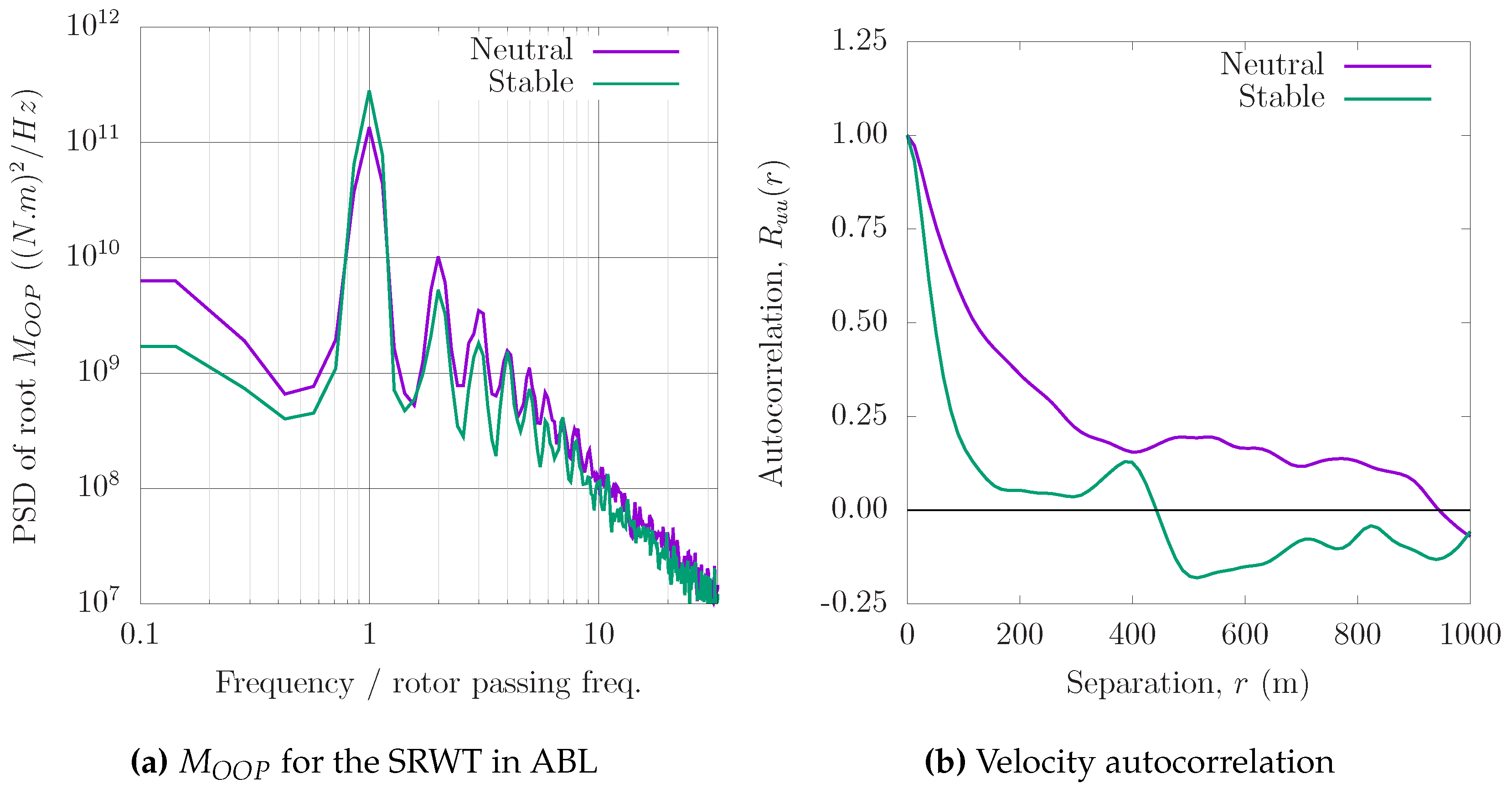
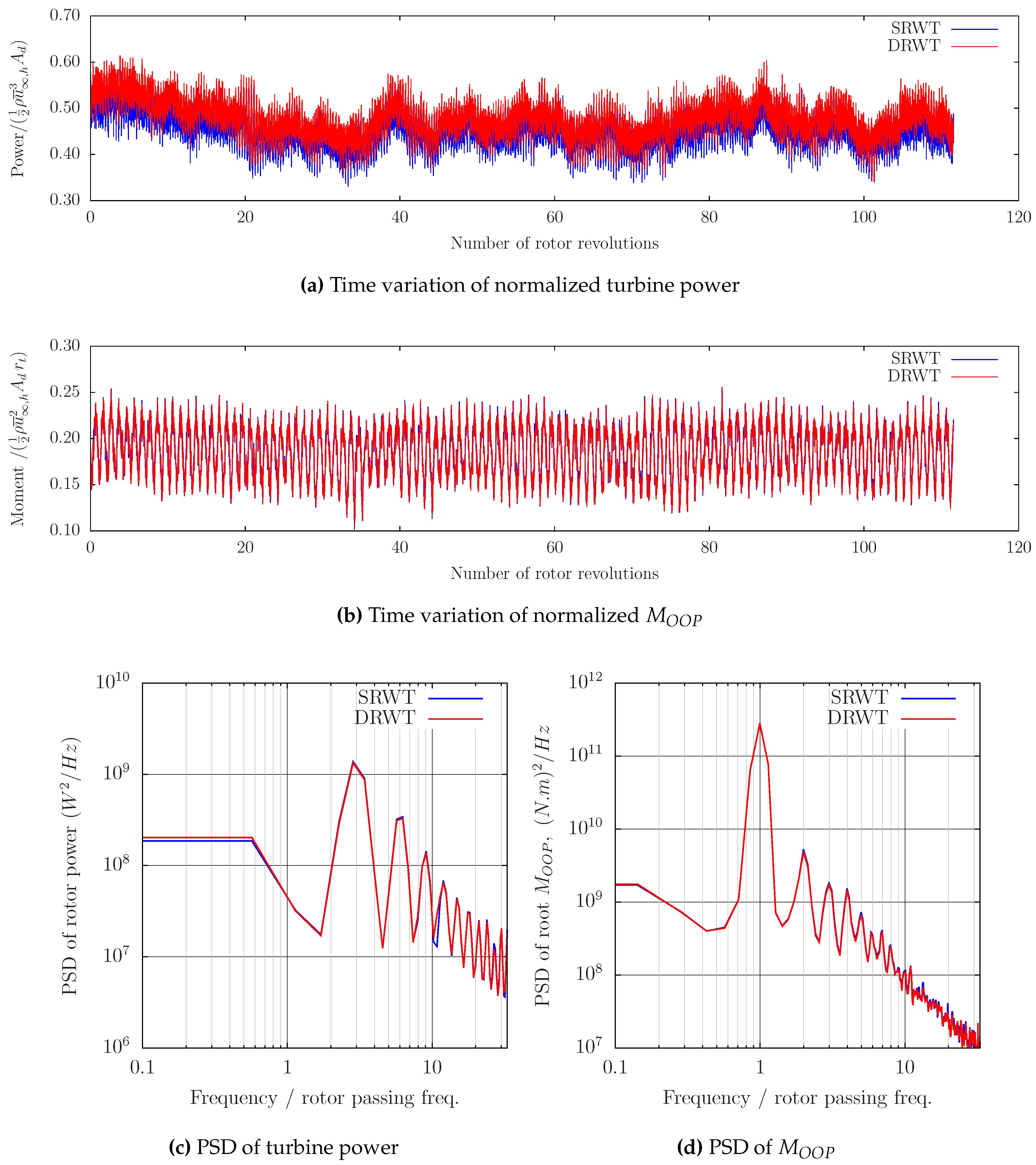
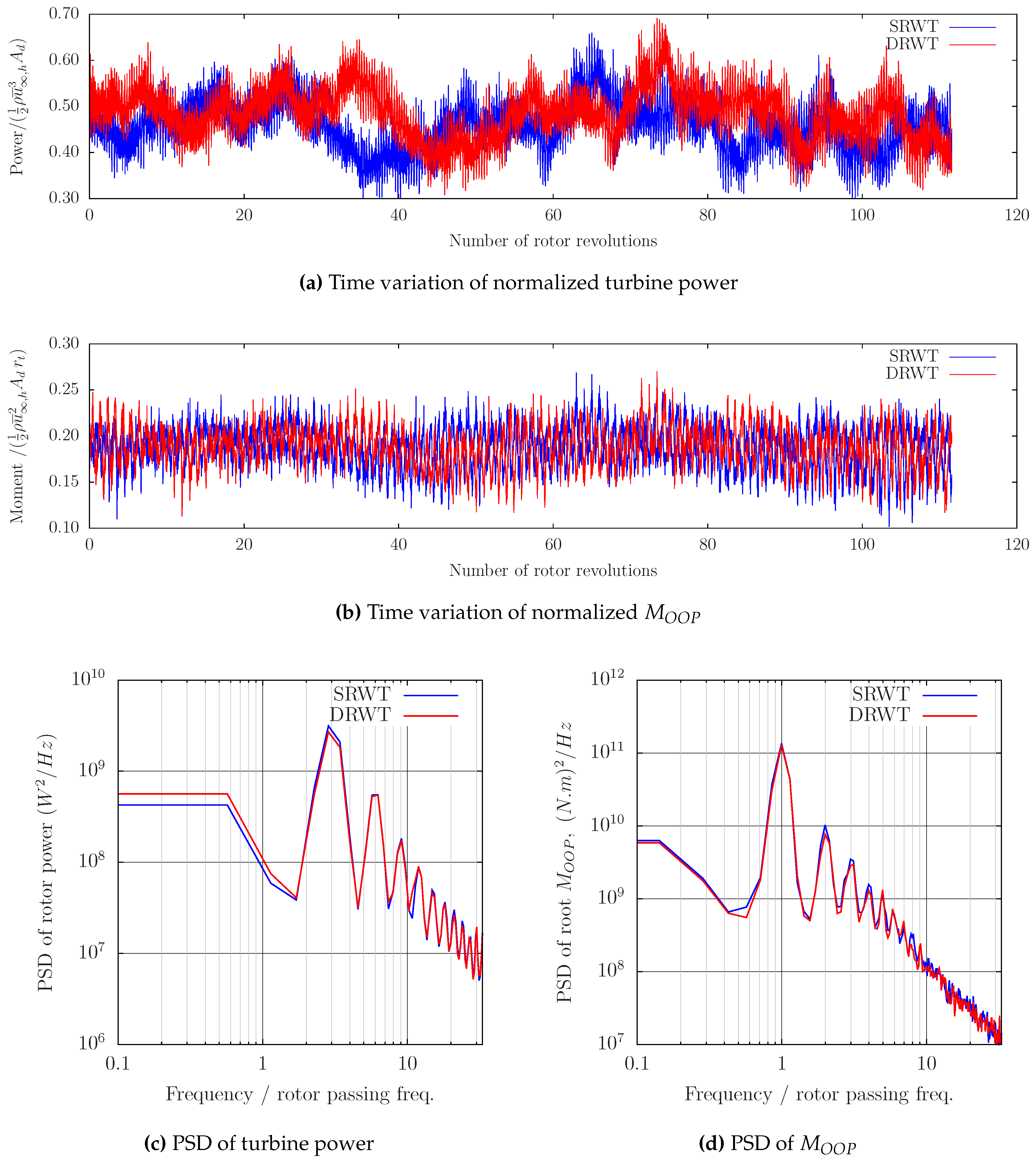
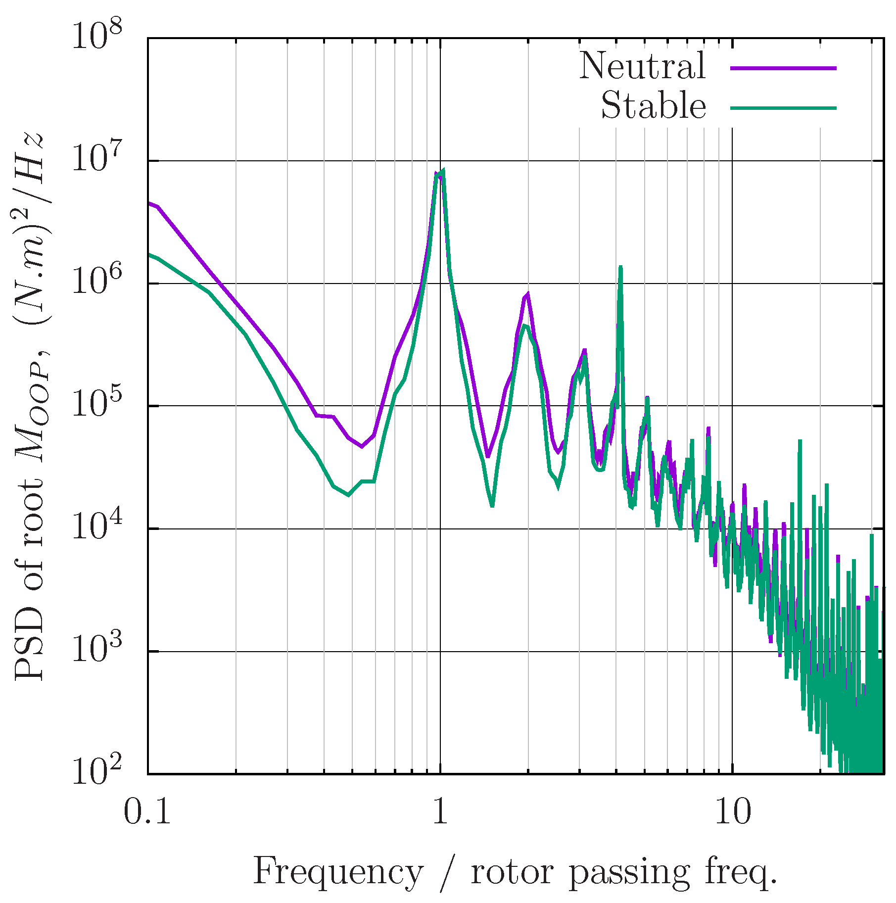
4.3. Aerodynamic Loads
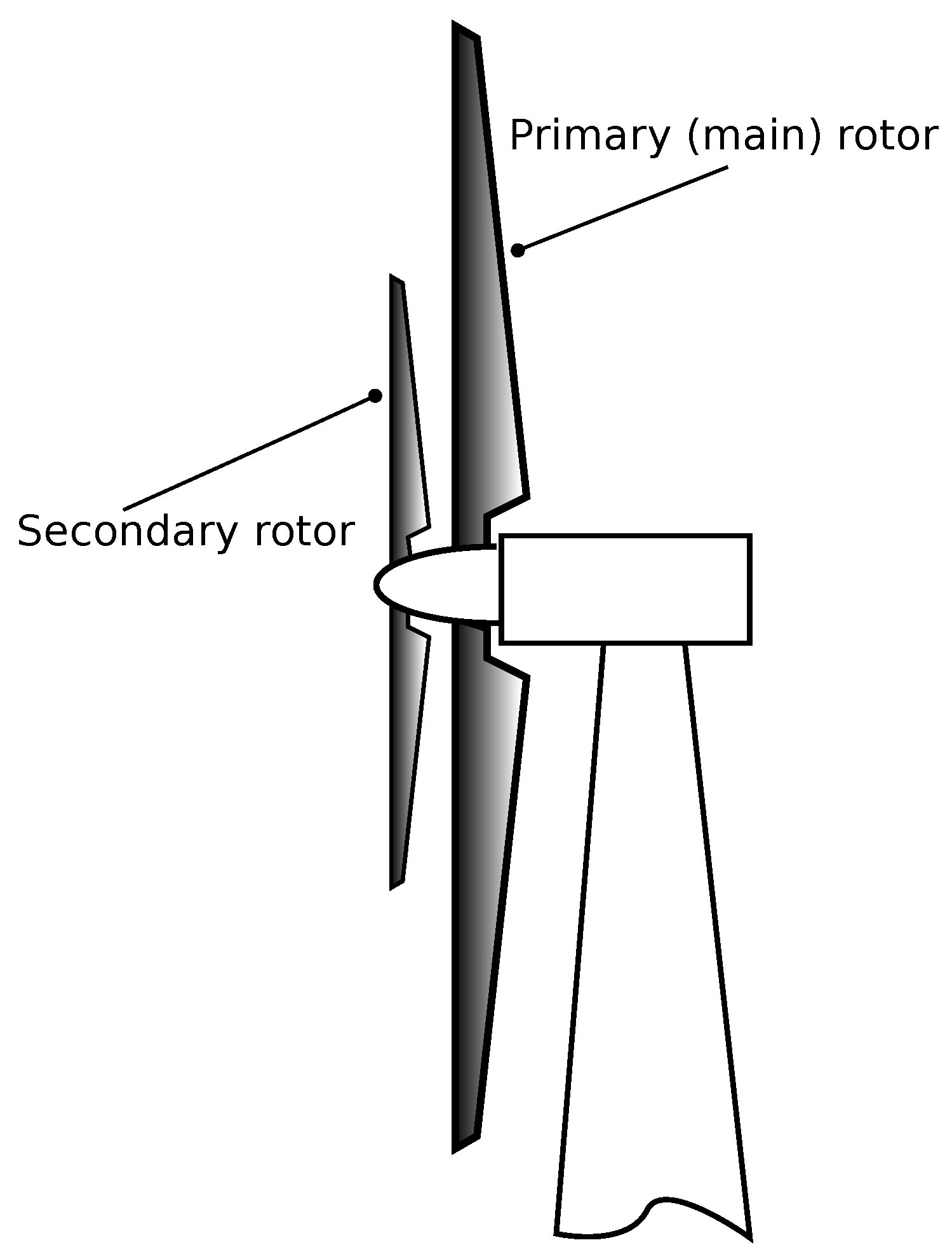
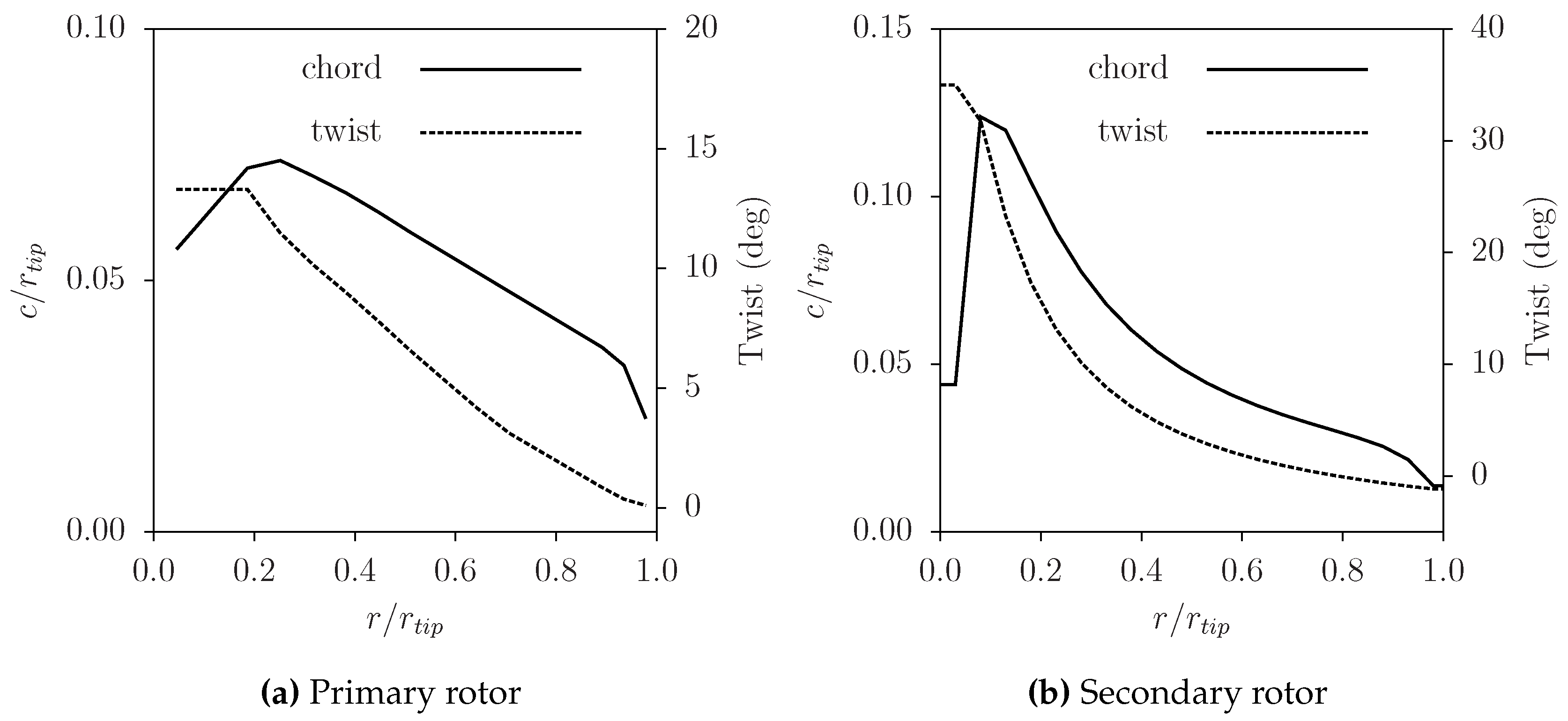
Secondary Rotor
5. Conclusions
- The DRWT operating in isolation shows aerodynamic performance () improvement of about 5%–6% for all inflow conditions. The performance benefit is obtained due to efficient extraction of energy (using the smaller secondary rotor) from the streamtube going through the blade root region.
- The DRWT enhances wake mixing and entrainment of higher momentum fluid from outside the wake layer when the atmospheric (freestream) turbulence is moderately high (as in the neutral stability case simulated here). A modest () increase in momentum entrainment is observed with the de facto DRWT design.
- The enhancement in wake mixing is associated with the increased turbulence intensity in the wake. This could potentially increase fatigue loads on the downstream turbines.
- Spectral analysis of aerodynamic loads (measured as rotor power and out-of-plane blade root moment) shows negligible reduction for the main rotor in the DRWT. Unsteady fluctuations in rotor power are observed at blade passing frequency, while fluctuations in blade root moments are at the rotor passing frequency and its harmonics. These fluctuations occur because of the azimuthal variation (due to the ABL) in the incoming mean wind, as well as turbulence in the wind.
Acknowledgments
Author Contributions
Conflicts of Interest
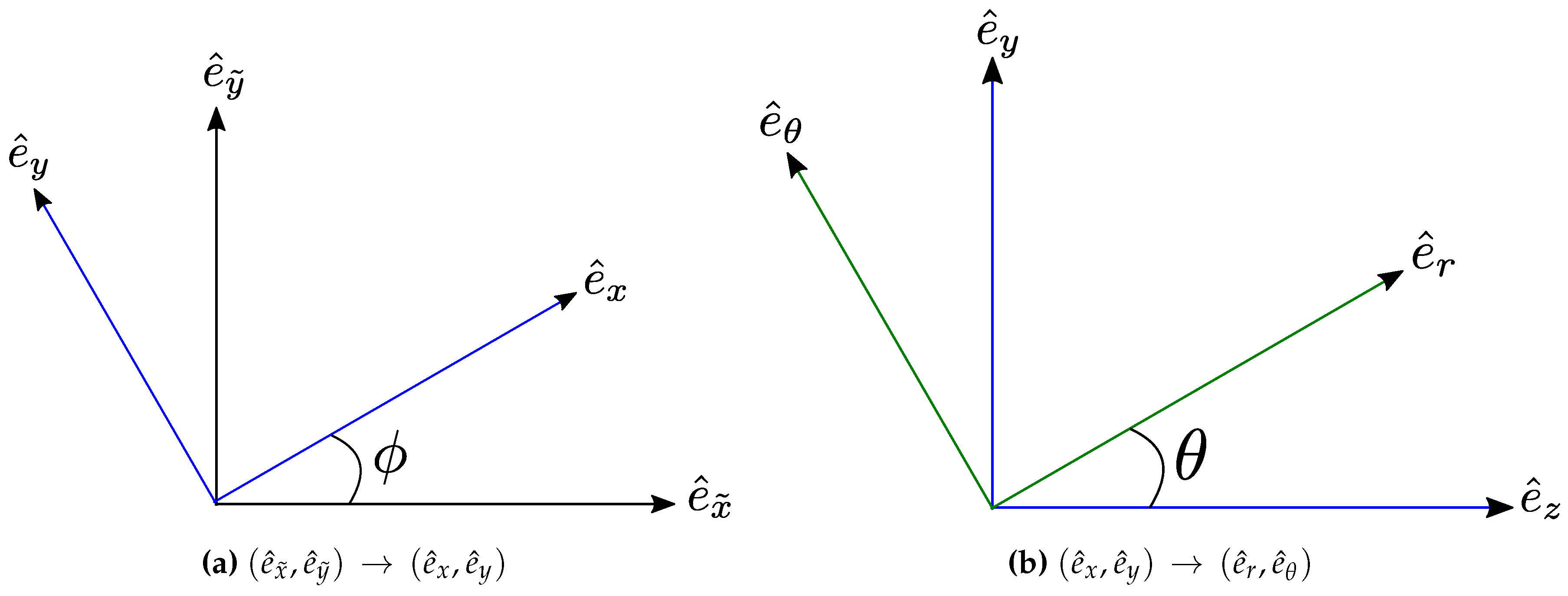
Appendix Coordinate Systems

Appendix A.1 Streamwise Turbulence Intensity
Appendix A.2 Streamwise Turbulent Momentum and Energy Flux
References
- Sharma, A.; Taghaddosi, F.; Gupta, A. Diagnosis of Aerodynamic Losses in the Root Region of a Horizontal Axis Wind Turbine; General Electric Company Technical Report; General Electric Global Research Center: Niskayuna, NY, USA, 2010. [Google Scholar]
- Barthelmie, R.J.; Jensen, L.E. Evaluation of power losses due to wind turbine wakes at the Nysted offshore wind farm. Wind Energy 2010, 13, 573–586. [Google Scholar] [CrossRef]
- Baker, J.; Mayda, E.; Van Dam, C. Experimental analysis of thick blunt trailing-edge wind turbine airfoils. J. Solar Energy Eng. 2006, 128, 422–431. [Google Scholar] [CrossRef]
- Fuglsang, P.; Bak, C. Development of the Risø Wind Turbine Airfoils. Wind Energy 2004, 7, 145–162. [Google Scholar] [CrossRef]
- Kusiak, A.; Song, Z. Design of wind farm layout for maximum wind energy capture. Renew. Energy 2010, 35, 685–694. [Google Scholar] [CrossRef]
- González, J.S.; Rodriguez, A.G.G.; Mora, J.C.; Santos, J.R.; Payan, M.B. Optimization of wind farm turbines layout using an evolutive algorithm. Renew. Energy 2010, 35, 1671–1681. [Google Scholar] [CrossRef]
- Mittal, P.; Kulkarni, K.; Mitra, K. A novel hybrid optimization methodology to optimize the total number and placement of wind turbines. Renew. Energy 2016, 86, 133–147. [Google Scholar] [CrossRef] [Green Version]
- Dabiri, J.O. Potential order-of-magnitude enhancement of wind farm power density via counter-rotating vertical-axis wind turbine arrays. J. Renew. Sustain. Energy 2011, 3, 043104. [Google Scholar] [CrossRef]
- Corten, G.P.; Lindenburg, K.; Schaak, P. Assembly of Energy Flow Collectors, Such as Windpark, and Method of Operation. U.S. Patent 7,299,627, 27 November 2007. [Google Scholar]
- Jiménez, Á.; Crespo, A.; Migoya, E. Application of a LES technique to characterize the wake deflection of a wind turbine in yaw. Wind energy 2010, 13, 559–572. [Google Scholar] [CrossRef]
- Westergaard, C.H. Method for Improving Large Array Wind Park Power Performance Through Active Wake Manipulation Reducing Shadow Effects. U.S. Patent App. 14/344,284, 21 March 2012. [Google Scholar]
- Newman, B. Multiple Actuator-Disc Theory for Wind Turbines. J. Wind Eng. Ind. Aerodyn. 1986, 24, 215–225. [Google Scholar] [CrossRef]
- Jung, S.N.; No, T.S.; Ryu, K.W. Aerodynamic performance prediction of a 30kW counter-rotating wind turbine system. Renew. Energy 2005, 30, 631–644. [Google Scholar] [CrossRef]
- Kanemoto, T.; Galal, A.M. Development of intelligent wind turbine generator with tandem wind rotors and double rotational armatures (1st report, superior operation of tandem wind rotors). JSME Int. J. Ser. B 2006, 49, 450–457. [Google Scholar] [CrossRef]
- Kanemoto, T. Wind Turbine Generator. U.S. Patent App. 13/147,021, 19 April 2010. [Google Scholar]
- Rosenberg, A.; Selvaraj, S.; Sharma, A. A Novel Dual-Rotor Turbine for Increased Wind Energy Capture. J. Phys. Conf. Ser. 2014, 524, 012078. [Google Scholar] [CrossRef]
- Rosenberg, A.; Sharma, A. A Prescribed-Wake Vortex Lattice Method for Aerodynamic Analysis and Optimization of Co-Axial, Dual-Rotor Wind Turbines. ASME J. Solar Energy Eng. 2016. submitted. [Google Scholar]
- Selvaraj, S. Numerical Investigation of Wind Turbine and Wind Farm Aerodynamics. Master’s Thesis, Iowa State University, Ames, IA, USA, 2014. [Google Scholar]
- Jonkman, J.; Butterfield, S.; Musial, W.; Scott, G. Definition of a 5-MW Reference Wind Turbine for Offshore System Development; NREL: Golden, CO, USA, 2009. [Google Scholar]
- Mikkelsen, R. Actuator Disk Models Applied to Wind Turbines. Ph.D. Thesis, Technical University of Denmark, Copenhagen, Denmark, 2003. [Google Scholar]
- Betz, A. Schraubenpropeller mit Geringstem Energieverlust. Nachrichten von der Gesellschaft der Wissenschafte n zu Göttingen, Mathematisch-Physikalische Klasse 1919, 193–217. [Google Scholar]
- Goldstein, S. On the vortex theory of screw propellers. R. Soc. 1929, 123, 440–465. [Google Scholar] [CrossRef]
- Burton, T.; Sharpe, D.; Jenkins, N.; Bossanyi, E. Wind Energy Handbook; John Wiley & Sons Ltd.: Chichester, UK, 2002. [Google Scholar]
- Ainslie, J.F. Calculating the Flow Field in the Wake of Wind Turbines. J. Wind Eng. Ind. Aerodyn. 1988, 27, 213–224. [Google Scholar] [CrossRef]
- Snel, H. Review of Aerodynamics for Wind Turbines. Wind Energy 2003, 6, 203–211. [Google Scholar] [CrossRef]
- Calaf, M.; Meneveau, C.; Meyers, J. Large eddy simulation study of fully developed wind-turbine array boundary layers. Phys. Fluids 2010, 22, 015110. [Google Scholar] [CrossRef]
- Vermeer, L.J.; Sørensen, J.N.; Crespo, A. Wind Turbine Wake Aerodynamics. Prog. Aerosp. Sci. 2003, 39, 467–510. [Google Scholar] [CrossRef]
- Sanderse, B.; van der Pijl, S.P.; Koren, B. Review of Computational Fluids Dynamics for Wind Turbine Wake Aerodynamics. Wind Energy 2011. [Google Scholar] [CrossRef]
- Jimenez, A.; Crespo, A.; Migoya, E.; Garcia, J. Advances in Large-Eddy Simulation of a Wind Turbine Wake. J. Phys. Conf. Ser. 2007, 75, 015004. [Google Scholar] [CrossRef]
- Jimenez, A.; Crespo, A.; Migoya, E.; Garica, J. Large Eddy Simulation of Spectral Coherence in a Wind Turbine Wake. Environ. Res. Lett. 2008, 3, 015004. [Google Scholar] [CrossRef]
- Porté-Agel, F.; Wu, Y.; Lu, H.; Conzemius, R.J. Large-Eddy Simulation of Atmospheric Boundary Layer Flow through Wind Turbines and Wind Farms. J. Wind Eng. Ind. Aerodyn. 2011, 99, 154–168. [Google Scholar] [CrossRef]
- Wu, Y.; Porté-Agel, F. Large-Eddy Simulation of Wind-Turbine Wakes: Evaluation of Turbine Parametrisations. Bound. Layer Meteorol. 2011, 138, 345–366. [Google Scholar] [CrossRef]
- Troldborg, N.; Larsen, G.C.; Madsen, H.A.; Hansen, K.S.; Sørensen, J.N.; Mikkelsen, R. Numerical simulations of wake interaction between two wind turbines at various inflow conditions. Wind Energy 2011, 14, 859–876. [Google Scholar] [CrossRef]
- Porté-Agel, F.; Wu, Y.T.; Chen, C.H. A numerical study of the effects of wind direction on turbine wakes and power losses in a large wind farm. Energies 2013, 6, 5297–5313. [Google Scholar] [CrossRef]
- Stevens, R.J.; Gayme, D.F.; Meneveau, C. Large eddy simulation studies of the effects of alignment and wind farm length. J. Renew. Sustain. Energy 2014, 6, 023105. [Google Scholar] [CrossRef]
- Churchfield, M.J.; Lee, S.; Michalakes, J.; Moriarty, P.J. A numerical study of the effects of atmospheric and wake turbulence on wind turbine dynamics. J. Turbul. 2012, 13, 1–32. [Google Scholar] [CrossRef]
- Churchfield, M.; Lee, S.; Moriarty, P. A Large-Eddy Simulation of Wind-Plant Aerodynamics. In Proceedings of the 50th AIAA Aerospace Sciences Meeting including the New Horizons Forum and Aerospace Exposition, Nashville, TN, USA, 9–12 January 2012; 2012. [Google Scholar]
- Smagorinsky, J. General Circulation Experiments with the Primitive Equations I. The Basic Experiment. Monthly Weather Rev. 1963, 91, 99–164. [Google Scholar] [CrossRef]
- Lilly, D.K. A proposed modification of the Germano subgrid-scale closure method. Phys. Fluids A Fluid Dyn. (1989–1993) 1992, 4, 633–635. [Google Scholar] [CrossRef]
- Germano, M.; Piomelli, U.; Moin, P.; Cabot, W.H. A dynamic subgrid-scale eddy viscosity model. Phys. Fluids A Fluid Dyn. (1989–1993) 1991, 3, 1760–1765. [Google Scholar] [CrossRef]
- Churchfield, M.; Lee, S. NWTC Design Codes (SOWFA). Available online: http://wind.nrel.gov/designcodes/simulators/SOWFA (accessed on 6 July 2016).
- Moeng, C. A Large-Eddy-Simulation Model for the Study of Planetary Boundary-Layer Turbulence. J. Atmosp. Sci. 1984, 41, 2052–2062. [Google Scholar] [CrossRef]
- Stull, R.B. An Introduction to Boundary Layer Meteorology; Kluwer Academic Publishers: Dordecht, The Netherlands, 1988. [Google Scholar]
- Lee, S.; Churchfield, M.; Moriarty, P.; Jonkman, J.; Michalakes, J. Atmospheric and wake turbulence impacts on wind turbine fatigue loadings. AIAA Paper 2012-0540; 2012. Available online: http://www.nrel.gov/docs/fy12osti/53567.pdf (accessed on 21 July 2016). [Google Scholar]
- Jonkman, J.; Buhl, M. FAST User’s Guide; NREL Technical Report No. NREL/EL-500-38230; National Renewable Energy Laboratory: Golden, CO, USA, 2005.
- Schepers, J.; Brand, A.; Bruining, A.; Graham, J.; Hand, M.; Infield, D.; Madsen, H.; Paynter, R.; Simms, D. Final Report of IEA Annex XIV: Field Rotor Aerodynamics; Technical Report ECN-C-97-027; Energy Research Center of the Netherlands: Petten, The Netherlands, 1997. [Google Scholar]
- Organization, W.M. Guide to Meteorological Instruments and Methods of Observation; Secretariat of the World Meteorological Organization: Geneva, Switzerland, 1983. [Google Scholar]
- Davidson, L. HYBRID LES-RANS: Inlet Boundary Conditions for Flows with Recirculation. In Advances in Hybrid RANS-LES Modelling; Springer: Berlin, Germany, 2008; pp. 55–66. [Google Scholar]
- Sedefian, L.; Bennett, E. A comparison of turbulence classification schemes. Atmosp. Environ. (1967) 1980, 14, 741–750. [Google Scholar] [CrossRef]
- Businger, J.A. Turbulent transfer in the atmospheric surface layer. Q. J. R. Meteorol. Soc. 1972, 98, 67–100. [Google Scholar]
- Chamorro, L.P.; Porté-Agel, F. Effects of thermal stability and incoming boundary-layer flow characteristics on wind-turbine wakes: A wind-tunnel study. Bound. Layer Meteorol. 2010, 136, 515–533. [Google Scholar] [CrossRef]
- Jha, P.K.; Duque, E.P.; Bashioum, J.L.; Schmitz, S. Unraveling the Mysteries of Turbulence Transport in a Wind Farm. Energies 2015, 8, 6468–6496. [Google Scholar] [CrossRef]
- Chamorro, L.; Guala, M.; Arndt, R.; Sotiropoulos, F. On the evolution of turbulent scales in the wake of a wind turbine model. J. Turbul. 2012, 13. [Google Scholar] [CrossRef]
- Cal, R.B.; Lebrón, J.; Castillo, L.; Kang, H.S.; Meneveau, C. Experimental study of the horizontally averaged flow structure in a model wind-turbine array boundary layer. J. Renew. Sustain. Energy 2010, 2, 013106. [Google Scholar] [CrossRef]
- Wu, Y.T.; Porté-Agel, F. Large-eddy simulation of wind-turbine wakes: Evaluation of turbine parametrisations. Bound. Layer Meteorol. 2011, 138, 345–366. [Google Scholar] [CrossRef]


| Case | %ΔPower | % |
|---|---|---|
| Uniform inflow | 5.0 | −0.39 |
| Stable ABL | 5.4 | −0.29 |
| Neutral ABL | 6.1 | −0.07 |
| Inflow Condition | ||
|---|---|---|
| Uniform | −1.17% | −2.30% |
| Stable | +1.78% | +1.63% |
| Neutral | +3.29% | +2.54% |
© 2016 by the authors; licensee MDPI, Basel, Switzerland. This article is an open access article distributed under the terms and conditions of the Creative Commons Attribution (CC-BY) license (http://creativecommons.org/licenses/by/4.0/).
Share and Cite
Moghadassian, B.; Rosenberg, A.; Sharma, A. Numerical Investigation of Aerodynamic Performance and Loads of a Novel Dual Rotor Wind Turbine. Energies 2016, 9, 571. https://doi.org/10.3390/en9070571
Moghadassian B, Rosenberg A, Sharma A. Numerical Investigation of Aerodynamic Performance and Loads of a Novel Dual Rotor Wind Turbine. Energies. 2016; 9(7):571. https://doi.org/10.3390/en9070571
Chicago/Turabian StyleMoghadassian, Behnam, Aaron Rosenberg, and Anupam Sharma. 2016. "Numerical Investigation of Aerodynamic Performance and Loads of a Novel Dual Rotor Wind Turbine" Energies 9, no. 7: 571. https://doi.org/10.3390/en9070571