Risk Assessment of Distribution Networks Considering the Charging-Discharging Behaviors of Electric Vehicles

Abstract

Electric vehicles (EVs) have received wide attention due to their higher energy efficiency and lower emissions. However, the random charging and discharging behaviors of substantial numbers of EVs may lead to safety risk problems in a distribution network. Reasonable price incentives can guide EVs through orderly charging and discharging, and further provide a feasible solution to reduce the operational risk of the distribution network. Considering three typical electricity prices, EV charging/discharging load models are built. Then, a Probabilistic Load Flow (PLF) method using cumulants and Gram-Charlier series is proposed to obtain the power flow of the distribution network including massive numbers of EVs. In terms of the risk indexes of node voltage and line flow, the operational risk of the distribution network can be estimated in detail. From the simulations of an IEEE-33 bus system and an IEEE 69-bus system, the demonstrated results show that reasonable charging and discharging prices are conducive to reducing the peak-valley difference, and consequently the risks of the distribution network can be decreased to a certain extent.

1. Introduction

With the increasing concern about environmental pollution and fossil energy shortage, EVs are becoming an important alternative means of transport due to their higher energy efficiency and lower emissions compared with conventional internal combustion engine (ICE) vehicles. In this situation, the EV industry is booming due to the incentives of government policies and market requirements [1]. However, regarding when all those EVs are connected to the distribution network, the uncertainties of the charging and discharging demands could lead to risks in the safety of the distribution network [2,3]. In a way, scientific and effective risk assessment is conducive to ensure the safe and stable operation of the power system. Therefore, it is significant to study the operational risk assessment of substantial numbers of EVs’ charging and discharging behaviors on the distribution system.

Large-scale unordered charging demand of EVs [4,5], however, is more likely to coincide with the overall peak load, which would make the node voltage and line flow exceed the acceptable ranges [6,7,8]. References [9,10,11] comprehensively analyze the impacts of EVs on distribution networks, while coordinated EV scheduling methods [12,13] could reduce those adverse effects. Note that, EV owners are able to actively adjust the charging or discharging time in accordance with variable electricity prices. Hence, a reasonable price incentive mechanism is necessary to guide the charging and discharging behaviors of EVs [14,15,16], which could shift the peak load and reduce the safety risks of the power grid. References [17,18,19] introduce an EV charging model based on the time-of-use (TOU) price, and the EV charging load can be shifted from peak load hours to off-peak load hours. However, few works focus on the discharging price of EV. Considering Vehicle to Grid (V2G) technology [20,21], EVs can reverse discharge to the power system, which plays a very significant role in “cut peak and fill valley”, and further the operational risks may be potentially reduced. Gao et al. [22] preliminarily studied EVs’ power demands where the discharging price is selectively included, but the impact of the EVs on the operation of power grid under different prices is not taken into account.

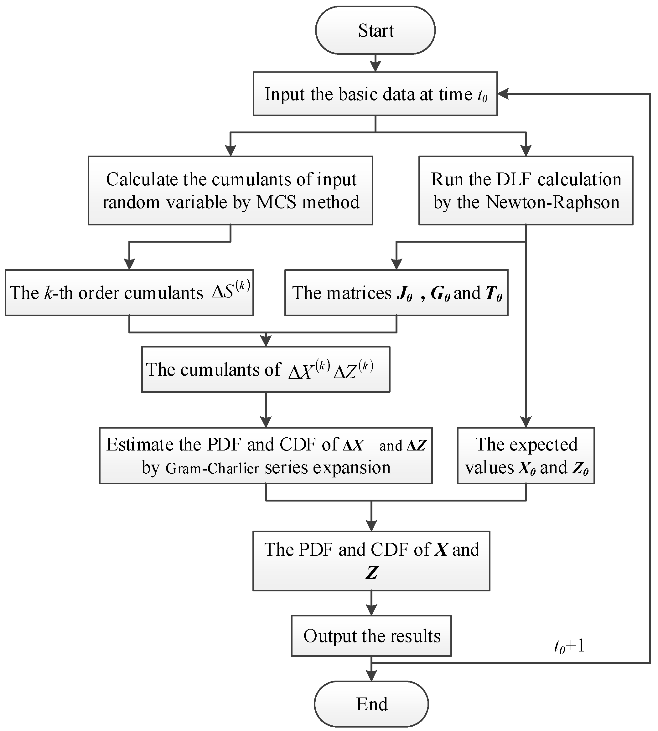
The uncertainties of substantial numbers EVs will result in a significant change in the power flow distribution, and unstable operation of the distribution network may be caused. The Probabilistic Load Flow (PLF) calculation method using cumulants and Gram-Charlier series [23,24] can quickly calculate the probability density function (PDF) and cumulative distribution function (CDF) of state variables, which can provide the basic data for the calculation of risk assessment. Further, the operational risk assessment can comprehensively measure the possibility and severity of uncertainties [25]. In consideration of randomness and fuzziness, Feng et al. [26] presents a risk assessment method to deal with the two-fold uncertainty. Deng et al. [27] introduces the conditional value-at-risk (CVaR) to a risk-based security assessment method considering future conditions. Hu [28] proposes a risk assessment method for distribution network integrated with wind power and EVs, but this study does not involve the discharging characteristics of EVs.

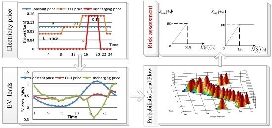
Considering EVs’ charging and discharging behaviors, this paper proposes a risk assessment method to evaluate the operational risks of distribution network, and also the assessment method’s performance is studied under different simulation cases. The paper is organized in the following manner: in Section 2, the EV charging/discharging demand models corresponding to different electricity prices are built. Section 3 conducts a dynamic PLF method using cumulants and Gram-Charlier. In Section 4, a calculation method of risk assessment on distribution network is proposed. In Section 5, numerical simulations are carried out in an IEEE 33-bus system and an IEEE 69-bus system, respectively. In Section 6, conclusions are summarized and next steps are suggested.

2. The EV Charging/Discharging Load Models under Different Electricity Prices

A reasonable price incentive is conducive to managing the charging and discharging power loads of EVs. In this section, the slow charging household EVs are studied, and herein three load models for EV charging/discharging are established based on typical electricity prices, including the constant electricity price, the ordinary TOU price and the improved TOU price, respectively.

2.1. The Unordered Charging Load Model under Constant Price

It is assumed that EVs have similar driving characteristics as conventional ICE vehicles. According to the National Household Travel Survey (NHTS) conducted by the US Department of Transportation [29], the probability density functions of the home arrival time and the daily driving distance can be respectively obtained by use of the normalization and maximum likelihood parameter estimation method.

(1)

Home arrival time

It is assumed that most users will charge their EVs once they return home from work without relevant regulations and price stimulus. The probability density function of the start time of charging [29], which is considered to be normally distributed, is denoted as follows.

$$f_s\left(x\right)=\{\begin{array}{ll}\frac{1}{{\mathsf{\sigma }}_s\sqrt{2\mathsf{\pi }}}{\mathrm{e}}^{\frac{-{\left(x-{\mathsf{\mu }}_s\right)}^2}{2{{\mathsf{\sigma }}_s}^2}}& \left({\mathsf{\mu }}_s-12\right)<x\le 24\\ \frac{1}{{\mathsf{\sigma }}_s\sqrt{2\mathsf{\pi }}}{\mathrm{e}}^{\frac{-{\left(x+24-{\mathsf{\mu }}_s\right)}^2}{2{{\mathsf{\sigma }}_s}^2}}& 0<x\le \left({\mathsf{\mu }}_s-12\right)\end{array}$$

(1)

where x is the start time of charging, μ_s = 17.6 and σ_s = 3.4.

(2)

Daily driving distance

Daily driving distance represents the electricity consumption of an EV in a single day. The probability density function of the daily driving distance [29], which is considered to be log-normally distributed, is expressed as:

$$f_D\left(x\right)=\frac{1}{x{\mathsf{\sigma }}_D\sqrt{2\mathsf{\pi }}}{\mathrm{e}}^{\frac{-{\left(\text{ln}x-{\mathsf{\mu }}_D\right)}^2}{2{{\mathsf{\sigma }}_D}^2}}$$

(2)

where x is the daily driving distance, μ_D = 3.2 and σ_D = 0.88.

The duration time of charging for a certain EV can be obtained by:

$$T_c=\frac{D{W}_{100}}{100P_c}$$

(3)

where D is the daily traveling distance. W₁₀₀ represents the energy consumption per 100 kilometers. The term P_c is the charging power of EVs, and herein it is supposed to be unchangeable.

The probability density function of the charging time is denoted as:

$$f_{T_c}\left(x\right)=\frac{1}{x{\mathsf{\sigma }}_d\sqrt{2\mathsf{\pi }}}\text{exp}\left[\frac{-{\left(\text{ln}x+\text{ln}{P}_c-\text{ln}{W}_{100}-{\mathsf{\mu }}_d\right)}^2}{2{{\mathsf{\sigma }}_d}^2}\right]$$

(4)

(3)

The distribution model of EVs’ charging power

When the total number of EVs in the system is N, the amount of EVs which begin to charge from time i to time i + 1can be expressed as:

$$N_i^0={\displaystyle {\int }_i^{i+1}N\cdot f_s}\left(x\right)dx, \left(i=1,2\dots 24\right)$$

(5)

To simplify the analysis, the start time of EV charging is taken as the nearest smaller integer in this paper.

Most EVs can be fully charged in 16 h [5]. Therefore, the number of EVs which start charging at time i and lasting for k hours can be expressed as:

$$N_{ik}^0={\displaystyle {\int }_{k-1}^k{N}_i^0}\cdot f_{T_c}\left(x\right)dx, \left(k=1,2\dots 16\right)$$

(6)

2.2. The Charging Load Model under the Ordinary TOU Price

In general, the out-of-order charging of EVs may lead to serious overloading. The ordinary TOU price mechanism can be used to guide the EV owners’ charging behavior to optimize the EV loads.

(1)

The model of TOU price

According to the daily load curve, the ordinary TOU price divides the 24-h of a day into different periods. The electricity price at time t is denoted as:

$$f_{\mathsf{\rho }}\left(t\right)=\{\begin{array}{l}{\mathsf{\rho }}_P, t_{d1}\le t\le t_{d2}\\ {\mathsf{\rho }}_v, t_{c1}\le t\le t_{c2}\\ {\mathsf{\rho }}_f, \text{others}\end{array}$$

(7)

where ${\mathsf{\rho }}_p,{\mathsf{\rho }}_v,{\mathsf{\rho }}_n$ denote the price in peak, valley and flat time, respectively. [$t_{d_1}, t_{d_2}$], [$t_{c_1},t_{c_2}$] represent the peak and valley load period, respectively.

(2)

The response model of EVs considering the ordinary TOU price

The charging demand is directly affected by the electricity price. The price’s elasticity coefficient which reflects the demand response to price is expressed as:

$$\mathsf{\epsilon }=\frac{\Delta d/d_0}{\Delta \mathsf{\rho }/{\mathsf{\rho }}_0}$$

(8)

where d₀ and ${\mathsf{\rho }}_0$ represent the basic demand and price, respectively. $\Delta d$ and $\Delta \mathsf{\rho }$ refer to the changes in demand and price, respectively.

The demand at a certain time is not only affected by the price of the current time but also by the prices of other time. Thus, the self-elasticity coefficient and the cross-elasticity coefficient can be written as:

$$\begin{array}{l}{\epsilon }_{ii}=\frac{\Delta d_i/d_0}{\Delta {\mathsf{\rho }}_i/{\mathsf{\rho }}_0}\\ {\mathsf{\epsilon }}_{ij}=\frac{\Delta d_i/d_0}{\Delta {\mathsf{\rho }}_j/{\mathsf{\rho }}_0}\end{array}$$

(9)

where $\Delta d_i$ represents the demand change at time i. ${\Delta \mathsf{\rho }}_i$ and ${\Delta \mathsf{\rho }}_j$ represent the price changes at time i and j, respectively.

The cost of charging for an EV which starts charging at time i and lasting for k hours is given by:

$$Q_{ik}={\displaystyle \sum _{n=i}^{i+T_{ik}}{P}_c}{\mathsf{\rho }}_n$$

(10)

where ${\mathsf{\rho }}_n$ represents the price at time n, and T_ik represents the duration of charging.

Under the ordinary TOU price, some EV owners will change the start time for charging from time i to time j. As a result, the EV loads will be shifted. The amount of EVs which starts charging at time i and lasts for k hours after the execution of ordinary TOU price can be calculated as:

$$N_{ik}^{TOU}=N_{ik}^o-{\displaystyle \sum _{j=1}^{24}{\mathsf{\epsilon }}_{ij}\frac{\left(Q_{ik}-Q_{jk}\right)}{Q_{ik}}}{N}_{ik}^0+{\displaystyle \sum _{j=1}^{24}{\mathsf{\epsilon }}_{ji}\frac{\left(Q_{jk}-Q_{ik}\right)}{Q_{jk}}}{N}_{jk}^0$$

(11)

2.3. The Charging Load Model Cosidering V2G under the Improved TOU Price

On the basis of the V2G technology, EVs can be used as green renewable distributed energy sources to provide electrical power for the power system during their idle time. In this section, an improved TOU price [30], considering the discharging price in peak hours is appreciatively adopted to study the charging/discharging loads of EVs.

Considering the reasonable use of battery, EV owners will stop discharging when the battery margin is less than 20% [5]. The maximum duration of discharging is calculated by:

$$T=\frac{D_{\text{max}}{W}_{100}}{100P_d}\times 80\%$$

(12)

where D_max represents the maximum daily traveling distance, and P_d represents the discharging power.

EVs will only discharge when the discharging price is applied in the period (t₁, t₂, …, t_f). The duration of discharging is denoted as:

$$T_{ik}^{disch\text{arge}}=\text{min}\left(T-T_{ik},t_f+1-i\right)$$

(13)

The cost for an EV which participates in V2G can be expressed as:

$$Q_{ik}^{V2G}={\displaystyle \sum _{n=t_f}^{n=t_f+T_{ik}+T_{ik}^{disch\text{arge}}-1}{P}_c{\mathsf{\rho }}_n}-{\displaystyle \sum _{n=i}^{n=i+T_{ik}^{disch\arg e}-1}{P}_d}{\mathsf{\rho }}_n, i\in (t_1,t_2\dots t_f)$$

(14)

The number of EVs applying the TOU price and the discharging price is:

$$N_{ik}^{V2G}={\mathsf{\epsilon }}_{ii}\frac{\left(Q_{ik}-Q_{ik}^{V2G}\right)-x_{battery}}{Q_{ik}}{N}_{ik}^0$$

(15)

where x_battery represents the battery’s life loss cost for each discharging.

3. The PLF Method Based on Cumulants and Gram-Charlier Series for the Distribution Network Including EVs

Owing to the spatial and temporal distribution uncertainties of EVs and basic loads, the traditional deterministic load flow (DLF) methods cannot be used to calculate the power flow of the distribution network including EVs. In this paper, a PLF method based on cumulants and Gram-Charlier series is proposed to obtain the PDF and CDF of the node voltage and line flow in the distribution network including massive EVs.

3.1. The Linear Probabilistic Load Flow Models

The equations of the power injections and power flows in matrix form are denoted as:

$$\begin{array}{l}S=f\left(X\right)\\ Z=g\left(X\right)\end{array}$$

(16)

where X is the state vector being composed of node voltages and angles. S is the input vector of the active and reactive power injections. Z is the output vector of line flows. f and g are the node power and line flow functions, respectively.

Using Taylor series and omitting the higher order terms, Equation (16) can be expanded as:

$$\begin{array}{l}S=S_0+\Delta S=f\left(X_0+\Delta X\right)=f\left(X_0\right)+J_0\Delta X+......\\ Z=Z_0+\Delta Z=g\left(X_0+\Delta X\right)=g\left(X_0\right)+G_0\Delta X+......\end{array}$$

(17)

where ΔX is the random response corresponding to the random perturbation ΔS. J₀ is the last iteration of the Jacobian matrix. G₀ can be expressed as: G₀ = 𝜕Z∕∂X│_{X = X0}.

Hence, the output random variables of node voltages and line flows can be presented as:

$$\begin{array}{l}\Delta X=J_0^{-1}\Delta S\\ \Delta Z=G_0\Delta X=G_0{J}_0^{-1}\Delta S=T_0\Delta S\end{array}$$

(18)

where $J_0^{-1}$ is the sensitivity matrix. T₀ = G₀$J_0^{-1}$.

3.2. The Procedure of PLF Calculation

As shown in Figure 1, the calculation procedure of the PLF using cumulants and Gram-Charlier series is described as follows.

(1)

Initialize the network parameters, the active and reactive power injections and other necessary data at time t₀.

(2)

Based on the DLF calculation method, the expected values of nodal voltages X₀ and line flows Z₀ can be obtained. Meanwhile, the matrices J₀, G₀ and $J_0^{-1}$ can be achieved.

(3)

The k-th order cumulants of EV charging/discharging power $\Delta S_{ev}^{\left(k\right)}$ can be calculated by the Monte Carlo simulation method (MCS). According to the additivity of cumulants, the k-th order cumulants of the injection power $\Delta S^{\left(k\right)}$ at each bus are denoted as:

$$\Delta S^{\left(k\right)}=\Delta S_{ev}^{\left(k\right)}+\Delta S_L^{\left(k\right)}$$

(19)

(4)

Compute the cumulants of the state random variables (node voltage $\Delta X^{\left(k\right)}$ and line flow $\Delta Z^{\left(k\right)}$) by the matrices $J_0^{-1}$ and T₀:

$$\begin{array}{l}\Delta X^{\left(k\right)}={J_0}^{-1\left(k\right)}\Delta S^{\left(k\right)}\\ \Delta Z^{\left(k\right)}=T_0^{\left(k\right)}\Delta S^{\left(k\right)}\end{array}$$

(20)

(5)

Estimate the PDF and CDF of the output random variables (ΔX and ΔZ) obtained in step 4 by Gram-Charlier expansion series.

(6)

According to the probabilistic distribution of ΔX and ΔZ as well as the expected values of X₀ and Z₀, the probabilistic distribution of X and Z can be obtained.

(7)

Repeat the steps 1–6, the PDF and CDF of X and Z at the next moment will be calculated. The process will be completed 24 times in a full day.

4. The Risk Assessment for Distribution Network

In this paper, the risk indexes of node voltage and line flow are used to evaluate the risk of the distribution network with large-scale EVs. The definition of operational risk of distribution network is:

$$Risk\left(Y_t\right)=P_r\left(Y_t\right)\cdot Sev\left(Y_t\right)$$

(21)

where $P_r\left(Y_t\right)$ and Sev(Y_t) refer to the probability and severity under the specific operational status Y_t, respectively. In addition, the load loss quantity is used to represent the severity of the operational risk.

4.1. The Risk Index of Node Voltage

(1)

The probability of node voltage off-limit

When the EVs are connected to the distribution network as charging or discharging loads, the node voltage may exceed the acceptable range. The probability of node voltage off-limit is denoted as:

$$P_r\left({\overline{V}}_i\right)=P_r\left(V_i>V_{\text{max}}\right)=1-F\left(V_{\text{max}}\right)$$

(22)

$$P_r\left({\underset{\_}{V}}_i\right)=P_r\left(V_i<V_{\text{min}}\right)=F\left(V_{\text{min}}\right)$$

(23)

where V_i is the voltage amplitude of bus i. V_min, V_max refer to the acceptable minimal and maximal voltage limit, respectively. F(i) is the CDF of the voltage over node i.

(2)

The severity of node voltage off-limit

The upper limit $H\left({\overline{V}}_i\right)$ and lower limit $H\left({\overline{V}}_{-i}\right)$ of node off-voltage are respectively defined as:

$$H\left({\overline{V}}_i\right)=\frac{{\overline{V}}_i-V_{\text{max}}}{V_{\text{max}}} 1-F({\overline{V}}_i)=0.001\% \& {\overline{V}}_i>V_{\text{max}}$$

(24)

$$H\left({\underset{\_}{V}}_i\right)=\frac{V_{\text{min}}-{\underset{\_}{V}}_i}{V_{\text{min}}} F\left({\underset{\_}{V}}_i\right)=0.001\% \& {\underset{\_}{V}}_i<V_{\text{min}}$$

(25)

According to the References [28,31], the mathematical relationship between the node voltage off-limit and the load losses is shown in Figure 2.

(3)

The risk index of node voltage off-limit R_V can be expressed as:

$$\begin{array}{l}{R}_{\overline{V}}=P_R\left({\overline{V}}_i\right)\cdot S_{load}\left({\overline{V}}_i\right)\\ R_{\underset{\_}{V}}=P_R\left({\underset{\_}{V}}_i\right)\cdot S_{load}\left({\underset{\_}{V}}_i\right)\end{array}$$

(26)

4.2. The Risk Index of Line Flow

(1)

The probability of line flow off-limit:

$$P_r\left({\overline{S}}_{ij}\right)=P_r\left(S_{ij}>S_{ij\text{ max}}\right)=1-F\left(S_{ij\text{ max}}\right)$$

(27)

where S_ij is the line flow of branch ij. S_ijmax refers to the upper limit of line flow in the system. F(S_ij) is the CDF of the line flow of branch ij.

(2)

The severity of the line flow off-limit

The line flow off-limit is defined as:

$$H\left({\overline{S}}_{ij}\right)=\frac{{\overline{S}}_{ij}-S_{ij\text{max}}}{S_{ij\text{max}}}, 1-F\left({\overline{S}}_{ij}\right)=0.001\% \& {\overline{S}}_{ij}>S_{ij\text{max}}$$

(28)

Similarly, the mathematical relationship between the line flow off-limit and the load losses [22,25] is shown in Figure 3.

(3)

The risk index of line flow off-limit R_s:

$$R_s=P_r\left({\overline{S}}_{ij}\right)\cdot S_{load}\left({\overline{S}}_{ij}\right)$$

(29)

5. Case Studies

In this section, an IEEE 33-bus distribution network [32] and an IEEE 69-bus distribution network [33] are respectively selected for the case studies. The acceptable voltage magnitude of the distribution networks is in the range of (0.95, 1.05) p.u. It is assumed that each branch has the same transmission power limit, and the upper limit of power flow is set as 1.2 times of the maximum value of daily load curve. Since the efficiency of EV charging and discharging has little effect on the risk assessment, it is ignored in the case studies.

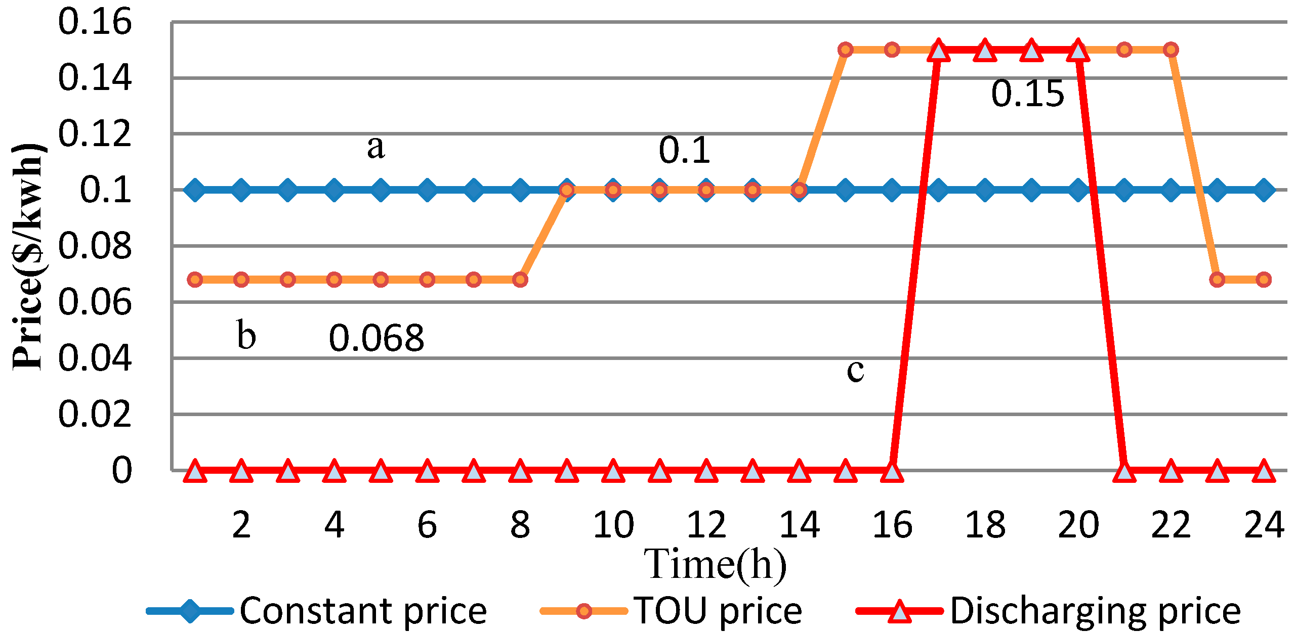
To analyze the charging and discharging behaviors of EVs under different price incentives, four cases are enumerated and investigated. The consumer-price elasticity matrix is referring to [34]. The price profiles of charging or discharging in different time are shown in Figure 4.

Case 1:

There are no EVs in the distribution network. As the uncertainty of regular load, the basic load at each bus follows a normal distribution, and the standard deviation is 10% of the mean values.

Case 2:

There are a total of 1000 EVs charging in five EV-stations with a daily constant price which is shown in Figure 4 (profile a). The basic load is same to that in Case 1.

Case 3:

There are 1000 EVs charging in five EV-stations with the TOU price, and the price profile of charging in this case is shown in Figure 4 (profile b). The basic load is same to that in Case 1.

Case 4:

There are totally 1000 EVs charging or discharging in five EV-stations. The TOU price of charging is same as Case 3. The discharging price is shown in Figure 4 (profile c). The basic load is same to that in Case 1.

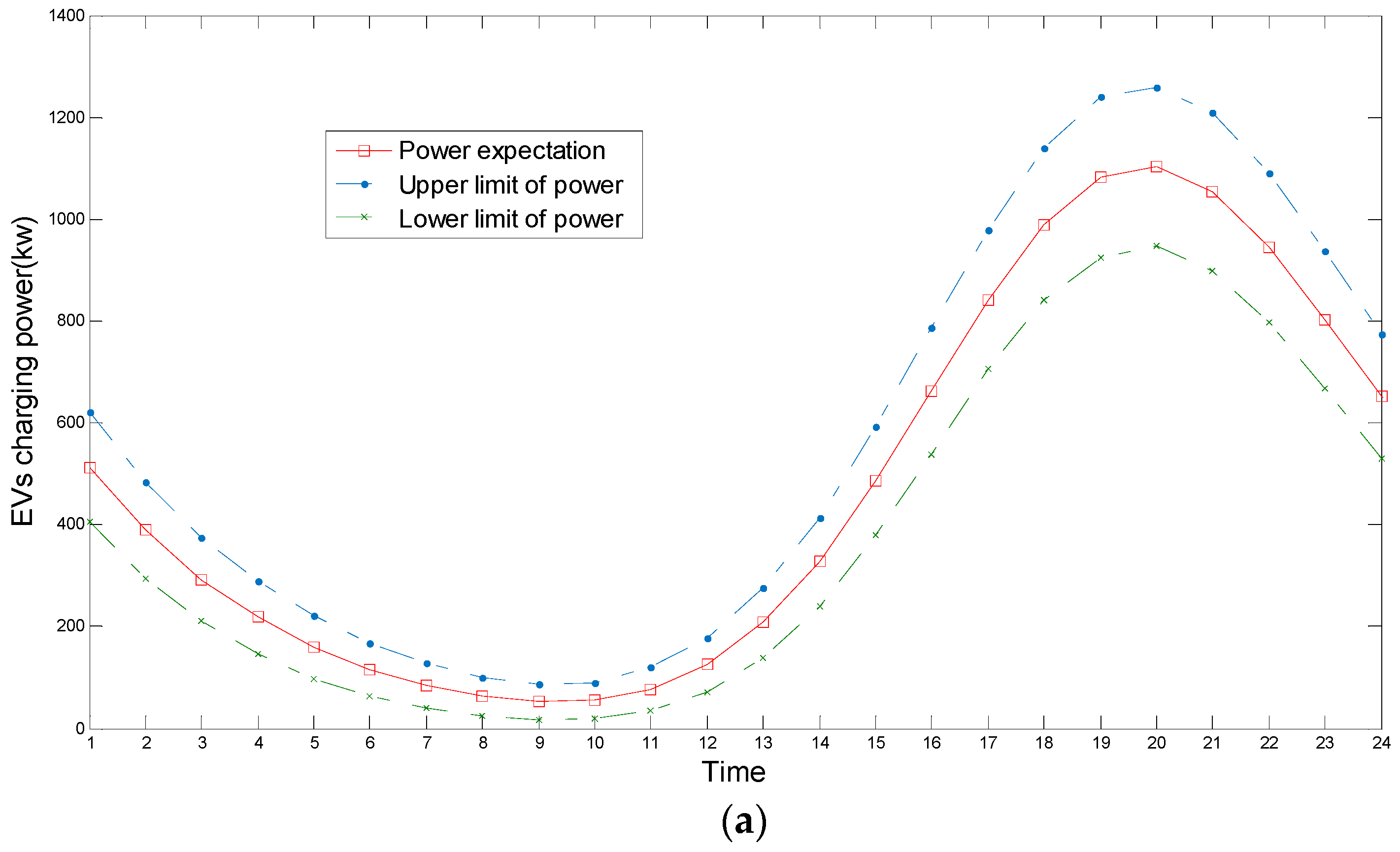
5.1. The Charging or Discharging Load of EVs under Different Electricity Prices

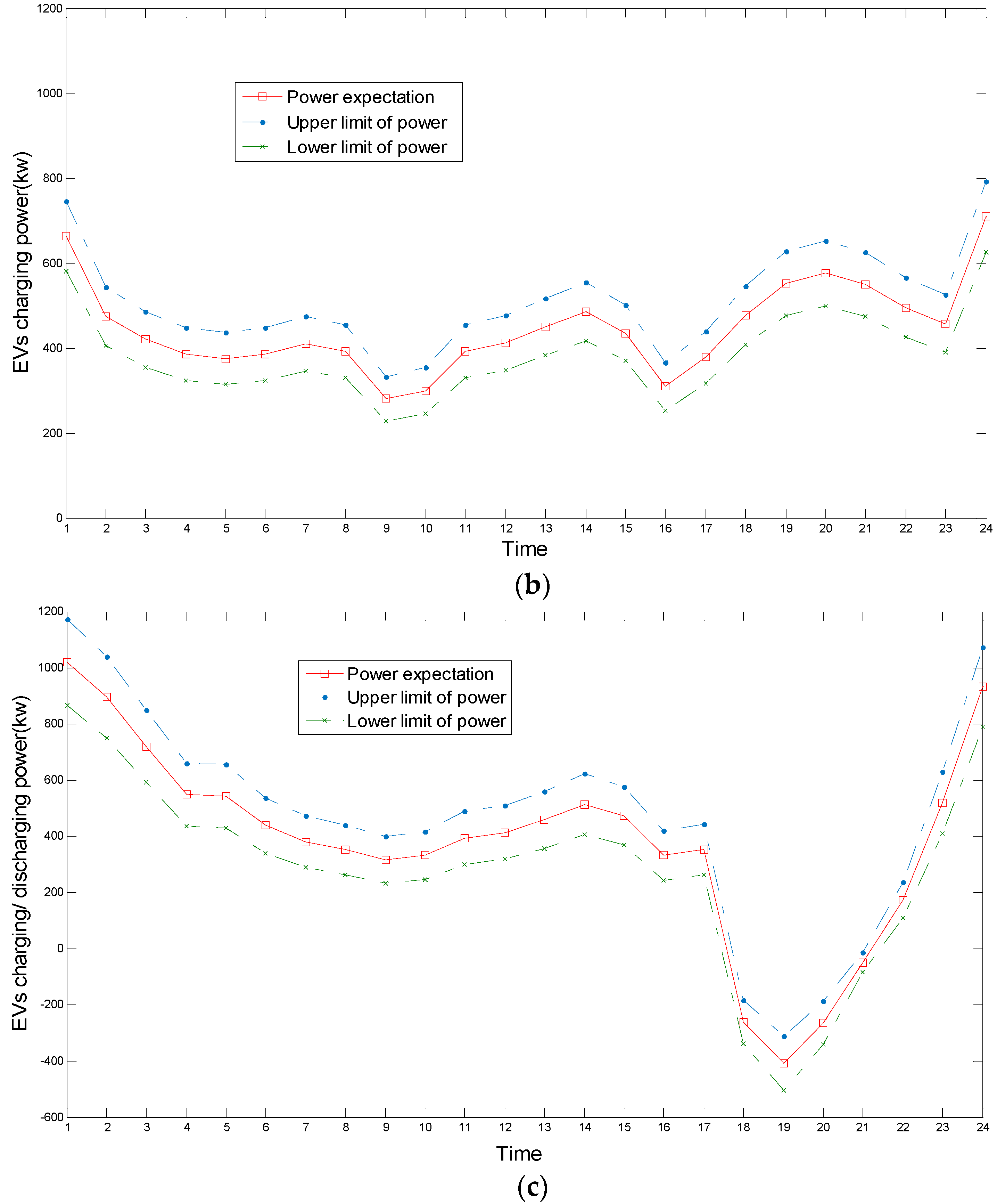
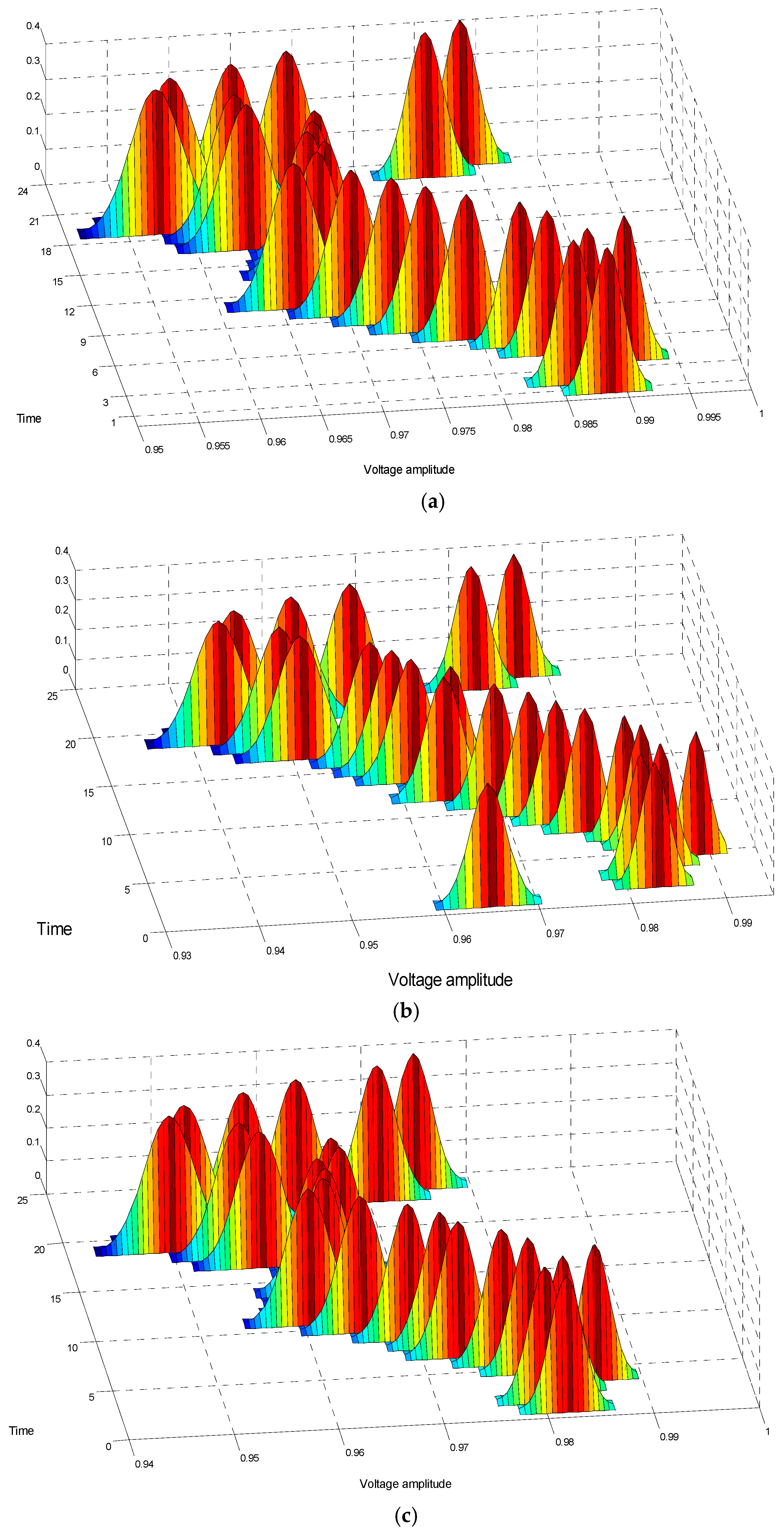
During the simulations, the battery capacity of each EV is supposed to be 15 kW·h for a cruise duration of 100 km, and the charging power P_c and discharging power P_d are both 2.5 kW [5]. Figure 5 shows the probability distribution of charging or discharging load of 1000 EVs within 24 h in case 2–4 calculated by MCS. As shown in Figure 5a, the peak load of the EVs charging occurs between 17:00 p.m. and 21:00 p.m. in Case 2, which is similar to the basic peak load. In Figure 5b, the ordinary TOU price is taken into account, and some EV users are guided to charge in off-peak time. It is found that the fluctuation of charging load decreases compared with Case 2. As shown in Figure 5c, when the discharging price at peak load is applied in Case 4, some EV users are guided to discharge in the peak hours and charge in valley period because of economic benefits.

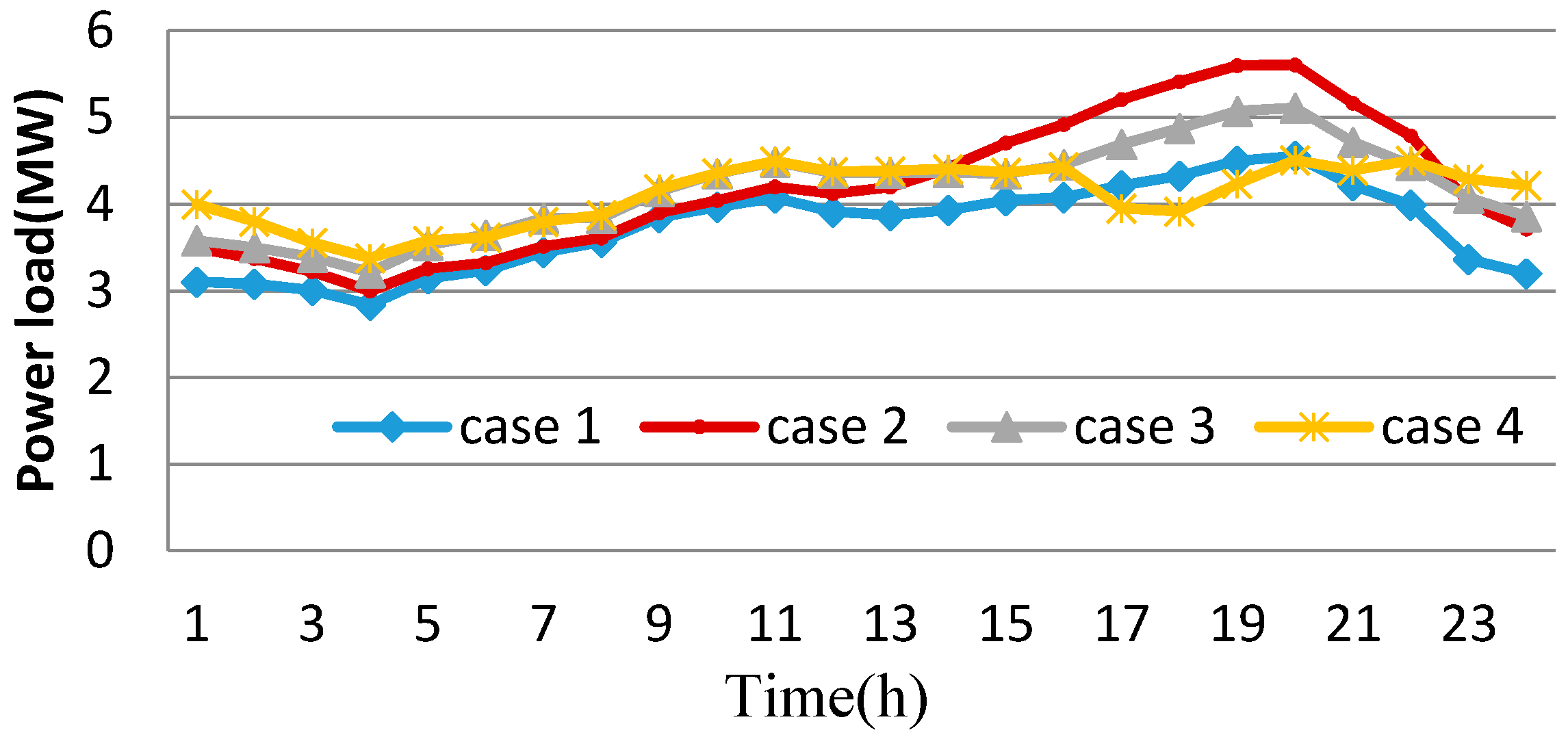
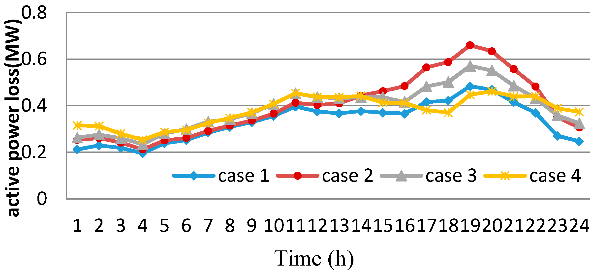
Figure 6 shows the load curves of the distribution network with different prices, and Figure 7 shows the active power loss curves. The difference in the peak-valley and the increase of the active power losses can be observed in Case 2, and it is because of the overlap between the basic peak load and the unordered EV charging power. Under the incentive of the TOU price in Case 3, the peak load and the power loss are both smaller than that in Case 2, but the peak-valley difference is greater than that in Case 1. When the improved TOU price is applied in Case 4, the peak-valley difference and the network power losses decrease significantly compared to the ordinary TOU price.

5.2. Risk Assessment of IEEE 33-Bus Distribution Network with EVs under Different Electricity Prices

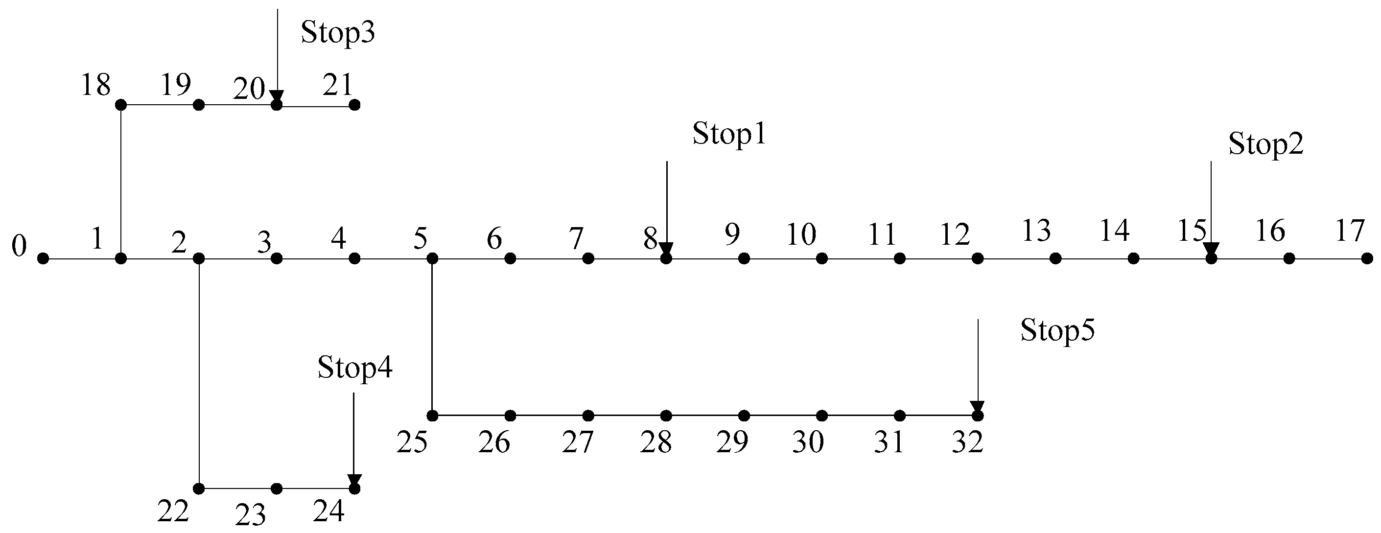
The schematic diagram of an IEEE 33-bus distribution network is shown in Figure 8. Stop 1–Stop 5 represent five EV-stations in the system, and the number of EVs in each station is shown in

Table 1. The number of EVs in each EV-station.

EV-Station	Stop 1	Stop 2	Stop 3	Stop 4	Stop 5
Node	8	15	20	24	32
Number	200	100	200	200	300

.

(1)

The risk assessment of node voltage in a day

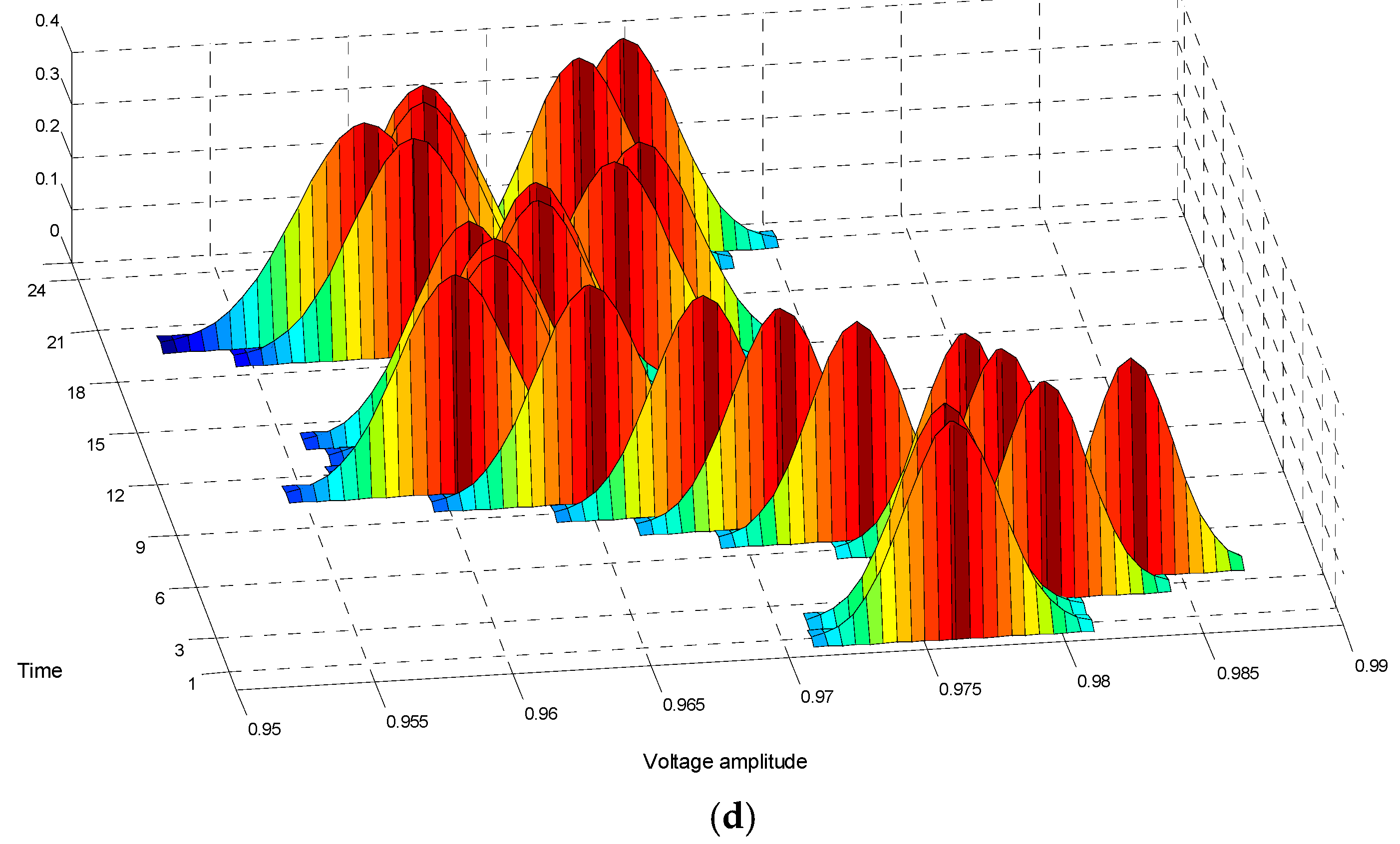
The probability distribution of voltage will fluctuate with the EV charging or discharging power and basic load, so that the node voltage may exceed the acceptable limit. As the bus 17 is located in the end of the distribution network, its node voltage is generally the lowest. Figure 9 shows the voltage distribution of the bus 17 under different cases. For Case 1, the voltage distribution of the bus 17 is maintained at an acceptable range. For Case 2, the voltage distribution of the bus 17 will be below the lower limit, especially when the system is justly in the peak load period (18:00 p.m.–21:00 p.m.). In addition, the fluctuation of the node voltage increases with the decrease of the expected value of the node voltage. Regarding that Case 3 is applied, the voltage being out of limits can be alleviated in contrast to Case 2, and it still exists in 18:00 p.m.–21:00 p.m. In Case 4, the voltage of the bus 17 is maintained at a reasonable level because of the voltage support caused by the discharging price of EVs.

Due to that the voltage distribution of the bus 17 in Case 1 and Case 4 can meet the requirements, the risks can be ignored in the system.

Table 2. The risk assessment results of the bus 17.

Case 2			Case 3
Time (h)	Off-Limit Probability	Risk Index (kW)	Time (h)	Off-Limit Probability	Risk Index (kW)
16	8.47 × 10−5	2.63 × 10−5	/	/	/
17	0.3434	0.912609	17	0.000121	4.59 × 10−5
18	0.6417	2.134106	18	0.0024	2.23 × 10−3
19	0.9965	5.621712	19	0.5288	1.68114
20	0.9745	4.829508	20	0.2475	0.64845
21	0.2528	0.620154	21	0.000221	1.03 × 10−4
22	5.76 × 10−5	1.43 × 10−5	/	/	/

shows the risk assessment results of the bus 17 in Case 2 and Case 3. The risk index of node voltage in Case 3 is much smaller than that in Case 2 at the same time. The results demonstrate that the reasonable electricity pricing mechanism of EVs can keep the node voltage in the acceptable range and reduce the operational risk of the distribution network.

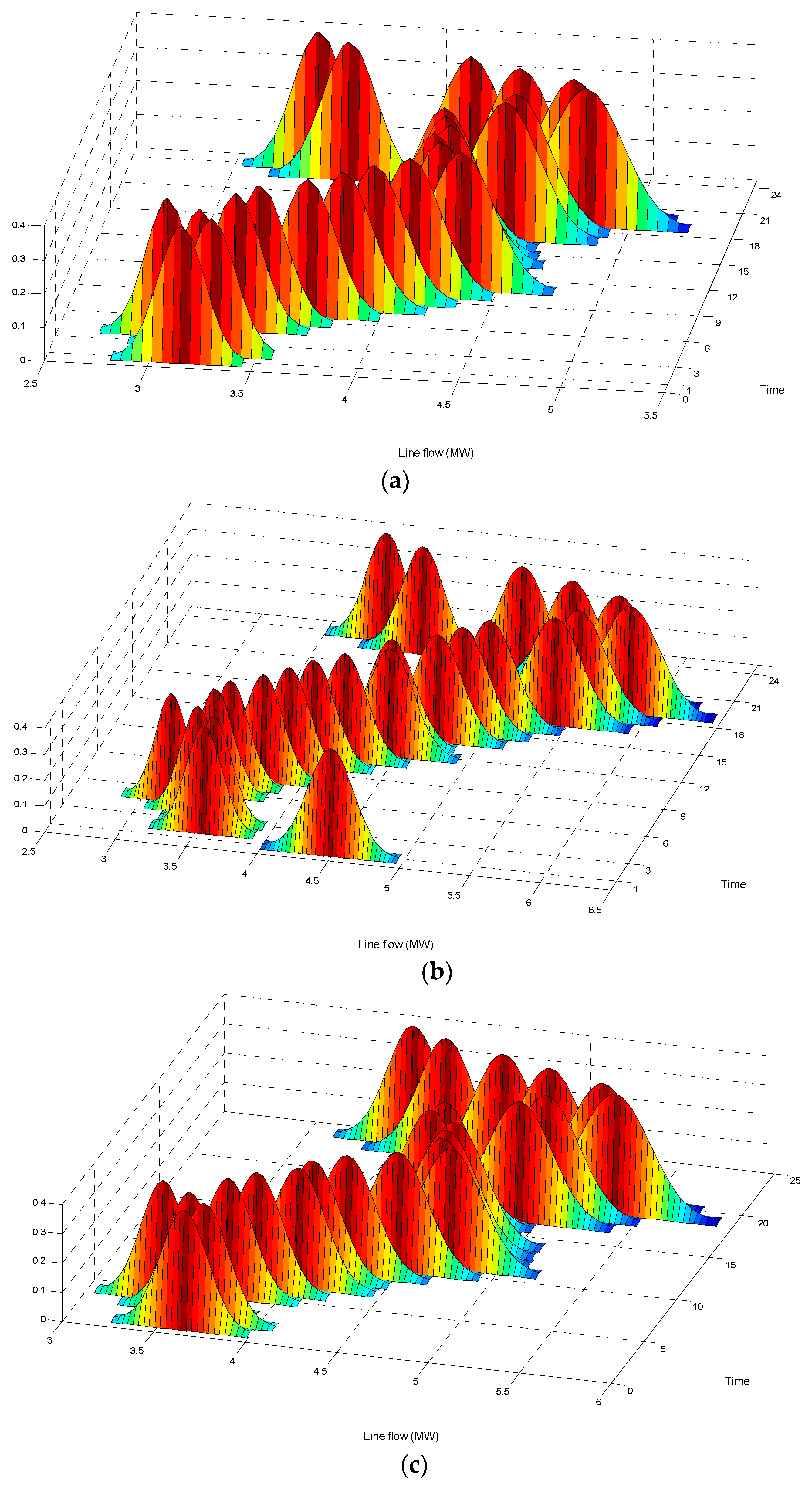
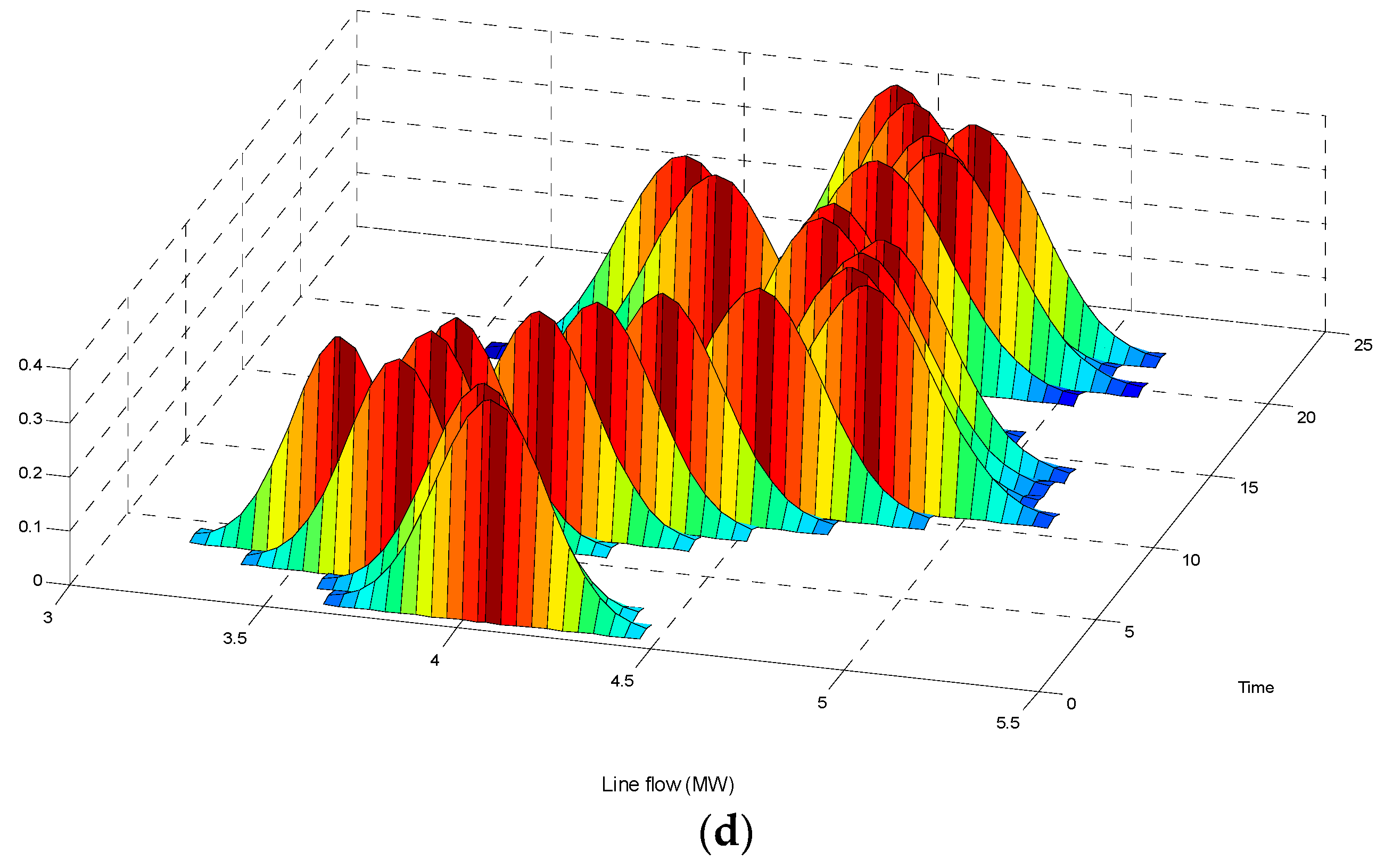
For that branch 0–1 belongs to the beginning end of the 33-bus distribution network, the maximum line flow can be obtained. Figure 10 shows the probabilistic distribution of line flow in branch 0–1 under different cases. In Case 1 and Case 4, the line flow distribution will be under the transmission power limit, and the risks are ignored.

Table 3. Risk assessment results of branch 0–1.

Case 2			Case 3
Time (h)	Off-Limit Probability	Risk Index (kW)	Time (h)	Off-Limit Probability	Risk Index (kW)
17	0.0349	106.9331	/	/	/
18	0.134	556.7524	18	0.0024	0.29366
19	0.7119	3984.643	19	0.0193	52.6212
20	0.4824	2704.036	20	0.0041	8.03353
21	0.0205	55.52134	/	/	/

shows the risk assessment results of branch 0–1 in Case 2 and Case 3.

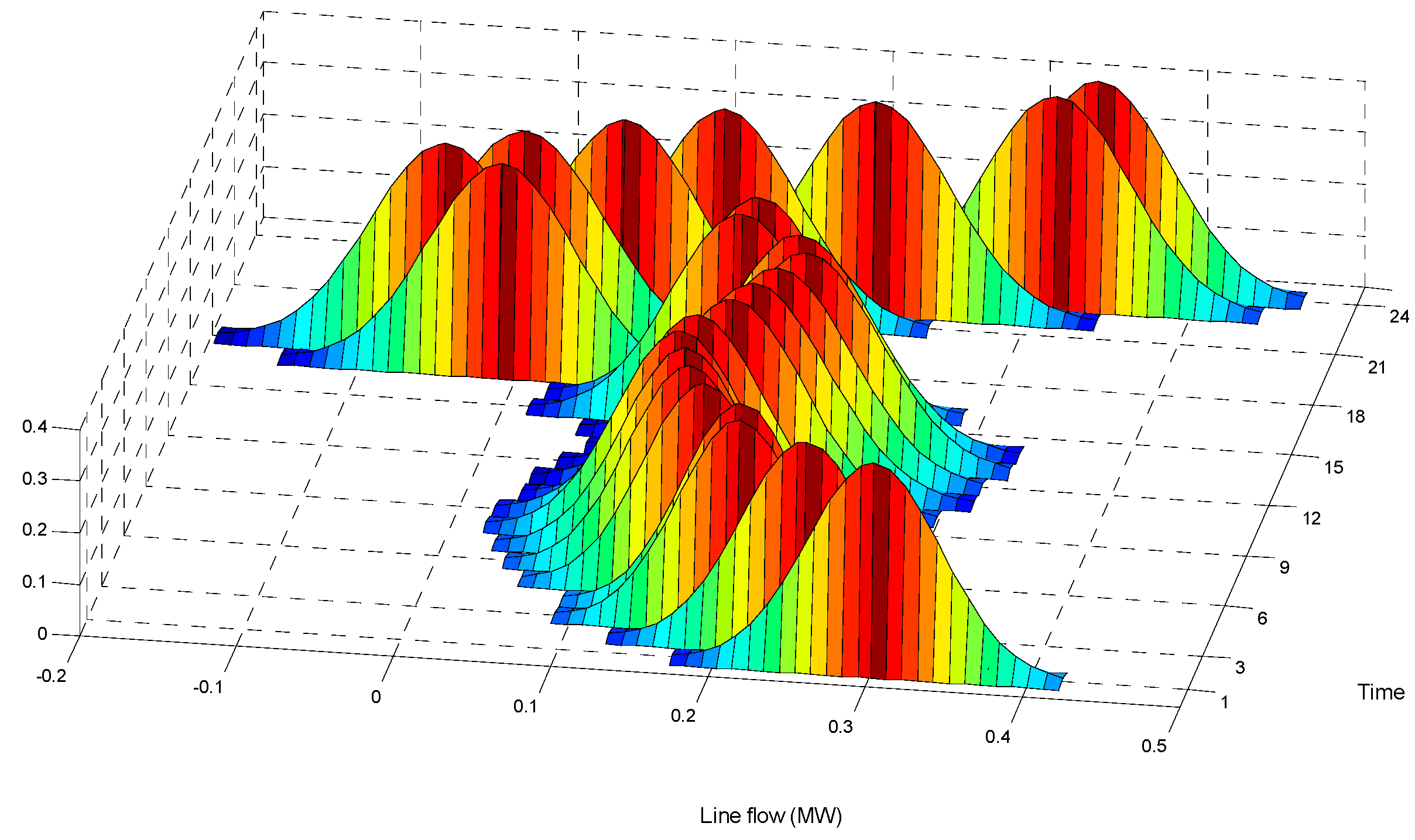
For Case 1, the line flow in branch 0–1 is smaller than the transmission power limit. For Case 2, the line flow exceeds the upper limit in the evening peak load period. In addition, the fluctuation of the power flow increases with the rise of the expected value of the power flow. For Case 3, the line flow being out of limits can be mitigated compared with Case 2. For Case 4, the line flow is well controlled with the improved TOU price, and according to Figure 11 where the flow in branch 31–32 is studies, the flow direction will reverse due to the discharging behavior of EVs in peak time.

(2)

The risk assessment of node voltage at 19:00 p.m.

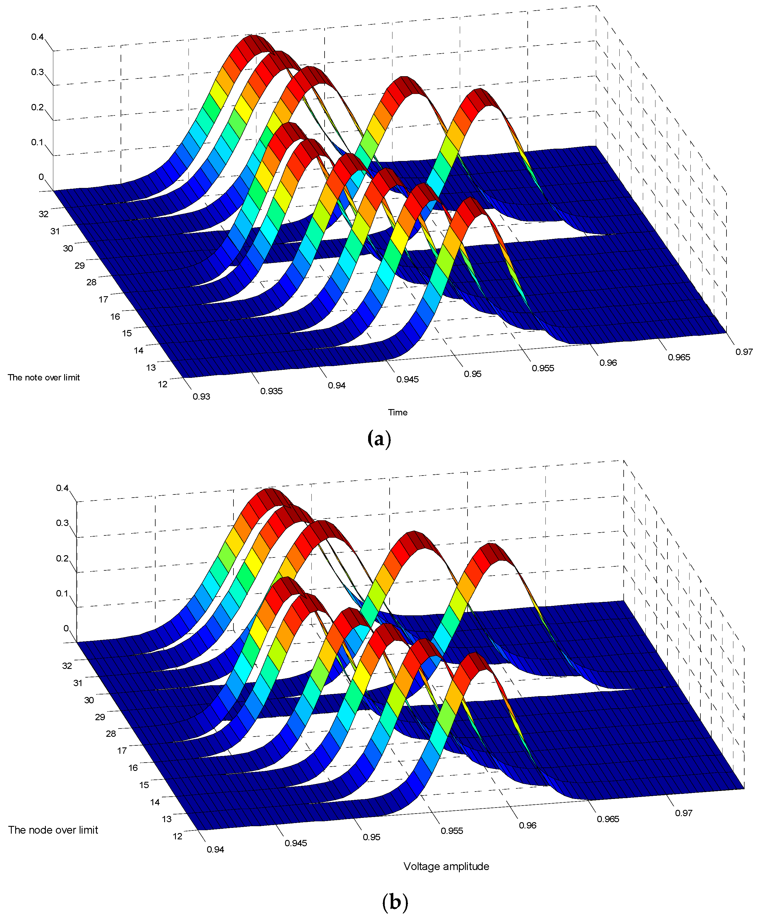
Based on the aforementioned simulation results, the node voltage being out of limits will be the most obvious at 19:00 p.m. In Case 1 and Case 4, all of the node voltages at 19:00 p.m. will not exceed the limit, and the safe operation of the network is ensured. For Case 2 and Case 3, Figure 12 shows the dangerous nodes whose voltages are smaller than the lower limit at 19:00 p.m., and the related off-limit probability and risk index are shown in

Table 4. Risk assessment results of distribution network at 19:00 p.m.

Case 2			Case 3
Node	Off-Limit Probability	Risk Index (kW)	Node	Off-Limit Probability	Risk Index (kW)
12	0.1911	1.71371	12	3.12 × 10−5	1.74 × 10−5
13	0.6113	15.41382	13	0.0036	0.025439
14	0.8445	12.60708	14	0.0297	0.163057
15	0.957	42.05221	15	0.1324	1.76685
16	0.9935	20.0628	16	0.4236	4.204446
17	0.9965	31.45754	17	0.5288	8.487008
28	0.0017	0.013999	/	/	/
29	0.1337	4.711244	29	2.72 × 10−4	0.002066
30	0.8217	38.53576	30	0.0757	1.618413
31	0.9165	66.60967	31	0.1617	5.726648
32	0.9508	116.3876	32	0.2209	8.052128

. It is found that, the voltage over the end-terminal node is prone to exceed the limitation in the radial distribution network. Comparing to the node voltage with the ordinary TOU price, the node voltage with the constant price is more likely to exceed the limit. For a certain node, the risk index of the node voltage in Case 3 is much smaller than that in Case 2.

5.3. Risk Assessment of IEEE 69-Bus Distribution Network with EVs under Different Electricity Prices

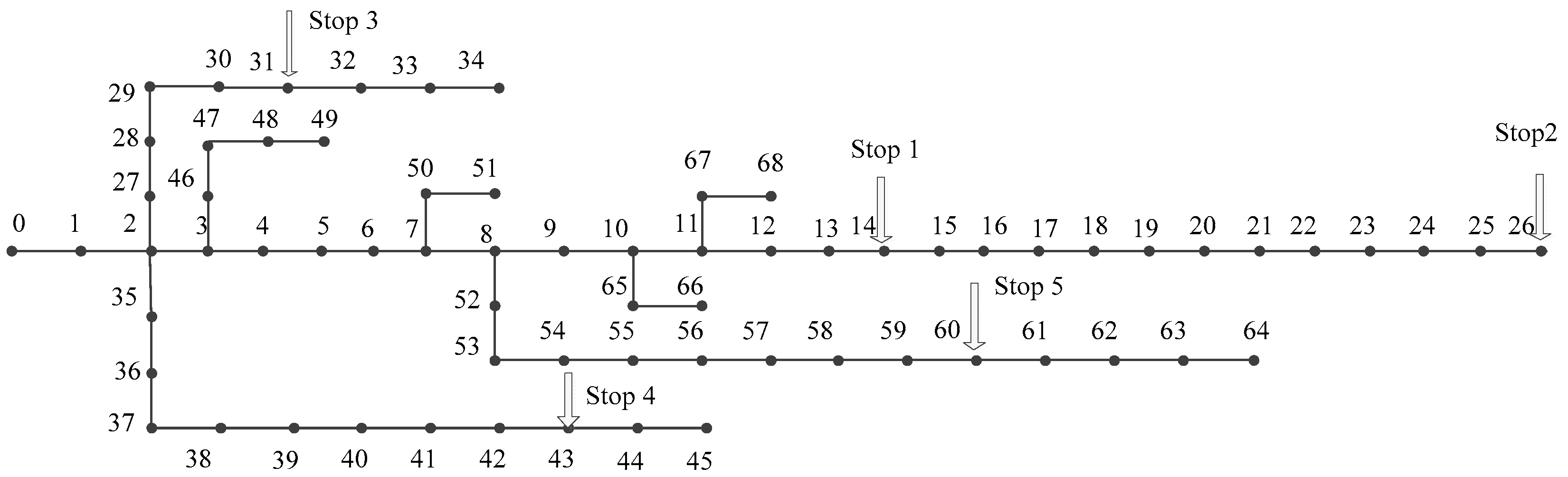
As shown in Figure 13, an IEEE 69-bus distribution network is further introduced to verify the method applicability. The number of EVs in each station is shown in

Table 5. The number of EVs in each EV-station.

EV-Station	Stop 1	Stop 2	Stop 3	Stop 4	Stop 5
Node	14	24	31	43	60
Number	200	300	100	200	200

.

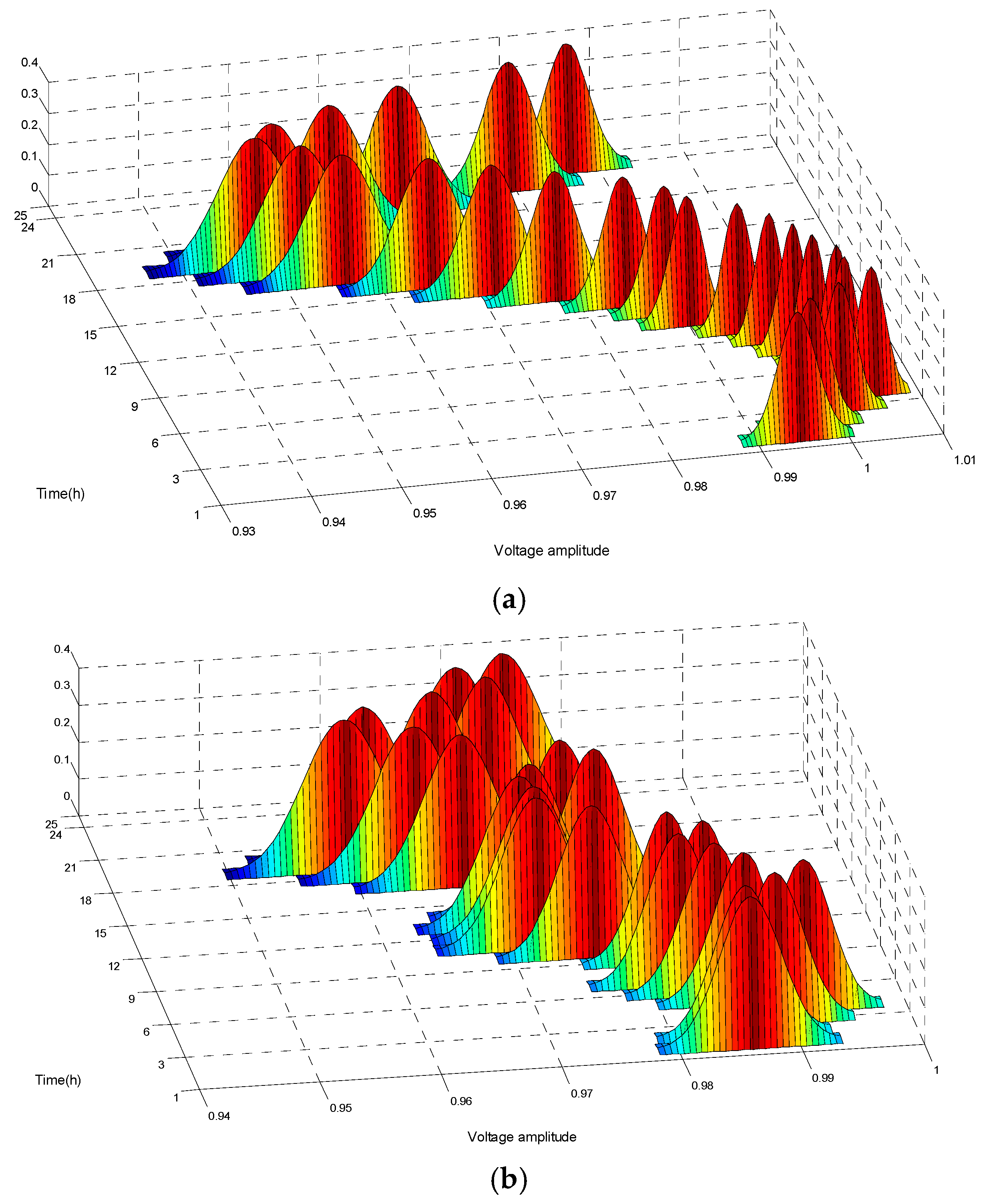
The voltage distribution of the terminal bus 26 is shown in Figure 14. For Case 1 and Case 4, all of the node voltages can be maintained in an acceptable range.

For Case 2 and Case 3,

Table 6. The risk assessment results of bus 26.

Case 2			Case 3
Time (h)	Off-Limit Probability	Risk Index (kW)	Time (h)	Off-Limit Probability	Risk Index (kW)
17	0.0398	0.322845	/	/	/
18	0.2564	3.460025	/	/	/
19	0.6751	12.48483	19	0.0018	4.23 × 10−5
20	0.41	6.01849	20	1.64 × 10−4	1.85 × 10−6
21	0.0119	0.071663	/	/	/

and

Table 7. Risk assessment results of branch 0–1.

Case 2			Case 3
Time (h)	Off-Limit Probability	Risk Index (kW)	Time (h)	Off-Limit Probability	Risk Index (kW)
17	0.0059	16.80197	/	/	/
18	0.0239	93.79097	/	/	/
19	0.2782	1586.746	19	0.0052	1.829538
20	0.1419	810.6977	20	0.0013	0.252245
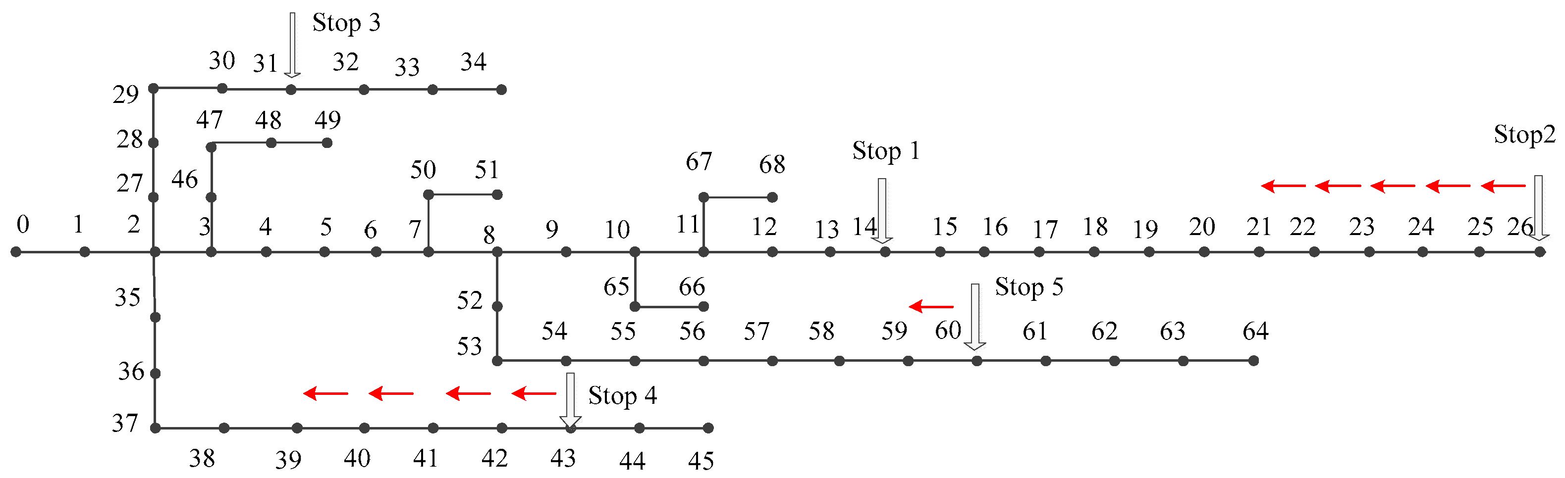
21	0.0036	9.285573	/	/	/

respectively indicate the risk assessment results of the bus 26 and branch 0–1. Meanwhile, considering the discharging behavior of EVs in Case 4, Figure 15 shows that the power flow in some branches will reverse.

The aforementioned simulations show that the IEEE 69-bus distribution network could obtain the consistent results with the IEEE 33-bus distribution network, and the availability and suitability of the proposed method can be confirmed.

6. Conclusions

Concerning that a large number of EVs can be connected to the distribution network for charging or discharging, it is critical to ensure safe and stable operation. This paper proposes a risk assessment method to evaluate the operational risk of the distribution network, and herein EVs’ charging/discharging behaviors and reasonable price incentive are taken into account. In terms of the constant price, ordinary TOU and an improved TOU price, three charging/discharging power models are constructed. A cumulants and Gram-Charlier series-based PLF calculation method is applied to calculate the power flow. The risk indexes of node voltage and line flow are given to analyze the safety risks. From the simulations of an IEEE-33 bus system and an IEEE 69-bus system, the availability and suitability of the proposed method are confirmed, and some conclusions are summarized as follows:

(1)

In view of the charging and discharging behaviors of EVs, the voltage over the end-terminal node of the distribution network is more likely to exceed the acceptable range, and the line flow in the beginning of the branch is easy to exceed the transmission power limit.

(2)

Different price mechanisms will affect the safety risks of the distribution network. When the uncoordinated charging with constant price is used, higher peak-valley difference, larger power losses and increase of the safety risks will be achieved.

(3)

Compared to the ordinary TOU price, using the improved TOU price can contribute to show better preference on reducing the peak-valley difference, and the safety of the distribution network can be enhanced.

(4)

The change of the distribution network’s structure will not affect the proposed method’s effectiveness, and the IEEE 69-bus distribution network could obtain the consistent results with the IEEE 33-bus distribution network.

In the near future, the optimal strategy for charging/discharging price of EVs will be performed, and the results will be reported in later articles.

References

1. Khodayar, M.E.; Wu, L.; Li, Z. Electric vehicle mobility in transmission-constrained hourly power generation scheduling. IEEE Trans. Smart Grid 2013, 4, 779–788. [Google Scholar] [CrossRef]
2. Fernandes, C.; Frías, P.; Latorre, J.M. Impact of vehicle-to-grid on power system operation costs: The Spanish case study. Appl. Energy 2012, 96, 194–202. [Google Scholar] [CrossRef]
3. Foley, A.; Tyther, B.; Calnan, P.; Gallachóir, B.Ó. Impacts of Electric Vehicle charging under electricity market operations. Appl. Energy 2013, 101, 93–102. [Google Scholar] [CrossRef]
4. Li, G.; Zhang, X.P. Modeling of plug-in hybrid electric vehicle charging demand in probabilistic power flow calculations. IEEE Trans. Smart Grid 2012, 3, 492–499. [Google Scholar] [CrossRef]
5. Tian, L.; Shi, S.; Jia, Z. A Statistical Model for Charging Power Demand of Electric Vehicles. J. Power Syst. Technol. 2010, 11, 126–130. [Google Scholar]
6. Wang, H.; Song, Q.; Zhang, L.; Wen, F.; Huang, J. Load characteristics of electric vehicles in charging and discharging states and impacts on distribution systems. In Proceedings of the International Conference on Sustainable Power Generation and Supply, Hangzhou, China, 8–9 September 2012; pp. 3616–3620.
7. Gao, T.; Liu, R.; Hua, K. Dispatching strategy optimization for orderly charging and discharging of electric vehicle battery charging and swapping station. In Proceedings of the 5th International Conference on Electric Utility Deregulation and Restructuring and Power Technologies (DRPT), Changsha, China, 26–29 November 2015; pp. 2640–2645.
8. Schneider, K.; Gerkensmeyer, C.; Kintner-Meyer, M.; Fletcher, M. Impact assessment of plug-in hybrid electric vehicles on pacific north-west distribution systems. In Proceedings of the 2008 IEEE Power and Energy Society General Meeting—Conversion and Delivery of Electrical Energy in the 21st Century, Pittsburgh, PA, USA, 20–24 July 2008; pp. 1–6.
9. Clement-Nyns, K.; Haesen, E.; Driesen, J. The impact of charging plug-in hybrid electric vehicles on a residential distribution grid. IEEE Trans. Power Syst. 2010, 25, 371–380. [Google Scholar] [CrossRef] [Green Version]
10. Salah, F.; Ilg, J.P.; Flath, C.M.; Basse, H.; van Dinther, C. Impact of electric vehicles on distribution substations: A Swiss case study. Appl. Energy 2015, 137, 88–96. [Google Scholar] [CrossRef]
11. Green, R.C.; Wang, L.; Alam, M. The impact of plug-in hybrid electric vehicles on distribution networks: A review and outlook. Renew. Sustain. Energy Rev. 2011, 15, 544–553. [Google Scholar] [CrossRef]
12. Huang, Y.; Guo, C.; Ding, Y.; Wang, L.; Zhu, B.; Xu, L. A Multi-Period Framework for Coordinated Dispatch of Plug-in Electric Vehicles. Energies 2016, 9, 370. [Google Scholar] [CrossRef]
13. Yang, Z.; Li, K.; Foley, A. Computational scheduling methods for integrating plug-in electric vehicles with power systems: A review. Renew. Sustain. Energy Rev. 2015, 51, 396–416. [Google Scholar] [CrossRef]
14. Lassila, J.; Haakana, J.; Tikka, V.; Partanen, J. Methodology to analyze the economic effects of electric cars as energy storages. IEEE Trans. Smart Grid 2012, 3, 506–516. [Google Scholar] [CrossRef]
15. Gao, Y.J.; Lü, M.; Wang, Q.; Liang, H.; Zhang, J. Research on Optimal TOU Price Considering Electric Vehicles Charging and Discharging Based on Discrete Attractive. J. Model Proc. CSEE 2014, 34, 3647–3653. [Google Scholar]
16. Chen, L.; Chen, Z.; Huang, X.; Jin, L. A Study on Price-Based Charging Strategy for Electric Vehicles on Expressways. Energies 2016, 9, 385. [Google Scholar] [CrossRef]
17. Cao, Y.; Tang, S.; Li, C.; Zhang, P.; Tan, Y.; Zhang, Z.; Li, J. An optimized EV charging model considering TOU price and SOC curve. IEEE Trans. Smart Grid 2012, 3, 388–393. [Google Scholar] [CrossRef]
18. Yang, H.; Yang, S.; Xu, Y.; Cao, E.; Lai, M.; Dong, Z. Electric Vehicle Route Optimization Considering Time-of-Use Electricity Price by Learnable Partheno-Genetic Algorithm. IEEE Trans. Smart Grid 2015, 6, 657–666. [Google Scholar] [CrossRef]
19. Dubey, A.; Santoso, S.; Cloud, M.P.; Waclawiak, M. Determining Time-of-Use Schedules for Electric Vehicle Loads: A Practical Perspective. IEEE Power Energy Technol. Syst. J. 2015, 2, 12–20. [Google Scholar] [CrossRef]
20. He, Y.; Venkatesh, B.; Guan, L. Optimal scheduling for charging and discharging of electric vehicles. IEEE Trans. Smart Grid 2012, 3, 1095–1105. [Google Scholar] [CrossRef]
21. Quinn, C.; Zimmerly, D.; Bradley, T. The effect of communication architecture on the availability, reliability, and economics of plug-in hybrid electric vehicle-to-grid ancillary services. J. Power Sources 2010, 195, 1500–1509. [Google Scholar] [CrossRef]
22. Gao, Y.; Wang, C.; Wang, Z.; Liang, H. Research on time-of-use price applying to electric vehicles charging. In Proceedings of the Innovative Smart Grid Technologies—Asia, Tianjin, China, 21–24 May 2012; pp. 1–6.
23. Zhang, P.; Lee, S.T. Probabilistic load flow computation using the method of combined cumulants and Gram-Charlier expansion. IEEE Trans. Power Syst. 2004, 19, 676–682. [Google Scholar] [CrossRef]
24. Dong, L.; Cheng, W.; Bao, H.; Yang, Y. Probabilistic load flow analysis for power system containing wind farms. In Proceedings of the 2010 Asia-Pacific Power and Energy Engineering Conference (APPEEC), Chengdu, China, 28–31 March 2010; pp. 1–4.
25. Negnevitsky, M.; Nguyen, D.H.; Piekutowski, M. Risk assessment for power system operation planning with high wind power penetration. IEEE Trans. Power Syst. 2015, 30, 1359–1368. [Google Scholar] [CrossRef]
26. Feng, Y.; Wu, W.; Zhang, B.; Li, W. Power system operation risk assessment using credibility theory. IEEE Trans. Power Syst. 2008, 23, 1309–1318. [Google Scholar] [CrossRef]
27. Deng, W.; Ding, H.; Zhang, B.; Lin, X.; Bie, H.; Wu, J. Multi-period probabilistic-scenario risk assessment of power system in wind power uncertain environment. IET Gener. Transm. Distrib. 2016, 10, 359–365. [Google Scholar] [CrossRef]
28. Hu, H. Distribution Network Risk Assessment Research Considering the Impact of Wind Power and Electric Vehicle; Huazhong University of Science & Technology: Wuhan, China, 2012. [Google Scholar]
29. Taylor, M.J.; Alexander, A. Evaluation of the impact of plug-in electric vehicle loading on distribution system operations. In Proceedings of the IEEE Power & Energy Society General Meeting, Calgary, AB, Canada, 26–30 July 2009; pp. 1–6.
30. Xiang, D.; Song, Y.; Hu, Z.C. Research on Optimal Time of Use Price for Electric Vehicle Participating V2G. Proc. CSEE 2013, 33, 15–25. [Google Scholar]
31. Liu, P.; Wu, G. Analysis of two typical voltage collapse accidents in the world. J. Int. Power 2003, 5, 35–37. [Google Scholar]
32. Baran, M.E.; Wu, F.F. Network reconfiguration in distribution systems for loss reduction and load balancing. IEEE Trans. Power Deliv. 1989, 4, 1401–1407. [Google Scholar] [CrossRef]
33. Baran, M.E.; Wu, F.F. Optimal capacitor placement on radial distribution systems. IEEE Trans. Power Deliv. 1989, 4, 725–734. [Google Scholar] [CrossRef]
34. Lv, M.K. Research on TOU Price Considering Electric Vehicles Charging and Discharging; North China Electric Power University: Beijing, China, 2014. [Google Scholar]
Figure 1. The flowchart of PLF based on cumulants and Gram-Charlier series.
Energies 09 00560 g001
Figure 2. (a) Mathematical relationship between the load losses and the voltage over upper limit; (b) Mathematical relationship between the load losses and the voltage below lower limit.
Energies 09 00560 g002
Figure 3. Mathematical relationship between the line flow off-limit and the load losses.
Energies 09 00560 g003
Figure 4. Three different electricity price profiles.
Energies 09 00560 g004
Figure 5. The charging/ discharging load profiles of 1000 EVs. (a) Case 2; (b) Case 3; (c) Case 4.
Energies 09 00560 g005aEnergies 09 00560 g005b
Figure 6. Load curves of distribution network in different cases.
Energies 09 00560 g006
Figure 7. Active power loss curves of power distribution network in different cases.
Energies 09 00560 g007
Figure 8. An IEEE 33-bus distribution network.
Energies 09 00560 g008
Figure 9. The voltage probabilistic distribution of the bus 17 under different cases. (a) Case 1; (b) Case 2; (c) Case 3; (d) Case 4.
Energies 09 00560 g009aEnergies 09 00560 g009b
Figure 10. Line flow probabilistic distribution of branch 0–1. (a) Case 1; (b) Case 2; (c) Case 3; (d) Case 4.
Energies 09 00560 g010aEnergies 09 00560 g010b
Figure 11. Line flow probabilistic distribution of branch 31–32 in Case 4.
Energies 09 00560 g011
Figure 12. The node over limit at 19:00 p.m. (a) Case 2; (b) Case 3.
Energies 09 00560 g012
Figure 13. An IEEE 69-bus distribution network.
Energies 09 00560 g013
Figure 14. The voltage probabilistic distribution of bus 26. (a) Case 2; (b) Case 3.
Energies 09 00560 g014
Figure 15. The reverse flow of case 4 at 18:00 p.m.
Energies 09 00560 g015