Indirect Load Control for Energy Storage Systems Using Incentive Pricing under Time-of-Use Tariff

Abstract

Indirect load control (ILC) is a method by which the customer determines load reduction of electricity by using a price signal. One of the ILCs is a time-of-use (TOU) tariff, which is the most commonly used time-varying retail pricing. Under the TOU tariff, the customer can reduce the energy cost through an energy storage system (ESS). However, because this tariff is fixed for several months, the ESS operation does not truly reflect the wholesale market price, which could widely fluctuate. To overcome this limitation, this paper proposes an incentive pricing method in which the load-serving entity (LSE) gives the incentive pricing signal to the customers with ESSs. Because the ESS charging schedule is determined by the customer through ILC, a bilevel optimization problem that includes the customer optimization problem is utilized to determine the incentive pricing signal. Further, the bilevel optimization problem is reformulated into a one-level problem to be solved by an interior point method. In the proposed incentive scheme: (1) the social welfare increases and (2) the increased social welfare can be equitably divided between the LSE and the customer; and (3) the proposed incentive scheme leads the customer to voluntarily follow the pricing signal.

1. Introduction

Traditionally, in order to maintain the balance between electricity demand and supply, it was inevitable to install new infrastructure, such as generators, transmission lines, and distribution lines. However, such an approach may be constrained by space, finance, and the physical environment. In addition, for peak demand, the production cost is high, thus increasing the energy cost under this approach. Thus, demand-side management (DSM), which involves control of the demand for the various operations, is one of the alternatives to the expansion approach. Through DSM, utilities and load-serving entities (LSEs) can reduce their operating costs and defer the upgrade of their network and improve system reliabilities [1,2,3]. In addition, by participating in the DSM, the customers can reduce their electricity bills or make the incentives.

DSM can be categorized into direct load control and indirect load control (ILC) [4]. In direct load control, the LSE determines the amount of customer load reduction based on a predetermined contract. If the customer receives the command of load reduction, he/she has two choices: To make a profit when he/she follows the LSE decision, or to make use of electricity without inconvenience and with the possibility of penalty. On the other hand, in the ILC scheme, the customer determines the amount of load reduction based on information from the LSE. Price-based programs that adjust different prices depending on the system condition can be classified as the ILC. The price-based programs induce the customer to reduce consumption voluntarily by ensuring his/her profit [5].

Time-of-use (TOU) pricing and real-time pricing (RTP) can be seen as the two mainly considered price-based ILCs. TOU prices are divided into different fixed price blocks, namely, peak, mid-peak, and off-peak prices. Because TOU rates are adjusted for some duration, for example, a season, the TOU tariff can be seen as a stable tariff. Therefore, the TOU tariff can make the customer adapt to time-varying price more easily [4]. The RTP varies in response to the wholesale prices. Because the TOU pricing does not reflect the wholesale price immediately compared to RTP, the benefit from RTP is greater than that from TOU pricing [6]. However, RTP has several drawbacks. First, for the RTP, enabling technologies, such as those that communicate between the LSE and the customers and optimize the load profile, are required [7]. Second, because the RTP tariff transfers the uncertainty and volatility of wholesale prices to customers, it does not tend to attract many customers [8]. Thus, TOU is the most popular time-varying price tariff in the world [9].

Meanwhile, because an energy storage system (ESS) can respond to the price signal quickly, the ESS is suitable for the ILC. The method to design RTP for peak reduction of the total system demand is proposed in [10,11,12]. In [10], where the retail price is estimated based on the squared value of total load, when the customers try to reduce their cost, the peak-to-average ratio is also reduced. In [11], in order to maintain customer demand as a specified amount of energy, the price of energy increases in proportion to the deviation of the actual energy demand from the specified amount. When the customer can reduce his/her cost through the ESS, the total demand is maintained within certain ranges. In [12], by proposing the quadratic cost function and utilizing the game theory, the peak decreases. It is verified that the ESS reduces the energy cost in response to RTP in [13,14]. The ESS charging schedules are determined by linear programming to minimize the retail cost. Because the RTP reflects the wholesale market, the energy cost of the LSE reduces. The utilizations of ESS under TOU tariff are presented in [15,16]. The method to determine the optimal size of ESSs under TOU rates is proposed using dynamic programming [15]. In [16], which considers a wind turbine generator with particle swarm optimization, the method to determine the optimal ESS schedule for TOU rates is proposed. In [17], a two-stage optimization problem is proposed for increasing the profit of the customer who participates in the DSM using the ESS. In the first stage, the capacity of the ESS and the appropriate combination of the ILC are determined. In the second stage, the outputs of the ESS and the DG are determined based on the decisions in the first stage.

In summary, the ESS can be used for ILC based on both RTP and TOU because of fast response to pricing signal. Because the TOU pricing is fixed for several months, the wholesale market cost savings from the ESS in RTP is better compared to TOU pricing [14,18]. However, TOU pricing is the most commonly used retail pricing tariff because of the customer acceptability mentioned above. In this paper, the ILC that improves the reduction of the energy cost under the TOU tariff is proposed using the incentive pricing signal for the ESS operation. In order to overcome the limitation of the ESS utilization in the TOU rates, it is assumed that the additional measurement is implemented at the ESS owned by the customer. Then, the LSE determines the incentive pricing signal for ESS operation and sends the signal to customers. From the pricing signal and additional measurement, the total incentives of the customers are determined. Therefore, the customer can make two types of profits through the ESS: The cost savings in the TOU tariff and the incentive for the ESS operation. Simultaneously, the LSE can reduce the purchasing cost in the wholesale market because the incentive pricing signal changes the ESS charging schedules of the customers.

In order to determine the incentive pricing signal for the ESS operation, the LSE receives the information of the ESS from the owner and predicts the wholesale market price, for example, system marginal price (SMP). Because the ESS charging schedule is determined by the customer for maximizing his/her profit under the ILC, the total optimization problem of the LSE is formulated to a bilevel optimization problem, which includes the optimization problem of the customer. The upper-level problem (ULP) is related to the LSE profit and the lower-level problem (LLP) to the customer behavior for the incentive pricing signal. Through the bilevel optimization, the incentive pricing signal is determined. In order to verify the proposed incentive method, the profits of the customer and LSE in this method are compared with the profits of the customer and LSE under the TOU rates.

The main contributions are summarized as follows:

• In order to improve the ESS utilization in the TOU rates, the incentive price for the ESS operation is utilized and the effect of the incentive price is verified.
• Because the ESS charging schedule is determined by the customer under ILC, a bilevel optimization problem is introduced. Further, in order to attract customers to the incentive scheme and to divide the increased social welfare equitably, the method to determine proper incentive pricing is proposed.
• In order to solve the bilevel problem by using an interior point method, the procedure of reformulating the bilevel optimization is presented. The procedure is composed of reformulating the piecewise linear constraint to a linear constraint, adjusting the Karush–Kuhn–Tucker (KKT) conditions of the LLP, and using the penalty methods.

The rest of this paper is organized as follows. The detailed system model is presented in Section 2. The formulation of the bilevel optimization problem is presented in Section 3. Because it is difficult to solve the bilevel optimization problem by using an interior point method, the procedure of reformulating the bilevel optimization is presented in Section 4. The effect of the proposed incentive scheme is analyzed in Section 5. Finally, Section 6 concludes the paper.

2. System Model

Despite the fast response of the ESS, it is difficult for the ESS operation owned by the customer to reflect the variability of the wholesale market price under the TOU rates. In order to utilize the ESS more economically, an additional measurement is implemented at the ESS, as shown in Figure 1. The load demand including the ESS operation is measured by the load measurement and the ESS operation is measured by the ESS measurement independently. Further, the LSE gives the incentive pricing signal for the ESS operation to the customer. Under this system model, the incentive for the ESS operation is determined from the incentive price and the ESS operation. The customer can profit from the load reduction caused by the ESS operation based on the load measurement. Additionally, it is possible to reward for the ESS operation irrespective of the other load devices based on the ESS measurement. On the other hand, using the incentive pricing signal, the LSE can influence the charging schedule of the ESS owned by the customer more directly compared to that using only the TOU rates.

The overall process of determining the ESS charging schedule is illustrated in Figure 2. The incentive price scheme is the day-ahead DSM. The LSE receives the individual information of the ESS, that is, state of charge (SOC), maximum charging and discharging power, capacities, and charging and discharging efficiencies, from the customers and predicts the SMP. Then, the LSE determines the incentive pricing signal for the ESS operation based on SMP, TOU, and the ESS information and sends this signal to the customers. The detailed process of determining the pricing signal is presented in Section 3 and Section 4. Finally, the customers determine their ESS charging schedules by the TOU price and the incentive pricing signal. By this process, the customers can increase the benefit from the incentive and the LSE can reduce the cost from the wholesale market.

With the development of smart grid technologies, the communication technologies such as ZigBee, wireless mesh, cellular network communication, powerline communication, digital subscriber lines, and optical fiber, are utilized for communication between the LSE and the customers. The detailed information of the communication technologies is presented in [19,20]. Under the day-ahead DSM, high communication speed is not required and delay of the communication of the data can be tolerated. However, if the incentive price scheme is expanded into the real-time DSM, communication speed and delay should be considered.

3. Problem Formulation

Because the final ESS charging schedule is determined by the ESS customer under the ILC, the LSE should consider the customer behavior depending on the incentive pricing signal for the ESS operation. In other words, an optimization problem related to the profit of the customer should be embedded in the total optimization problem in which the LSE determines the incentive price. Therefore, the optimization problem of the LSE can be formulated as a bilevel optimization problem. A bilevel problem is the optimization problem where an optimization problem is embedded with another. The ULP is the outer optimization problem and the LLP is the inner optimization problem, which is included as a constraint of the ULP. The ULP maximizes the profit of the LSE. The LLP maximizes the profit of the customers and is the constraint of the ESS charging schedule in the total optimization problem.

3.1. Upper-Level Problem

The purpose of the ULP is to maximize the profit of the LSE. The profit of the LSE can be calculated by the revenue of the LSE and the cost of the LSE. Because the LSE sells the electricity with the TOU tariff, the revenue of the LSE from the customer with the ESS can be obtained as:

$${Revenue}_{\text{LSE}}={\displaystyle \sum _{t=1}^{N_{\mathrm{T}}}{C}_{\mathrm{R},t}\left({\displaystyle \sum _{i=1}^{N_{\mathrm{D}}}\left(P_{\mathrm{d},i,t}-P_{\text{ESS},i,t}\right)}\right)}$$

(1)

where C_R,t is the retail price in TOU tariff at time t; P_d,i,t is the load demand of customer i at time t; P_EES,i,t is the power output of ESS of customer i at time t; N_T is the number of time periods; and N_D is the number of customers with ESS.

The LSE buys the electricity with the SMP from the wholesale market. Further, in the proposed scheme, the LSE gives the incentive to the customers. Therefore, the cost of the LSE can be written as the sum of the purchase cost and the expenditure of the incentive:

$$Cos{t}_{\text{LSE}}={\displaystyle \sum _{t=1}^{N_{\mathrm{T}}}{C}_{\mathrm{S},t}\left({\displaystyle \sum _{i=1}^{N_{\mathrm{D}}}\left(P_{\mathrm{d},i,t}-P_{\text{ESS},i,t}\right)}\right)}+{\displaystyle \sum _{t=1}^{N_{\mathrm{T}}}{C}_{\mathrm{I},t}\left({\displaystyle \sum _{i=1}^{N_{\mathrm{D}}}{P}_{\text{ESS},i,t}}\right)}$$

(2)

where C_S,t is the SMP at time t and C_I,t is the incentive price at time t. The objective of the LSE is to maximize the profit. In other words, the objective function can be written as the minimization of the negative value of the profit:

$$\underset{C_{\mathrm{I},t},P_{\text{ESS},i,t}}{\min }\left({\displaystyle \sum _{t=1}^{N_{\mathrm{T}}}\left(C_{\mathrm{S},t}\left({\displaystyle \sum _{i=1}^{N_{\mathrm{D}}}\left(P_{\mathrm{d},i,t}-P_{\text{ESS},i,t}\right)}\right)+C_{\mathrm{I},t}\left({\displaystyle \sum _{i=1}^{N_{\mathrm{D}}}{P}_{\text{ESS},i,t}}\right)-C_{\mathrm{R},t}\left({\displaystyle \sum _{i=1}^{N_{\mathrm{D}}}\left(P_{\mathrm{d},i,t}-P_{\text{ESS},i,t}\right)}\right)\right)}\right)$$

(3)

The load demand changes depending on the retail price by the customer. The retail price in the TOU rates is the fixed value for several months. In addition, the SMP and the incentive pricing signal do not have an effect on the load demand. Therefore, the load demand is seen as a constant value in the proposed incentive scheme. Equation (3) can be simplified as:

$$\underset{C_{\mathrm{I},t},P_{\text{ESS},i,t}}{\min }\left({\displaystyle \sum _{t=1}^{N_T}\left(\left(-C_{\mathrm{S},t}+C_{\mathrm{I},t}+C_{\mathrm{R},t}\right)\left({\displaystyle \sum _{i=1}^{N_{\mathrm{D}}}{P}_{\text{ESS},i,t}}\right)\right)}\right)$$

(4)

In order to make the customers participate in this scheme, the incentive of the ESS operation should be larger than a certain value called the minimum incentive profit. Assuming that the minimum incentive profit is determined by the function, f_I,min,i, the relationship between the incentive of the ESS operation and the minimum incentive profit can be expressed as:

$${\displaystyle \sum _{t=1}^{N_{\mathrm{T}}}{C}_{\mathrm{I},t}{P}_{\text{ESS},i,t}}\ge f_{\mathrm{I},\min ,i}\left(P_{\text{ESS},i,t}\right),\forall i$$

(5)

It is crucial for the LSE to determine the minimum incentive profit. If the minimum incentive profit is too low, the customers do not participate in the proposed scheme and they focus on reducing only their electricity bills. In the excessively high minimum incentive profit case, the LSE may make a loss because of the high incentive. The method of determining the minimum incentive profit is presented in Section 4.4.

3.2. Lower-Level Problem

The purpose of the LLP is to maximize the profit of the customer. The profit of the customer can be calculated using the revenue of the customer and the cost of the customer. The customer who owns the ESS and participates in the proposed incentive scheme can make revenue from the incentive. The revenue of the customer i can be expressed as:

$$Revenu{e}_{\text{Customer},i}={\displaystyle \sum _{t=1}^{N_{\mathrm{T}}}{C}_{\mathrm{I},t}{P}_{\text{ESS},i,t}}$$

(6)

Because the customer should pay the electricity bill to the LSE, the cost incurred by customer i can be expressed as:

$$Cos{t}_{\text{Customer},i}={\displaystyle \sum _{t=1}^{N_{\mathrm{T}}}{C}_{\mathrm{R},t}\left(P_{\mathrm{d},i,t}-P_{\text{ESS},i,t}\right)}$$

(7)

Similar to the LSE, maximizing the profit is equal to minimizing the negative value of the profit. The objective function can be written as:

$$\underset{P_{\text{ESS},i,t}}{\min }\left({\displaystyle \sum _{t=1}^{N_{\mathrm{T}}}\left(C_{\mathrm{R},t}\left(P_{\mathrm{d},i,t}-P_{\text{ESS},i,t}\right)-C_{\mathrm{I},t}{P}_{\text{ESS},i,t}\right)}\right)$$

(8)

Because the load demand is affected only by the retail price and the retail price is constant in the proposed method, this term is seen as a constant value. Equation (8) can be simplified as:

$$\underset{P_{\text{ESS},i,t}}{\min }\left({\displaystyle \sum _{t=1}^{N_{\mathrm{T}}}\left(-\left(C_{\mathrm{R},t}+C_{\mathrm{I},t}\right)P_{\text{ESS},i,t}\right)}\right)$$

(9)

The constraint for the charging and discharging powers of the ESS i at time t can be given by:

$$P_{\text{ESS},\min ,i}\le P_{\text{ESS},i,t}\le P_{\text{ESS},\max ,i},\forall t$$

(10)

where the P_ESS,min,i and P_ESS,max,i are the minimum and maximum power outputs of the ESS, respectively. The constraint for the SOC of the ESS i at time t, SOC_i,t, can be given by:

$$SO{C}_{\min ,i}\le SO{C}_{i,t}\le SO{C}_{\max ,i},\forall t$$

(11)

where the SOC_min,i and SOC_max,i are the minimum SOC and the maximum SOC, respectively. The SOC can be obtained by:

$$SO{C}_{i,t+1}=SO{C}_{i,t}-\frac{\Delta T}{E_{\text{ESS},i}}{f}_{SOC,i,t}\left(P_{\text{ESS},i,t}\right)$$

(12)

where:

$$f_{SOC,i,t}\left(P_{\text{ESS},i,t}\right)=\{\begin{array}{cc}{\mathsf{\eta }}_{c,i}{P}_{\text{ESS},i,t}& \text{if }{P}_{\text{ESS},i,t}\le 0\\ P_{\text{ESS},i,t}/{\mathsf{\eta }}_{\mathrm{d},i}& \text{otherwise}\end{array}$$

(13)

where ΔT is the time step; E_ESS,i is the capacity of ESS i; SOC_i,0 is the initial SOC of ESS i; η_c,i is the charging efficiency of ESS i; and η_d,i is the discharging efficiency of ESS i.

3.3. Combining Upper-Level Problem and Lower-Level Problem

Because the ESS charging schedules determined by the customers can be estimated by the LLP, the LLP is the constraint of the ESS charging schedule of the ULP. The total optimization of the LSE can be derived by combining ULP and LLP. Because the expression of the LLP includes some equations, for simplification, it is expressed as follows:

$$\left[\begin{array}{c}{P}_{\text{ESS},i,1}\\ ⋮\\ P_{\text{ESS},i,N_{\mathrm{T}}}\end{array}\right]\in \arg \underset{P_{\text{ESS},i,t}}{\min }\left\{{\displaystyle \sum _{t=1}^{N_{\mathrm{T}}}\left(-\left(C_{\mathrm{R},t}+C_{\mathrm{I},t}\right)P_{\text{ESS},i,t}\right)}|(10)\text{ and }(11)\right\},\forall i$$

(14)

By including Equation (14) in the constraint of ULP, the bilevel optimization problem is composed.

The constraint that is related to the range of the incentive price can be necessary for finding the incentive price within the reasonable range, because more than two incentive price solutions that determine the identical EES charging schedules and optimal value of the LLP can exist. For example, as shown in Figure 3, the SMP during 3:00–4:00 is the minimum and the SMP during 14:00–15:00 is the maximum. Further, the SMPs at other time periods are identical.

Then, the LSE determines the incentive in the direction where the sums of the incentive prices and the TOU prices in the day except 3:00–4:00 and 14:00–15:00 are equal. In addition, the sum during 3:00–4:00 is lower and the sum during 14:00–15:00 is higher. There are two cases of the sums of the incentive prices and the TOU prices as shown in Figure 4. Because the customer determines the ESS charging schedule based on the sums of the incentive prices and the TOU prices, the ESS charges the electricity during 3:00–4:00 and discharges the electricity during 14:00–15:00 in both cases. It is assumed that the charging power is 10 kWh and the discharging power is 9 kWh because of the ESS characteristic. The optimal value of LLP is −1.2$ in both cases.

As shown in this example, different incentive price solutions that cause the same result can exist. Further, it is possible that the solver finds a larger unit incentive price compared to TOU price and SMP, for example, in Case 1, the unit of the SMP is 0.1 $/kWh but the unit of the incentive price is 1 $/kWh. For determining the incentive price within a reasonable price range, it should be maintained within the acceptable price ranges:

$$C_{\mathrm{I},\min }\le C_{\mathrm{I},t}\le C_{\mathrm{I},\max },\forall t$$

(15)

The C_I,min and C_I,max are the minimum and maximum acceptable incentive prices, respectively. Therefore, the proposed bilevel problem is the problem to solve Equation (4) subject to Equations (5), (14) and (15).

4. Solution Methods

Since Equations (12) and (14) are not twice differentiable, it is hard to solve the bilevel problem using the interior point method. In order to solve the problem using the interior point method, the methods to transform all functions to be twice differentiable and to transform the bilevel problem into a one-level problem are presented in this section. In addition, the overall procedure of determining the incentive pricing signal is presented at the end of the section.

4.1. Reformulating the Piecewise Linear Constraints to the Linear Constraint

In order to solve the problem using the interior point method, the objective function and the constraints of problem should be twice differentiable [21]. However, the constraint of SOC, as shown in Equation (12), is not differentiable because Equation (13) is a piecewise linear function. In order to transform Equation (12) into the linear constraint that is twice differentiable, the power output of the ESS is divided into discharging power and charging power. This can be expressed as:

$$P_{\text{ESS},i,t}={P_{\text{ESS},i,t}}^{+}-{P_{\text{ESS},i,t}}^{-}$$

(16)

where P_ESS,i,t⁺ and P_ESS,i,t⁻ are the discharging power and the charging power of the ESS, respectively. By substituting Equation (16), Equations (4), (5), (9) and (10) can be rewritten as:

$$\underset{C_{\mathrm{I},t},{P_{\text{ESS},i,t}}^{+},{P_{\text{ESS},i,t}}^{-}}{\min }-\left({\displaystyle \sum _{t=1}^{N_{\mathrm{T}}}\left(\left(-C_{\mathrm{S},t}+C_{\mathrm{I},t}+C_{\mathrm{R},t}\right)\left({\displaystyle \sum _{i=1}^{N_{\mathrm{D}}}\left({P_{\text{ESS},i,t}}^{+}-{P_{\text{ESS},i,t}}^{-}\right)}\right)\right)}\right)$$

(17)

$${\displaystyle \sum _{t=1}^{N_{\mathrm{T}}}\left(C_{\mathrm{I},t}\left({P_{\text{ESS},i,t}}^{+}-{P_{\text{ESS},i,t}}^{-}\right)\right)}\ge f_{\mathrm{I},\min ,i}\left({P_{\text{ESS},i,t}}^{+},{P_{\text{ESS},i,t}}^{-}\right),\forall i$$

(18)

$$\underset{{P_{\text{ESS},i,t}}^{+},{P_{\text{ESS},i,t}}^{-}}{\min }\left({\displaystyle \sum _{t=1}^{N_T}\left(-\left(C_{\mathrm{R},t}+C_{\text{I},t}\right)\left({P_{\text{ESS},i,t}}^{+}-{P_{\text{ESS},i,t}}^{-}\right)\right)}\right)$$

(19)

$$0\le {P_{\text{ESS},i,t}}^{+}\le P_{\text{ESS},\max ,i},\forall t$$

(20)

$$0\le {P_{\text{ESS},i,t}}^{-}\le -P_{\text{ESS},\min ,i},\forall t$$

(21)

Further, by substituting Equation (16), Equation (12) is modified as:

$$SO{C}_{i,t+1}=SO{C}_{i,t}+\frac{\Delta T}{E_{\text{ESS},i}}\left({\mathsf{\eta }}_{\mathrm{c},i}{P_{\text{ESS},i,t}}^{-}-\frac{{P_{\text{ESS},i,t}}^{+}}{{\mathsf{\eta }}_{\mathrm{d},i}}\right)$$

(22)

By replacing Equation (12) with Equation (22), Equation (11) can be transformed into the linear constraint:

$$SO{C}_{\min ,i}\le SO{C}_{i,0}+\frac{\Delta T}{E_{\text{ESS},i}}{\displaystyle \sum _{\mathsf{\tau }=1}^t\left({\mathsf{\eta }}_{\mathrm{c},i}{P_{\text{ESS},i,\mathsf{\tau }}}^{-}-\frac{{P_{\text{ESS},i,\mathsf{\tau }}}^{+}}{{\mathsf{\eta }}_{\mathrm{d},i}}\right)}\le SO{C}_{\max ,i},\forall t$$

(23)

Therefore, the constraints of the LLP, that is, Equations (10) and (11), are replaced with Equations (20), (21) and (23). Further, all functions in the LLP are twice differentiable.

On the other hand, the solution is valid if the discharging power is zero for any positive charging power and vice versa. In order to prevent the ESS from charging and discharging electricity simultaneously, the following constraint should be satisfied:

$$-C_{\mathrm{R},t}\le C_{\mathrm{I},t},\forall t$$

(24)

If the ESS charges and discharges electricity simultaneously, because of the efficiency, the charging power increases more than the discharging power for the same amount of change in SOC. If Equation (24) is satisfied, the objective value of the LLP decreases during the discharging and the objective of the LLP increases during the charging. Thus, because charging and discharging electricity simultaneously increases the objective value, it is prevented.

However, if Equation (24) is not satisfied, the objective of the LLP decreases during the charging and the objective of the LLP increases during the discharging. Charging and discharging electricity simultaneously decreases the objective value. Thus, the solution is not valid.

In order to satisfy Equation (24), the minimum value of the incentive price is set to satisfy the following condition:

$$-\min (C_{\mathrm{R},t})\le C_{\mathrm{I},\min }$$

(25)

4.2. Adjusting Karush–Kuhn–Tucker Conditions

The method of transforming the bilevel problem into a one-level problem can be derived by transforming the LLP into the KKT conditions of the LLP [22]. In addition, if the LLP is the convex problem, the solutions of the bilevel and the one-level problems obtained by the KKT conditions are equivalent [22]. Because all constraints of the LLP are linear functions and the objective function is linear function for all incentive prices, the LLP is the convex problem. Therefore, by adjusting the KKT conditions of the LLP, the bilevel problem can be transformed into a one-level problem and the solution of the one-level problem is equal to the solution of the bilevel problem. In order to find the KKT conditions of the LLP, the Lagrangian of the LLP to optimize Equation (19) subject to Equations (20), (21) and (23) is derived first. This Lagrangian can be expressed as:

$$L_i={\displaystyle \sum _{t=1}^{N_{\mathrm{T}}}\left(-\left(C_{\mathrm{R},t}+C_{\mathrm{I},t}\right)\left({P_{\text{ESS},i,t}}^{+}-{P_{\text{ESS},i,t}}^{-}\right)+{\displaystyle \sum _{j=1}^6{\mathsf{\mu }}_{j,i,t}{f}_{\mathsf{\mu },j}({P_{\text{ESS},i,t}}^{+},{P_{\text{ESS},i,t}}^{-})}\right),\forall i}$$

(26)

where:

$$f_{\mathsf{\mu },1}({P_{\text{ESS},i,t}}^{+},{P_{\text{ESS},i,t}}^{-})=-{P_{\text{ESS},i,t}}^{+}$$

$$f_{\mathsf{\mu },2}({P_{\text{ESS},i,t}}^{+},{P_{\text{ESS},i,t}}^{-})=-{P_{\text{ESS},i,t}}^{-}$$

$$f_{\mathsf{\mu },3}({P_{\text{ESS},i,t}}^{+},{P_{\text{ESS},i,t}}^{-})={P_{\text{ESS},i,t}}^{+}-P_{\text{ESS},\max ,i}$$

$$f_{\mathsf{\mu },4}({P_{\text{ESS},i,t}}^{+},{P_{\text{ESS},i,t}}^{-})={P_{\text{ESS},i,t}}^{-}+P_{\text{ESS},\min ,i}$$

$$f_{\mathsf{\mu },5}({P_{\text{ESS},i,\mathsf{\tau }}}^{+},{P_{\text{ESS},i,\mathsf{\tau }}}^{-})=\left(-\frac{\Delta T}{E_{\text{ESS},i}}{\displaystyle \sum _{\mathsf{\tau }=1}^t\left({\mathsf{\eta }}_{\mathrm{c},i}{P_{\text{ESS},i,\mathsf{\tau }}}^{-}-\frac{{P_{\text{ESS},i,\mathsf{\tau }}}^{+}}{{\mathsf{\eta }}_{\mathrm{d},i}}\right)}-SO{C}_{i,0}+SO{C}_{\min ,i}\right)$$

$$f_{\mathsf{\mu },6}({P_{\text{ESS},i,\mathsf{\tau }}}^{+},{P_{\text{ESS},i,\mathsf{\tau }}}^{-})=\left(\frac{\Delta T}{E_{\text{ESS},i}}{\displaystyle \sum _{\mathsf{\tau }=1}^t\left({\mathsf{\eta }}_{\mathrm{c},i}{P_{\text{ESS},i,\mathsf{\tau }}}^{-}-\frac{{P_{\text{ESS},i,\mathsf{\tau }}}^{+}}{{\mathsf{\eta }}_{\mathrm{d},i}}\right)}+SO{C}_{i,0}-SO{C}_{\max ,i}\right)$$

Further, the dual variables of the Lagrangian, µ, are satisfied with the dual feasibility of the KKT conditions:

$${\mathsf{\mu }}_{j,i,t}\ge 0,\forall j,\forall i\text{ and }\forall t$$

(27)

The stationarity of the KKT conditions can be derived by:

$$\frac{\partial L_i}{\partial {P_{\text{ESS},i,t}}^{+}}=-\left(C_{\mathrm{R},t}+C_{\mathrm{I},t}\right)-{\mathsf{\mu }}_{1,i,t}+{\mathsf{\mu }}_{3,i,t}+\left({\mathsf{\mu }}_{5,i,t}-{\mathsf{\mu }}_{6,i,t}\right)\frac{\Delta T}{E_{\text{ESS},i}{\mathsf{\eta }}_{\mathrm{d},i}}t,\forall i\text{ and }\forall t$$

(28)

$$\frac{\partial L_i}{\partial {P_{\text{ESS},i,t}}^{-}}=C_{\mathrm{R},t}+C_{\mathrm{I},t}-{\mathsf{\mu }}_{2,i,t}+{\mathsf{\mu }}_{4,i,t}-\left({\mathsf{\mu }}_{5,i,t}-{\mathsf{\mu }}_{6,i,t}\right)\frac{{\mathsf{\eta }}_{\mathrm{c},i}\Delta T}{E_{\text{ESS},i}}t,\forall i\text{ and }\forall t$$

(29)

The complementary slackness of the KKT conditions is given by:

$${\mathsf{\mu }}_{j,i,t}{f}_{\mathsf{\mu },j}({P_{\text{ESS},i,t}}^{+},{P_{\text{ESS},i,t}}^{-})=0,\forall j,\forall i\text{ and }\forall t$$

(30)

The primal feasibility of the KKT conditions is given by:

$$f_{\mathsf{\mu },j}({P_{\text{ESS},i,t}}^{+},{P_{\text{ESS},i,t}}^{-})\ge 0,\forall j,\forall i\text{ and }\forall t$$

(31)

By adjusting KKT conditions of the LLP, Equation (14) is replaced by Equations (27)–(31). In other words, the problem is reformulated into a one-level problem, because the constraint composed of the optimization problem, Equation (14), is eliminated. Owing to the reformulation, all dual variables are included in the decision variables.

4.3. Penalty Methods

In order to satisfy the KKT conditions at a minimum point, the optimization problem should satisfy constraint qualifications [23]. Because KKT conditions are adjusted to find a solution in many nonlinear solvers, it is important to verify that the optimization problem is satisfied with constraint qualifications. The most common constraint qualification is the linear independence constraint qualification (LICQ) [23]. The LICQ means that the gradients of the active inequality constraints and the gradients of the equality constraints are linearly independent at any feasible point.

On the other hand, the set of Equations (27), (30) and (31) do not satisfy the LICQ. The gradients of the constraints can be derived by:

$$\nabla {\mathsf{\mu }}_{j,i,t}={(0,0,0,{\nabla }_{\mathsf{\mu }}{\mathsf{\mu }}_{j,i,t})}^T$$

(32)

$$\nabla f_{\mathsf{\mu },j}({P_{\text{ESS},i,t}}^{+},{P_{\text{ESS},i,t}}^{-})={(0,{\nabla }_{{P_{\text{ESS},i,t}}^{+}}{f}_{\mathsf{\mu },j}({P_{\text{ESS},i,t}}^{+},{P_{\text{ESS},i,t}}^{-}),{\nabla }_{{P_{\text{ESS},i,t}}^{-}}{f}_{\mathsf{\mu },j}({P_{\text{ESS},i,t}}^{+},{P_{\text{ESS},i,t}}^{-}),0)}^T$$

(33)

$$\begin{array}{l}\nabla (-{\mathsf{\mu }}_{j,i,t}{f}_{\mathsf{\mu },j}({P_{\text{ESS},i,t}}^{+},{P_{\text{ESS},i,t}}^{-}))\\ =-{(0,{\mathsf{\mu }}_{j,i,t}{\nabla }_{{P_{\text{ESS},i,t}}^{+}}{f}_{\mathsf{\mu },j}({P_{\text{ESS},i,t}}^{+},{P_{\text{ESS},i,t}}^{-}),{\mathsf{\mu }}_{j,i,t}{\nabla }_{{P_{\text{ESS},i,t}}^{-}}{f}_{\mathsf{\mu },j}({P_{\text{ESS},i,t}}^{+},{P_{\mathrm{ESS},i,t}}^{-}),f_{\mathsf{\mu },j}({P_{\text{ESS},i,t}}^{+},{P_{\text{ESS},i,t}}^{-}){\nabla }_{\mathsf{\mu }}{\mathsf{\mu }}_{j,i,t})}^T\end{array}$$

(34)

Denote $S=\{(j,i,t):f_{\mathsf{\mu },j}({P_{\text{ESS},i,t}}^{+},{P_{\text{ESS},i,t}}^{-})=0\}$. If $(j,i,t)\in S$, then Equations (33) and (34) are linearly dependent. If $(j,i,t)\notin S$, then Equations (32) and (34) are linearly dependent. Thus, because the LICQ is not satisfied, it is hard to solve this one-level problem by using the general nonlinear solvers.

In other words, although the problem is transformed into a one-level one, it cannot be solved using general nonlinear solvers because of constraints composed of Equations (27), (30) and (31). To adjust the interior point method to solve the one-level problem, the penalty methods proposed in [24] are utilized for the optimization problem. By adding the penalty variables related to Equation (30) to the objective function, Equation (30) is eliminated from the constraints.

A new value, Λ, which is satisfied with the following condition is defined:

$${\displaystyle \sum _{i=1}^{N_{\mathrm{D}}}\left({\displaystyle \sum _{t=1}^{N_{\mathrm{T}}}\left({\displaystyle \sum _{j=1}^6-{\mathsf{\mu }}_{j,i,t}{f}_{\mathsf{\mu },j}({P_{\text{ESS},i,t}}^{+},{P_{\text{ESS},i,t}}^{-})}\right)}\right)}\le \mathrm{\Lambda }$$

(35)

This value is added to Equation (17) by multiplying the penalty parameter, π:

$$\underset{C_{\mathrm{I},t},{P_{\text{ESS},i,t}}^{+},{P_{\text{ESS},i,t}}^{-},\mathsf{\mu },\mathrm{\Lambda }}{\min }\left({\displaystyle \sum _{t=1}^{N_{\mathrm{T}}}\left(\left(-C_{\mathrm{S},t}+C_{\mathrm{I},t}+C_{\mathrm{R},t}\right)\left({\displaystyle \sum _{i=1}^{N_{\mathrm{D}}}\left({P_{\text{ESS},i,t}}^{+}-{P_{\text{ESS},i,t}}^{-}\right)}\right)\right)}+\mathsf{\pi }\mathrm{\Lambda }\right)$$

(36)

The final optimization problem is to solve Equation (36) subject to Equations (15), (18), (27)–(29), (31) and (35). By the penalty method, Λ is close to zero. Further, the primal feasibility, Equation (31) and the dual feasibility, Equation (27) are satisfied because these are the constraints of the optimization problem. Therefore, the complementary slackness of the KKT conditions is also satisfied, because the total sum of the multiplication of two positive values is close to zero. Although the penalty parameter can affect the performance of the solving process, the method to determine the penalty parameter is beyond the scope of this paper.

4.4. Determination of the Minimum Incentive Profit

Determining the appropriate minimum incentive profit is important for attracting customers and dividing the increased social welfare equitably. In this paper, the minimum incentive profit is determined on the basis of two values: the maximum profit of the customer with only TOU tariff and the estimated profit of SMP from the ESS operation.

Because the LSE receives the ESS information from the customer, the LSE can predict the maximum profit of the customer with only TOU tariff. Because of the absence of the incentive, the objective function with only TOU tariff can be written as:

$$\underset{{P_{\text{ESS},i,t}}^{+},{P_{\text{ESS},i,t}}^{-}}{\min }\left({\displaystyle \sum _{t=1}^{N_{\mathrm{T}}}\left(-C_{\mathrm{R},t}\left({P_{\text{ESS},i,t}}^{+}-{P_{\text{ESS},i,t}}^{-}\right)\right)}\right)$$

(37)

Equations (20), (21) and (23) are constraints similar to the constraints of the LLP. The maximum profit, F_R,max,i, is equal to the negative value of the optimal value of the optimization problem with only TOU tariff. The optimal ESS scheduling, $P_{\text{ESS},i,t}^{\text{TOU}*}$, is determined by the optimal points of the optimization problem with only TOU tariff and Equation (16). Because the TOU tariff follows three-level pricing rates, the optimal points are indeterminate. The LSE selects optimal points and predicts the optimal ESS scheduling of the customer.

As the profit of the customer with the proposed incentive scheme is larger than the maximum profit of the customer with only TOU tariff, the following condition should be satisfied:

$${\displaystyle \sum _{t=1}^{N_{\mathrm{T}}}\left(\left(C_{\mathrm{R},t}+C_{\mathrm{I},t}\right)\left({P_{\text{ESS},i,t}}^{+}-{P_{\text{ESS},i,t}}^{-}\right)\right)}\ge F_{\mathrm{R},\max ,i}$$

(38)

On the other hand, the deviation of the SMP profit made by the customer i, between using only the TOU tariff and using the proposed scheme, can be approximated as:

$$\Delta Profi{t}_{\text{SMP},i}={\displaystyle \sum _{t=1}^{N_{\mathrm{T}}}{C}_{\mathrm{S},t}\left({P_{\text{ESS},i,t}}^{+}-{P_{\text{ESS},i,t}}^{-}\right)}-F_{\mathrm{S},\max ,i}$$

(39)

where:

$$F_{\mathrm{S},\max ,i}={\displaystyle \sum _{t=1}^{N_{\mathrm{T}}}\left(C_{\mathrm{S},t}{P}_{\text{ESS},i,t}^{\text{TOU}*}\right)}$$

(40)

This deviation can be seen as the increased social welfare when the incentive pricing scheme is introduced. In order to provide a portion of the increased social welfare to the customer, a portion of the deviation is added to the right-hand side of Equation (38).

$${\displaystyle \sum _{t=1}^{N_{\mathrm{T}}}\left(\left(C_{\mathrm{R},t}+C_{\mathrm{I},t}\right)\left({P_{\text{ESS},i,t}}^{+}-{P_{\text{ESS},i,t}}^{-}\right)\right)}\ge F_{\mathrm{R},\max ,i}+r\left({\displaystyle \sum _{t=1}^{N_{\mathrm{T}}}{C}_{\mathrm{S},t}\left({P_{\text{ESS},i,t}}^{+}-{P_{\text{ESS},i,t}}^{-}\right)}-F_{\mathrm{S},\max ,i}\right)$$

(41)

where r is the minimum ratio of the profit given to the customers to the increased social welfare. In other words, 1 – r is the maximum ratio of the profit given to the LSE to increase social welfare. Equation (41) replaces Equation (18). Because Equation (41) is twice differentiable, the total optimization problem can be solved by the interior point method.

4.5. Overall Procedure

The procedure of determining the incentive prices are summarized as:

Step 1 

Receive the information of the ESS, that is, the limits of charging and discharging power, the capacity, the charging and discharging efficiencies, the maximum and minimum of the SOC, and the initial SOC, and predict the SMP.

Step 2 

Solve Equation (37) subject to Equations (20), (21) and (23). Calculate the F_R,max,i and F_S,max,i by using Equations (16) and (40), and the optimal value and the optimal points.

Step 3 

Formulate the optimization problem to solve Equation (36) subject to Equations (15), (27)–(29), (31), (35) and (41) by using Equation (16), the KKT conditions, and the penalty method.

Step 4 

Set r and solve the optimization problem in Step 3 by using an interior point method.

Then, the incentive pricing signals are sent to the customers, who then determine their ESS charging schedules.

5. Case Study and Results

In this section, the effect of the proposed incentive scheme is verified by comparing the profits of the customer and the LSE from the proposed incentive method with those from the TOU rates. ΔT is set to 1 h and N_T is set to 24. Therefore, the incentive price is derived as an hourly pricing signal. For simplicity, the SMP is assumed to be predicted with high accuracy, and historical data is used for the predicted SMP. The fmincon function in Matlab is used for a general nonlinear solver in Step 4 of Section 4.5 because an interior point method is one of the solution methods provided by fmincon function.

5.1. Simulation Data

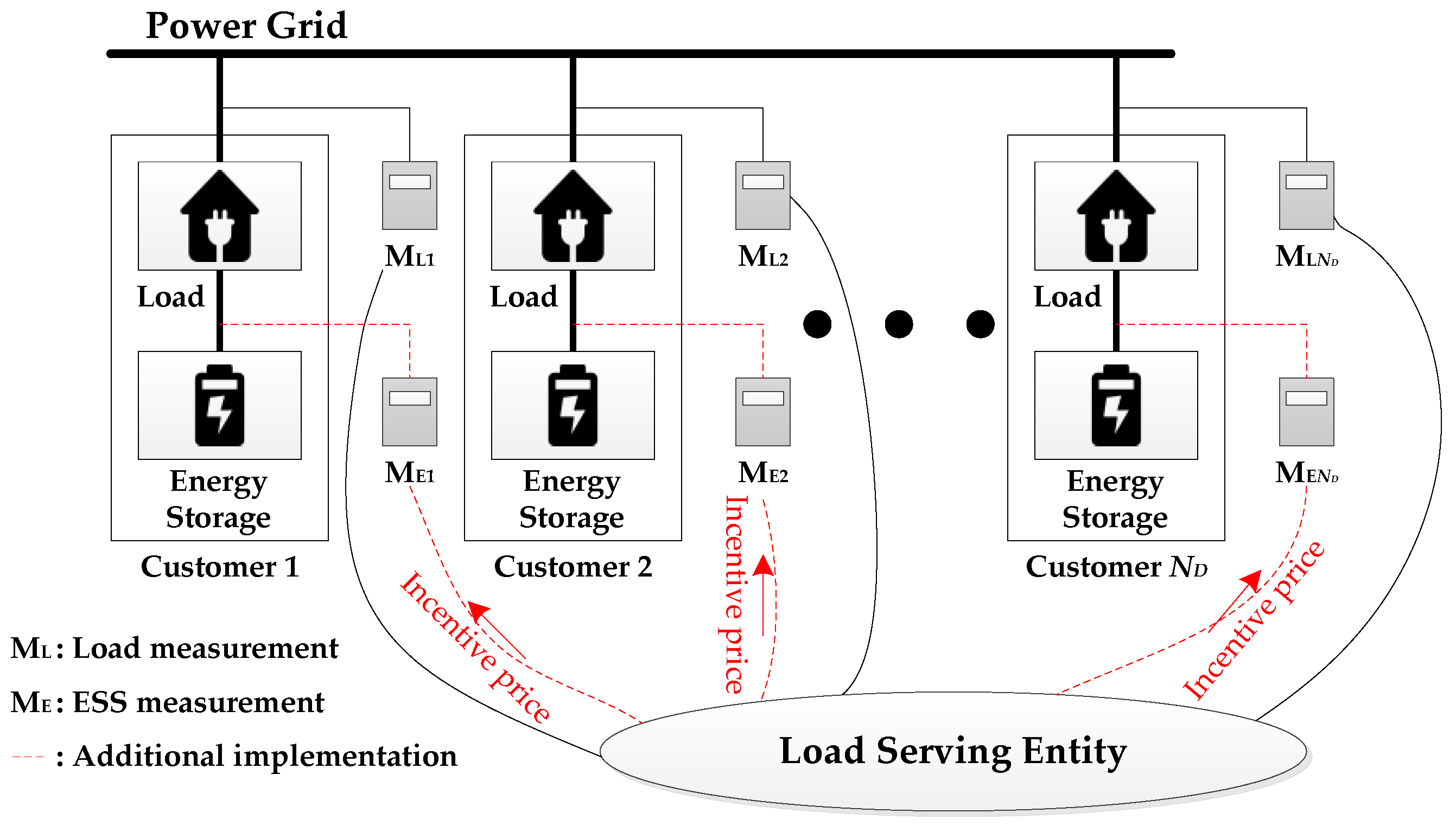
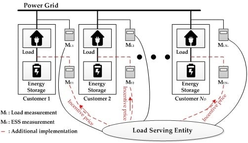
It is assumed that the number of customers owning the ESS is five. The detailed specification of the ESS is shown in

Table 1. Detailed specification of the ESS.

Customer	1	2	3	4	5
Capacity (kWh)	60	60	60	60	60
Maximum discharging power (kW)	27	24	21	18	15
Maximum charging power (kW)	27	24	21	18	15
Maximum SOC (%)	100	100	100	100	100
Minimum SOC (%)	10	12.5	15	17.5	20
Discharging Efficiency (%)	95	95	95	95	95
Charging Efficiency (%)	95	95	95	95	95
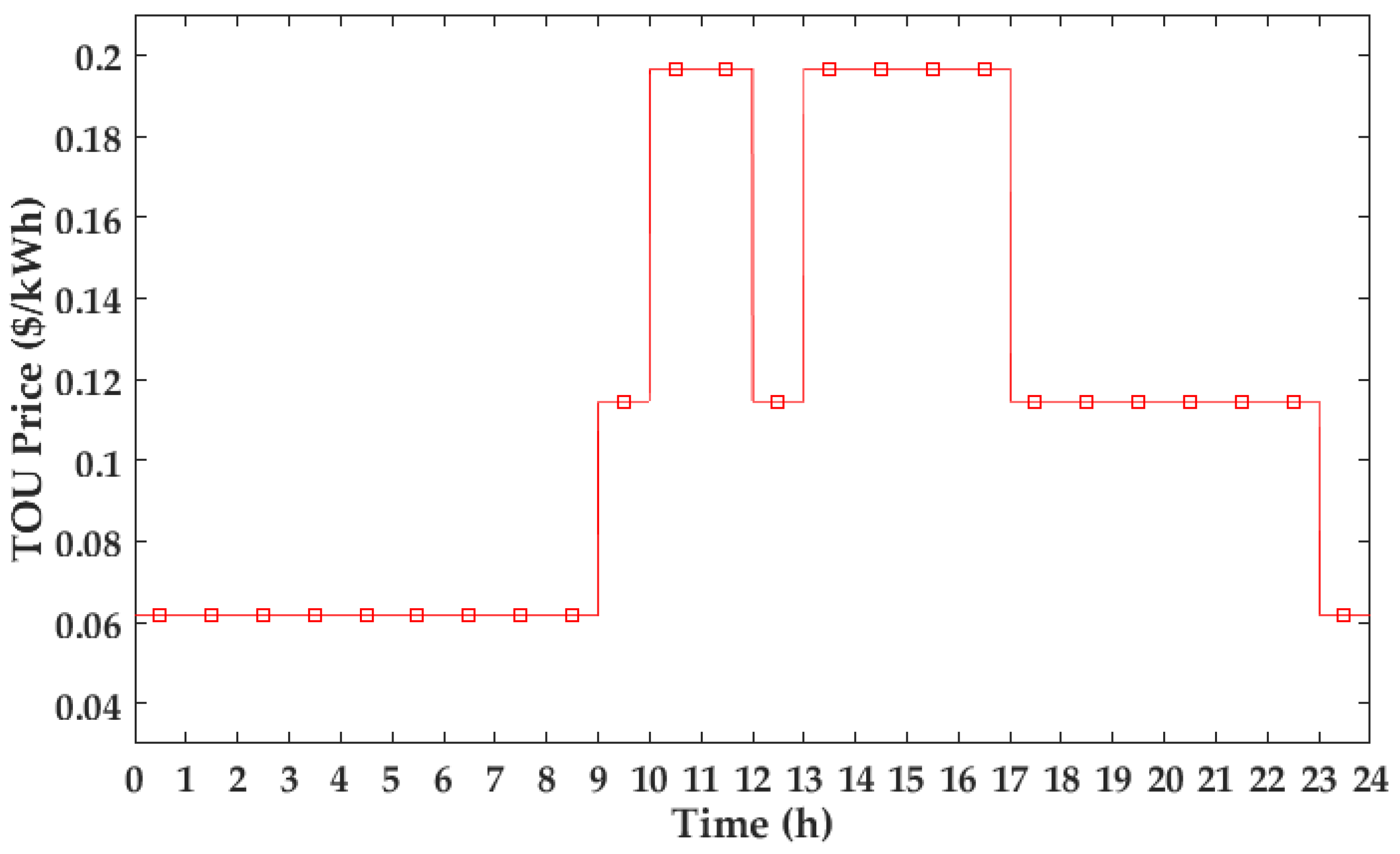
Initial SOC (%)	10	12.5	15	17.5	20

. The retail price in TOU tariff is determined depending on time and season. The TOU tariff in summer is shown in Figure 5 and these are obtained from Korea electric power corporation website [25]. The tariff is divided into three level prices. The peak time periods are 10:00–12:00 and 13:00–17:00. The off-peak time period is 23:00–9:00. The remaining are the mid-peak times.

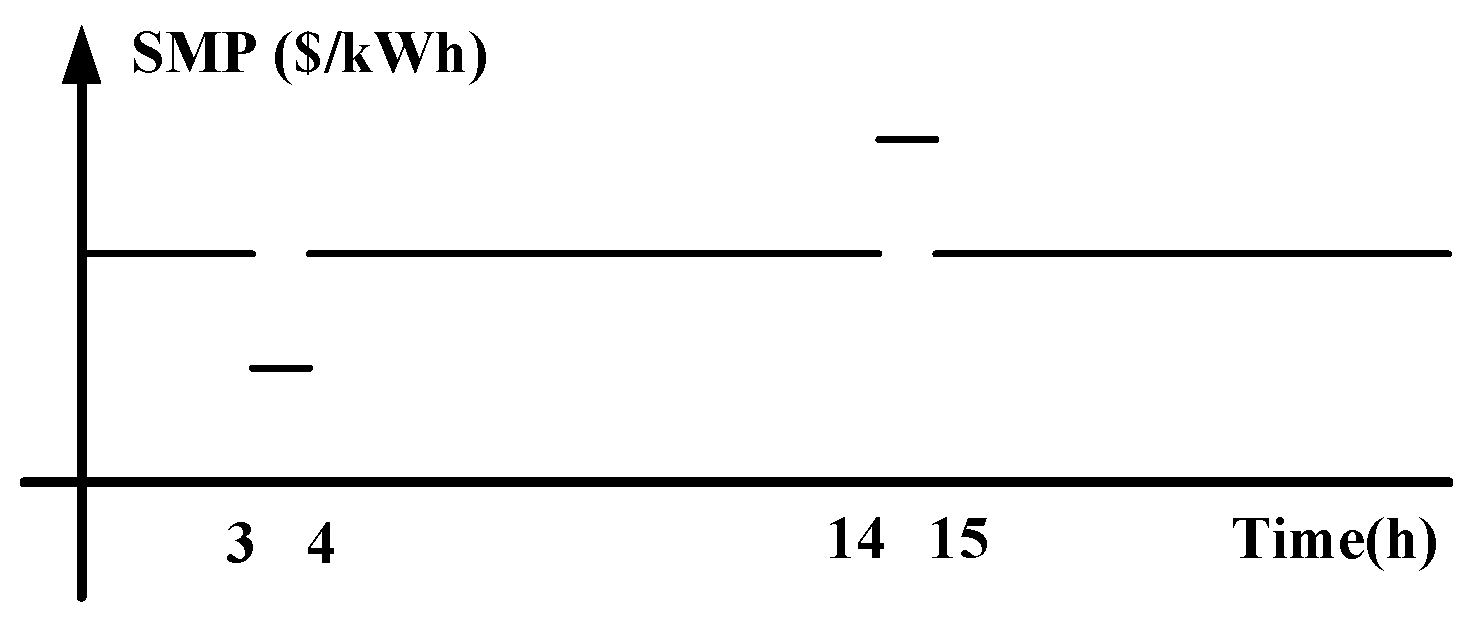
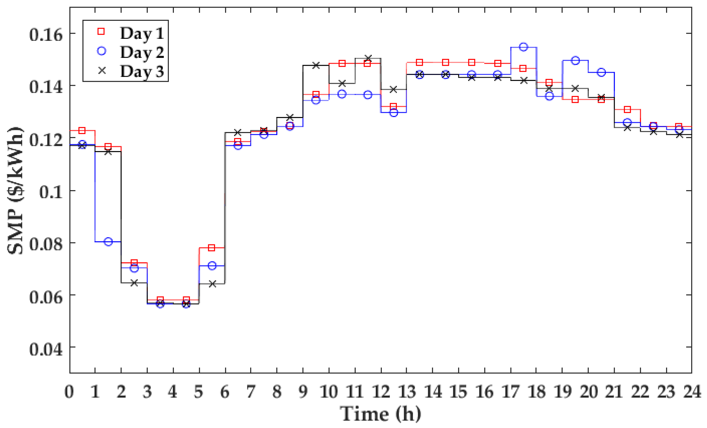
The three-day SMP data are obtained from Electric power statistics information system website, as shown in Figure 6 [26]. These are the weekday SMPs in summer. On Day 1, the SMPs are high when the TOU price is the peak-time price. On Day 2, the SMPs are high after 13:00 and the SMP from 12:00 to 13:00 is slightly different from the SMPs before 12:00. On Day 3, the SMPs are high during 9:00–10:00 and 11:00–12:00 and the SMP from 12:00 to 13:00 is slightly different from the SMPs after 13:00. Further, the SMPs from 3:00 to 5:00 are the lowest on these three days.

In order to satisfy the mathematical problem with equilibrium, the penalty parameter, π, is set to a large value. In this paper, the penalty parameter is set to 100. The minimum and maximum acceptable incentive prices are set to 0 ($/kWh) and 0.14 ($/kWh), respectively, because the unit of incentive price is kept within the unit of other prices, that is, TOU and SMP.

To identify the effect of the proposed incentive scheme, the following three case studies were simulated and the results were compared. Because the schedule is determined by the customer and not the LSE, it is possible that the customer determines the ESS charging schedule irrespective of the incentive pricing signal. Case 3 identifies this effect:

Case 1 

The customer determines the ESS charging schedule based on the TOU tariff, and there is no incentive.

Case 2 

The incentive pricing signal is determined by the proposed method when r is set to 0.5. The signal is sent to the customers. The customer determines the ESS charging schedule based on the TOU tariff and the incentive pricing signal.

Case 3 

The incentive pricing signal is equal to the incentive in Case 2. The signal is sent to the customers. However, the customer determines the ESS charging schedule based on the only TOU tariff. In other words, the ESS charging schedule is equal to the ESS charging schedule in Case 1.

5.2. Test Results

As explained in Section 4.4, because the TOU tariff follows three-level pricing rates, the optimal ESS charging schedule is indeterminate. In order to determine the optimal ESS charging schedule in Cases 1 and 3, the objective Equation (37), is modified by Equation (42):

$$\underset{{P_{\text{ESS},i,t}}^{+},{P_{\text{ESS},i,t}}^{-}}{\min }\left({\displaystyle \sum _{t=1}^{N_{\mathrm{T}}}\left(-C_{\mathrm{R},t}\left({P_{\text{ESS},i,t}}^{+}-{P_{\text{ESS},i,t}}^{-}\right)\right)}+w{\displaystyle \sum _{t=1}^{N_{\mathrm{T}}}{\left(P_{\mathrm{d},i,t}-{P_{\text{ESS},i,t}}^{+}+{P_{\text{ESS},i,t}}^{-}\right)}^2}\right)$$

(42)

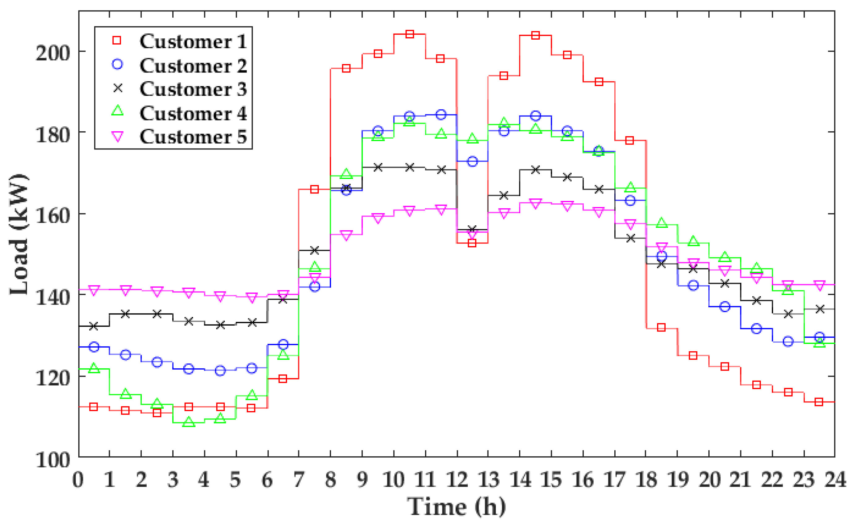
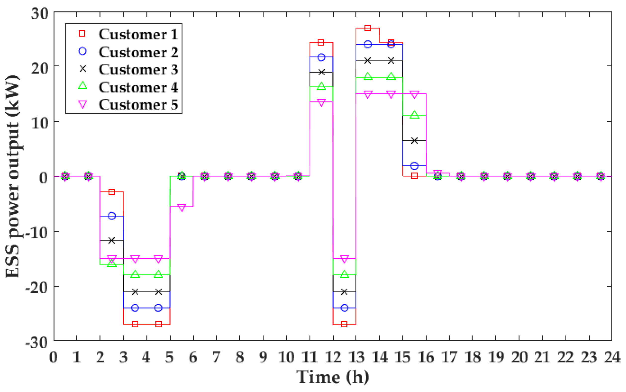
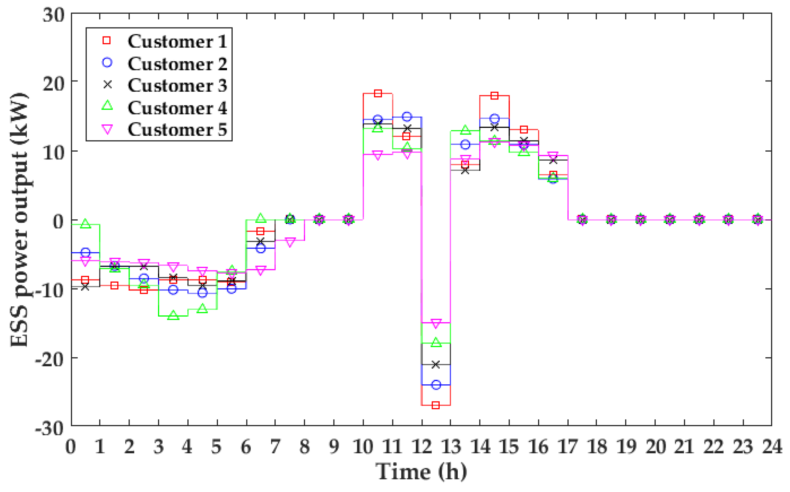
The constraints are Equations (20), (21), and (23). The additional term is related with the peak-to-average ratio. Further, w is set to 0.000001. Owing to small w, the charging periods and discharging periods are determined by TOU price dominantly. It is assumed that the load demands of customers are shown in Figure 7. The ESS charging schedules in Cases 1 and 3 during the three days are fixed as shown in Figure 8 because the TOU tariff is fixed. The discharging period is the peak time period and the charging periods are two time periods. One is the off-peak time period and the other is the mid-peak time between 12:00 and 13:00. Further, because of the additional term, more electricity is discharged when the load demand is higher during the discharging periods and more electricity is charged when the load demand is lower during the charging periods.

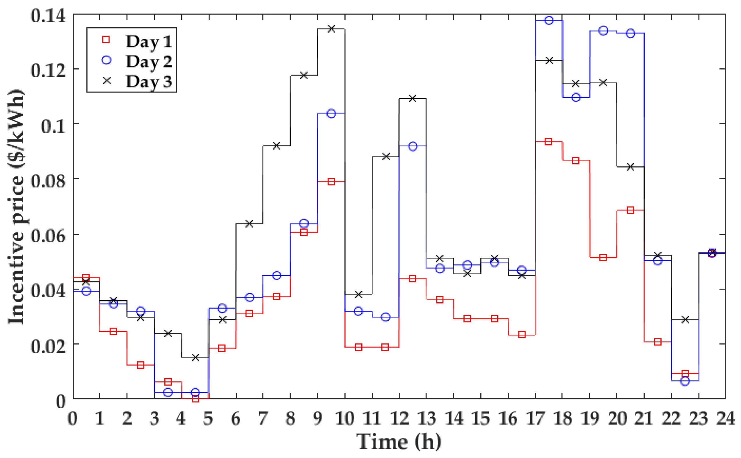
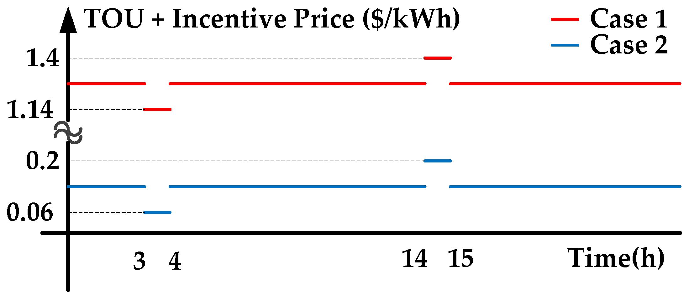
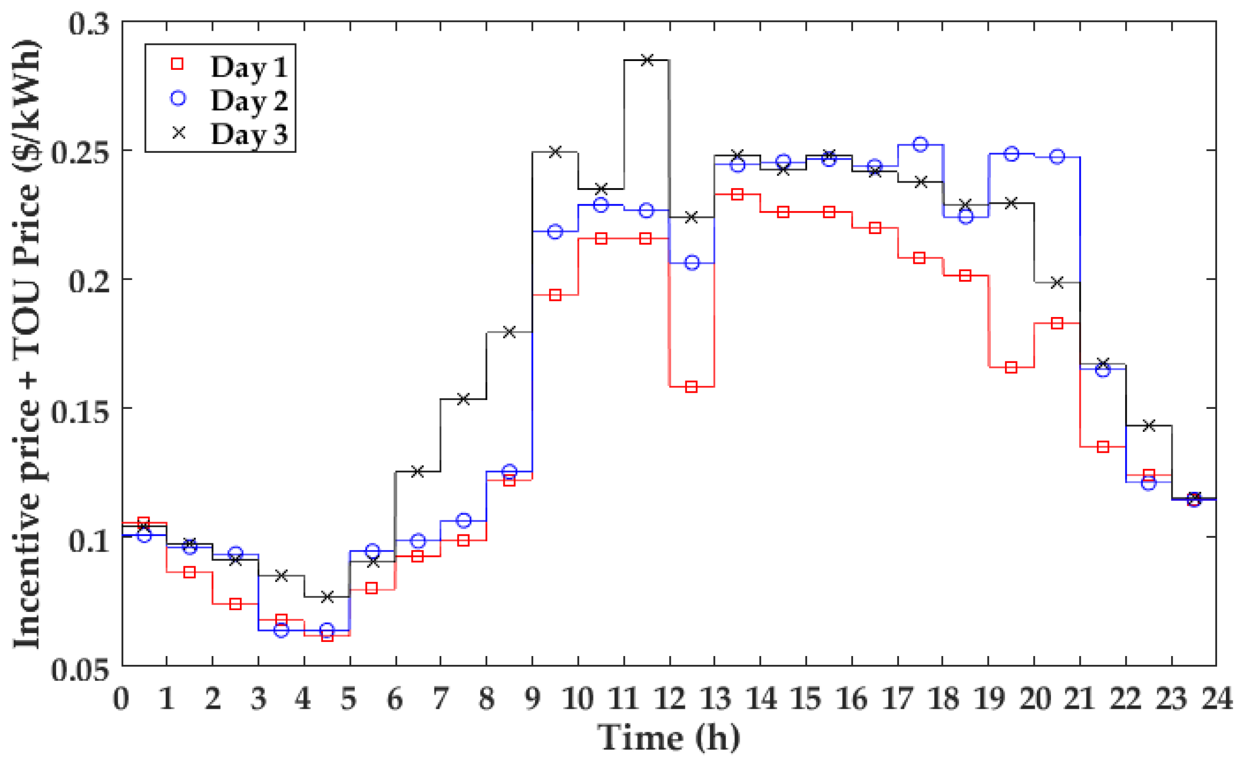
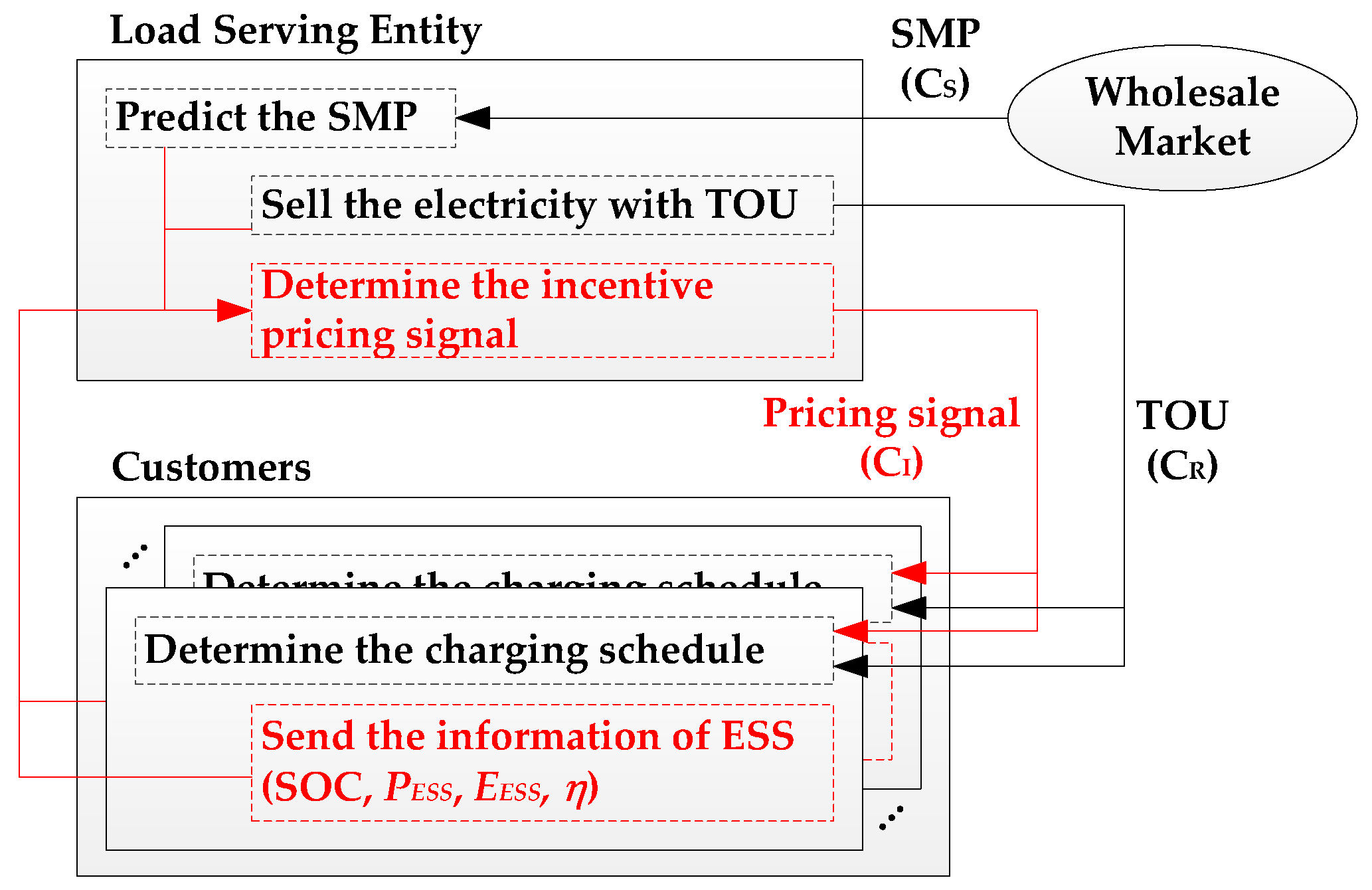
The three-day incentive prices in Cases 2 and 3 are shown in Figure 9. The sums of incentive prices and TOU prices are shown in Figure 10. The customers determine the ESS charging schedule based on these sums. In the proposed scheme, if the SMP is higher, the sum of the incentive price and TOU is also higher. Therefore, it seems that the customers determine the ESS charging schedules based on the SMP, although they use the TOU rates.

The ESS charging schedules of Case 2 on Days 1, 2 and 3 are shown in Figure 11, Figure 12 and Figure 13, respectively.

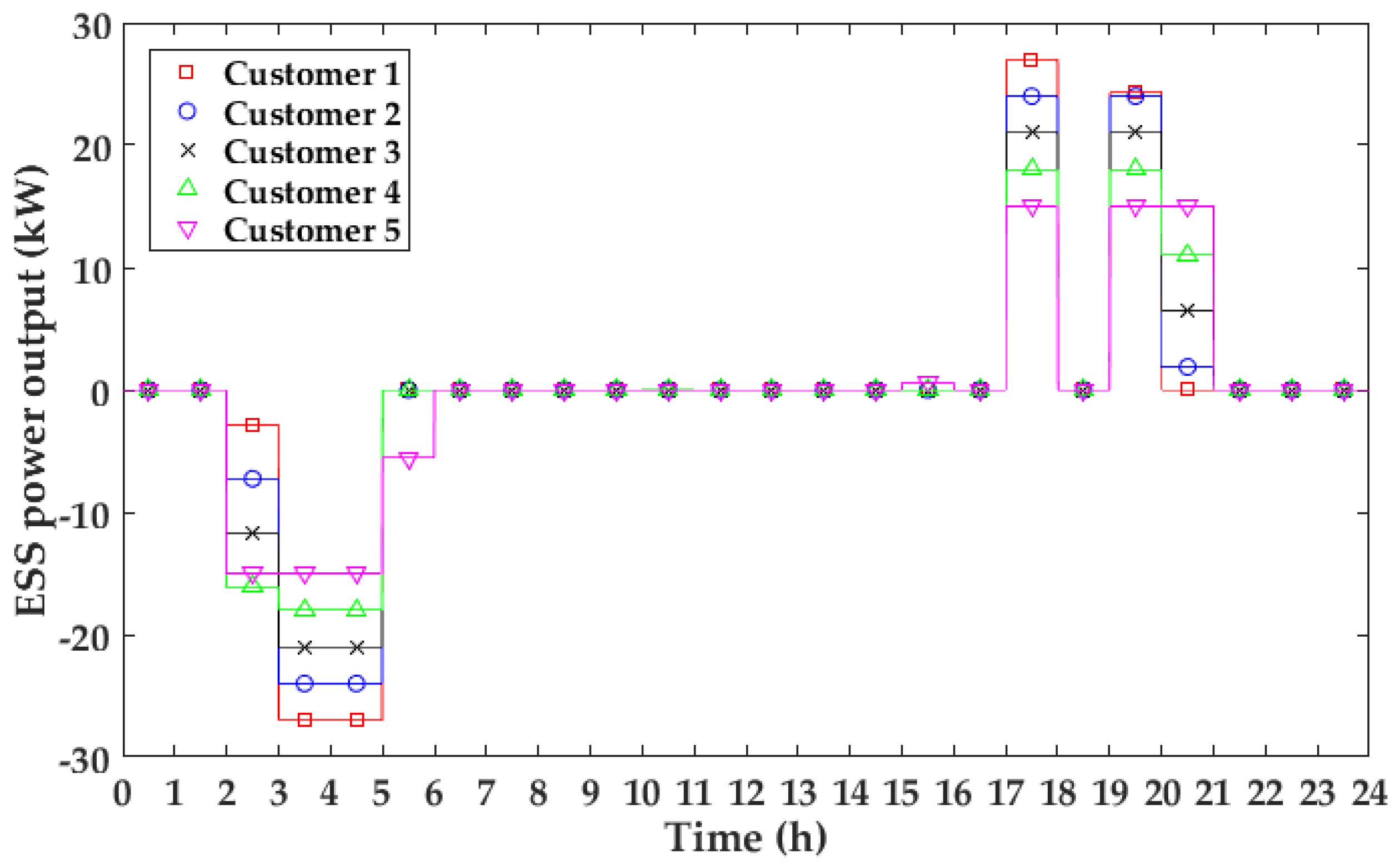
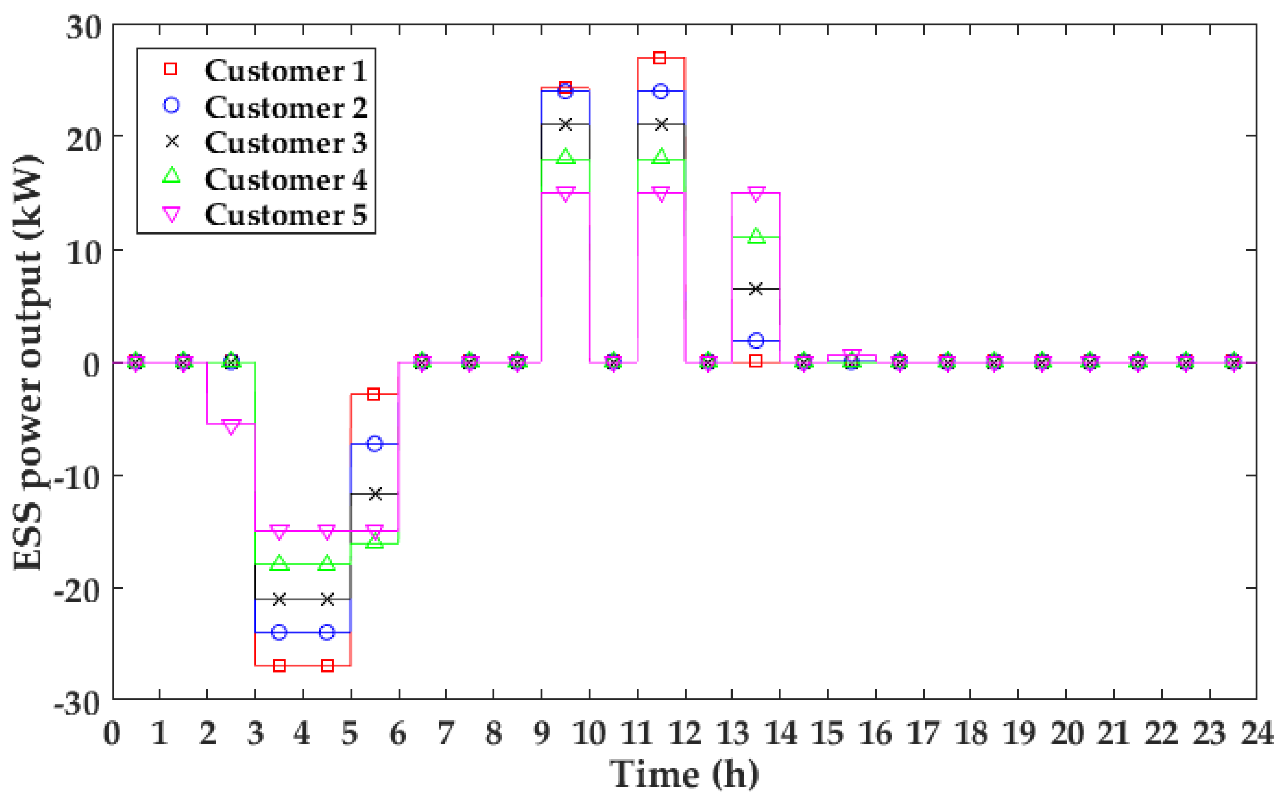
The incentive prices are lower from 3:00 to 5:00 than at other off-peak times as shown in Figure 6, because the SMPs are the lowest among the off-peak time periods. Therefore, the ESSs charge the electricity during these times intensively. On Day 1, the SMP from 12:00 to 13:00 is sufficiently low compared to the SMPs in the peak time. Therefore, it is efficient to charge the electricity in this time period. On Day 2, because of little difference between SMP from 12:00 to 13:00 and SMPs before 12:00, charging the electricity during this time is improper to increase the cost savings from the wholesale market upon considering the charging and discharging efficiency. Similarly, on Day 3, charging the electricity from 12:00 to 13:00 is not efficient because of little difference between SMP in this time period and SMPs after 13:00. Therefore, the ESSs charge the electricity during this time period on Day 1 but the ESSs do not charge the electricity during this time period on Day 2 and Day 3 in the proposed incentive scheme.

The discharging times are determined as the time periods when the SMPs are high on three days, which are during 10:00–12:00 and 13:00–17:00 on Day 1, 17:00–18:00 and 19:00–21:00 on Day 2 and 9:00–10:00 and 11:00–12:00 on Day 3. The remaining energy caused by the limitation of discharging power is discharged when SMP is the highest among the remaining time periods, because the sum of the incentive price and TOU price is also the highest in the proposed method.

The profits of all customers and losses of the LSE are summarized for each of the three days in

Table 2. Total profit and loss on Day 1 (unit: $). LSE: load-serving entity.

Case	Customer Profit			LSE Loss				Social Welfare
	Cost Savings 1	Incentive Payments	Total	Revenue Loss	Expenditure for Incentive	Cost Savings 2	Total
1	37.72	0	37.72	−37.72	0	13.86	−23.86	13.86
2	37.69	3.59	41.28 (9.44%)	−37.69	−3.59	19.74	−21.54 (9.72%)	19.74 (42.42%)
3	37.72	−0.44	37.28 (–1.17%)	−37.72	0.44	13.86	−23.42 (1.84%)	13.86 (0.00%)

¹ Cost savings from the retail market. ² Cost savings from the wholesale market.

,

Table 3. Total profit and loss on Day 2 (unit: $).

Case	Customer Profit			LSE Loss				Social Welfare
	Cost Savings 1	Incentive Payments	Total	Revenue Loss	Expenditure for Incentive	Cost Savings 2	Total
1	37.72	0	37.72	−37.72	0	13.71	−24.01	13.71
2	11.29	30.32	41.61 (10.31%)	−11.29	−30.32	20.63	−20.98 (12.62%)	20.63 (50.47%)
3	37.72	−1.77	35.95 (−4.69%)	−37.72	1.77	13.71	−22.24 (7.37%)	13.71 (0.00%)

¹ Cost savings from the retail market. ² Cost savings from the wholesale market.

and

Table 4. Total profit and loss on Day 3 (unit: $).

Case	Customer Profit			LSE Loss				Social Welfare
	Cost Savings 1	Incentive Payments	Total	Revenue Loss	Expenditure for Incentive	Cost Savings 2	Total
1	37.72	0	37.72	−37.72	0	12.97	−24.75	12.97
2	22.71	19.00	41.71 (10.58%)	−22.71	–19.00	20.23	−21.48 (13.21%)	20.23 (55.98%)
3	37.72	−1.73	35.99 (−4.59%)	−37.72	1.73	12.97	−23.02 (6.99%)	12.97 (0.00%)

¹ Cost savings from the retail market. ² Cost savings from the wholesale market.

, respectively. The customer profits in Table 2, Table 3 and Table 4 are the sum of the profits of all customers, and the detailed profit of the individual customer is presented in

Table A1. Profit of customers on Day 1 (unit: $).

Customer	Case	Cost Savings	Incentive Payments	Total	Customer	Case	Cost Savings	Incentive Payments	Total
1	1	8.29	0	8.29	2	1	7.95	0	7.95
	2	8.28	0.76	9.04		2	7.92	0.74	8.66
	3	8.29	−0.3	7.99		3	7.95	−0.09	7.86
3	1	7.53	0	7.53	4	1	7.16	0	7.16
	2	7.54	0.73	8.27		2	7.17	0.71	7.88
	3	7.53	−0.22	7.31		3	7.16	0.3	7.46
5	1	6.79	0	6.79	Total	1	37.72	0	37.72
	2	6.78	0.65	7.43		2	37.69	3.59	41.28
	3	6.79	−0.13	6.66		3	37.72	−0.44	37.28

,

Table A2. Profit of customers on Day 2 (unit: $).

Customer	Case	Cost Savings	Incentive Payments	Total	Customer	Case	Cost Savings	Incentive Payments	Total
1	1	8.29	0	8.29	2	1	7.95	0	7.95
	2	2.39	6.73	9.12		2	2.32	6.41	8.73
	3	8.29	−0.74	7.55		3	7.95	−0.48	7.47
3	1	7.53	0	7.53	4	1	7.16	0	7.16
	2	2.24	6.09	8.33		2	2.18	5.74	7.92
	3	7.53	−0.44	7.09		3	7.16	0.1	7.26
5	1	6.79	0	6.79	Total	1	37.72	0	37.72
	2	2.16	5.35	7.51		2	11.29	30.32	41.61
	3	6.79	−0.21	6.58		3	37.72	−1.77	35.95

and

Table A3. Profit of customers on Day 3 (unit: $).

Customer	Case	Cost Savings	Incentive Payments	Total	Customer	Case	Cost Savings	Incentive Payments	Total
1	1	8.29	0	8.29	2	1	7.95	0	7.95
	2	4.59	4.51	9.10		2	4.43	4.28	8.71
	3	8.29	−0.72	7.57		3	7.95	−0.36	7.59
3	1	7.53	0	7.53	4	1	7.16	0	7.16
	2	4.5	3.84	8.34		2	4.58	3.41	7.99
	3	7.53	−0.34	7.19		3	7.16	0.08	7.24
5	1	6.79	0	6.79	Total	1	37.72	0	37.72
	2	4.61	2.96	7.57		2	22.71	19.00	41.71
	3	6.79	−0.39	6.4		3	37.72	−1.73	35.99

of Appendix.

The profit and the loss related with the constant load demand are eliminated in the Tables. The cost savings of the customer is the cost savings from the retail prices and the cost savings of the LSE is the cost savings from the wholesale prices. The social welfare is equal to the cost savings from the wholesale market. The values in parentheses denote the ratio of increase in the profit and the ratio decrease in the loss compared to Case 1. Because the customers use the ESS for the purpose of the cost savings in the TOU scheme, the revenue of the LSE from the retail market decreases. Therefore, the total LSE profit caused by the ESS is negative and is described as the loss. Further, if the expenditure for incentive is negative, the LSE gives the incentive to customers. Otherwise, the bill of the customer increases.

In the incentive scheme using the proposed method, the social welfare increased compared only to the TOU scheme. In addition, the profit of the customer increased and the loss of the LSE decreased.

In Case 2, owing to setting r to 0.5, more than 50% of increased social welfare compared to Case 1 is given to the customers. The portions of the customers for the increased social welfare on Day 1, Day 2, and Day 3 are 60.54%, 56.21%, and 54.96%, respectively. In order to verify the effect of r, r changes from 0.1 to 0.9 and the interval is 0.2. The portions of the total customers for the increased social welfare on Day 1, Day 2, and Day 3 are shown in

Table 5. Portion of the customers for the increased social welfare.

r	0.1	0.3	0.5	0.7	0.9
Day 1	12.82%	36.63%	60.54%	79.58%	97.10%
Day 2	11.85%	34.68%	56.21%	79.94%	91.76%
Day 3	11.57%	35.12%	54.96%	74.34%	98.90%

. Because the LSE increases its portions and the minimum ratio is maintained by Equation (41), the portion of the customer is close to r. Therefore, the increased social welfare can be divided by the intention of the LSE. Further, when r is set to 0.5, the portion of all customers is similar to the portion of the LSE.

On the other hand, as shown in Cases 2 and 3, when the customer determines the ESS charging schedule irrespective of the incentive pricing signal, the profit of the customer is reduced. Therefore, in order to maximize the profit, the customer considers the incentive price when it determines the ESS charging schedule.

Therefore, the social welfare is increased and the profit can be divided into the LSE and the customers equitably in the proposed incentive scheme. In addition, the customer follows the intention of the LSE to maximize his/her profit from the incentive scheme.

6. Conclusions

In general, the TOU tariff divided into three level prices is the most popular tariff as a price-based ILC. Because the TOU rates do not change variously contrary to the wholesale market price, the ESS operation determined by customer for reducing its energy cost does not effectively reflect the wholesale market price.

In order to maximize the ESS utilization, ILC using the incentive price for the ESS operation is proposed under the TOU tariff. An additional meter that measures the ESS operation is implemented at the ESS owned by the customer and the LSE sends the incentive pricing signal for the ESS operation. Because the ESS charging schedule is determined by the optimization problem of the customer, the bilevel optimization problem is utilized for determining the incentive pricing signal in this paper. In order to solve the bilevel optimization problem by using an interior point method, the bilevel optimization problem is reformulated into a one-level problem in which the objective function and all the constraints are twice differentiable. This is done by reformulating the piecewise linear constraint to linear constraint, adjusting the KKT conditions of the LLP, and using the penalty methods.

The proposed incentive scheme increases the social welfare compared to the TOU rates. In addition, the increased social welfare is divided into the LSE and the customer equitably. Further, the proposed incentive scheme leads the customer to follow the signal voluntarily, because the customer desires to maximize his/her profit.

References

1. Ogwumike, C.; Short, M.; Abugchem, F. Heuristic optimization of consumer electricity costs using a generic cost model. Energies 2016, 9, 6. [Google Scholar] [CrossRef]
2. Iglesias, F.; Palensky, P.; Cantos, S.; Kupzog, F. Demand side management for stand-alone hybrid power systems based on load identification. Energies 2012, 5, 4517–4532. [Google Scholar] [CrossRef]
3. Guo, Y.; Pan, M.; Fang, Y.; Khargonekar, P.P. Decentralized coordination of energy utilization for residential households in the smart grid. IEEE Trans. Smart Grid 2013, 4, 1341–1350. [Google Scholar] [CrossRef]
4. Kostkova, K.; Omelina, L.; Kycina, P.; Jamrich, P. An introduction to load management. Electr. Power Syst. Res. 2013, 95, 184–191. [Google Scholar] [CrossRef]
5. Yoo, T.H.; Park, H.; Park, J.-K. Determining the interruptible load with strategic behavior in a competitive electricity market. Energies 2015, 8, 257–277. [Google Scholar] [CrossRef]
6. Faruqui, A.; George, S.S. The value of dynamic pricing in mass markets. Electr. J. 2002, 15, 45–55. [Google Scholar] [CrossRef]
7. Joskow, P.; Tirole, J. Retail electricity competition. Rand J. Econ. 2006, 37, 799–815. [Google Scholar] [CrossRef]
8. Celebi, E.; Fuller, J.D. A model for efficient consumer pricing scheme in electricity markets. IEEE Trans. Power Syst. 2007, 22, 60–67. [Google Scholar] [CrossRef]
9. Hu, Z.; Kim, J.H.; Wang, J.; Byrne, J. Review of dynamic pricing programs in the U.S. and Europe: Status quo and policy recommendations. Renew. Sustain. Energy Rev. 2015, 42, 743–751. [Google Scholar] [CrossRef]
10. Nguyen, H.K.; Song, J.B.; Han, Z. Distributed demand side management with energy storage in smart grid. IEEE Trans. Parallel Distrib. Syst. 2015, 26, 3346–3357. [Google Scholar] [CrossRef]
11. Jiang, T.; Cao, Y.; Yu, L.; Wang, Z. Load shaping strategy based on energy storage and dynamic pricing in smart grid. IEEE Trans. Smart Grid 2014, 5, 2868–2876. [Google Scholar] [CrossRef]
12. Soliman, H.M.; Leon-Garcia, A. Game-theoretic demand-side management with storage devices for the future smart grid. IEEE Trans. Smart Grid 2014, 5, 1475–1485. [Google Scholar] [CrossRef]
13. Daryanian, B.; Tabors, R.D.; Bohn, R.E. Optimal demand-side response to electricity spot price for storage-type customers. IEEE Trans. Power Syst. 1989, 4, 897–903. [Google Scholar] [CrossRef]
14. Daryanian, B.; Bohn, R.E.; Tabors, R.D. An experiment in real time pricing for control of electric thermal storage systems. IEEE Trans. Power Syst. 1991, 6, 1356–1365. [Google Scholar] [CrossRef]
15. Lee, T.Y.; Chen, N. Determination of optimal contract capacities and optimal sizes of battery energy storage systems for time-of-use rates industrial customers. IEEE Trans. Energy Convers. 1995, 10, 562–568. [Google Scholar]
16. Lee, T.Y. Operating schedule of battery energy storage system in a time-of-use rate industrial user with wind turbine generators: A multipass iteration particle swarm optimization approach. IEEE Trans. Energy Convers. 2007, 22, 774–782. [Google Scholar] [CrossRef]
17. Wang, Z.; He, Y. Two-stage optimal demand response with battery energy storage systems. IET Gener. Transm. Distrib. 2016, 10, 1286–1293. [Google Scholar] [CrossRef]
18. Kilkki, O.; Alahaivala, A.; Seilonen, I. Optimized control of price-based demand response with electric storage space heating. IEEE Trans. Ind. Inform. 2015, 11, 281–288. [Google Scholar] [CrossRef]
19. Gungor, V.C.; Sahin, D.; Kocak, T.; Ergut, S.; Buccella, C.; Cecati, C.; Hancke, G.P. Smart grid technologies: Communication technologies and standards. IEEE Trans. Ind. Inform. 2011, 7, 529–539. [Google Scholar] [CrossRef]
20. Siano, P. Demand response and smart grids—A survey. Renew. Sustain. Energy Rev. 2014, 30, 461–478. [Google Scholar] [CrossRef]
21. Boyd, S.; Vandenberghe, L. Convex Optimization; Cambridge University Press: Cambridge, UK, 2004; pp. 561–562. [Google Scholar]
22. Case, L.M. An l1 Penalty Function Approach to the Nonlinear Bilevel Programming Problem. Ph.D. Thesis, University of Waterloo, Waterloo, ON, Canada, 1997. [Google Scholar]
23. Andreani, R.; Haeser, G.; Schuverdt, M.L.; Silva, P.J. A relaxed constant positive linear dependence constraint qualification and applications. Math. Program. 2012, 135, 255–273. [Google Scholar] [CrossRef]
24. Benson, H.Y.; Sen, A.; Shannon, D.F.; Vanderbei, R.J. Interior-point algorithms, penalty methods and equilibrium problems. Comput. Optim. Appl. 2006, 34, 155–182. [Google Scholar] [CrossRef]
25. Korea Electric Power Corporation. Available online: http://home.kepco.co.kr/kepco/EN/F/htmlView/ENFBHP00102.do?menuCd=EN060201 (accessed on 29 March 2016).
26. Electric Power Statistics Information System. Available online: http://epsis.kpx.or.kr/epsis/ekmaStaticMain.do?cmd=004013&flag=&locale=EN (accessed on 29 March 2016).
Figure 1. System model for the proposed indirect load control (ILC). ESS: energy storage system.
Energies 09 00558 g001
Figure 2. Process of determining the ESS charging schedule. SMP: system marginal price; TOU: time-of-use; and SOC: state of charge.
Energies 09 00558 g002
Figure 3. SMP profile for example.
Energies 09 00558 g003
Figure 4. Two cases of sums of incentive prices and time-of-use (TOU) prices.
Energies 09 00558 g004
Figure 5. TOU tariff in summer.
Energies 09 00558 g005
Figure 6. SMP profile for three days.
Energies 09 00558 g006
Figure 7. Load demand profile.
Energies 09 00558 g007
Figure 8. ESS charging schedule based on the TOU tariff.
Energies 09 00558 g008
Figure 9. Incentive prices in Cases 2 and 3.
Energies 09 00558 g009
Figure 10. Sums of incentive prices and TOU prices.
Energies 09 00558 g010
Figure 11. ESS charging schedule in Case 2 on Day 1.
Energies 09 00558 g011
Figure 12. ESS charging schedule in Case 2 on Day 2.
Energies 09 00558 g012
Figure 13. ESS charging schedule in Case 2 on Day 3.
Energies 09 00558 g013