Article

A Novel Method to Magnetic Flux Linkage Optimization of Direct-Driven Surface-Mounted Permanent Magnet Synchronous Generator Based on Nonlinear Dynamic Analysis

1
State Key Laboratory of Electrical Insulation and Power Equipment, School of Electrical Engineering, Xi’an Jiaotong University, Xi’an 710049, China
2
Institute of Water Resources and Hydro-electric Engineering, Xi’an University of Technology, Xi’an 710048, China
*
Author to whom correspondence should be addressed.
Energies 2016, 9(7), 557; https://doi.org/10.3390/en9070557
Submission received: 19 June 2016 / Revised: 8 July 2016 / Accepted: 9 July 2016 / Published: 19 July 2016

Abstract

:
This paper pays attention to magnetic flux linkage optimization of a direct-driven surface-mounted permanent magnet synchronous generator (D-SPMSG). A new compact representation of the D-SPMSG nonlinear dynamic differential equations to reduce system parameters is established. Furthermore, the nonlinear dynamic characteristics of new D-SPMSG equations in the process of varying magnetic flux linkage are considered, which are illustrated by Lyapunov exponent spectrums, phase orbits, Poincaré maps, time waveforms and bifurcation diagrams, and the magnetic flux linkage stable region of D-SPMSG is acquired concurrently. Based on the above modeling and analyses, a novel method of magnetic flux linkage optimization is presented. In addition, a 2 MW D-SPMSG 2D/3D model is designed by ANSYS software according to the practical design requirements. Finally, five cases of D-SPMSG models with different magnetic flux linkages are simulated by using the finite element analysis (FEA) method. The nephograms of magnetic flux density are agreement with theoretical analysis, which both confirm the correctness and effectiveness of the proposed approach.

Graphical Abstract

1. Introduction

In wind energy applications, variable speed wind turbines have many advantages over fixed-speed generation such as increased energy capture, operation at maximum power point, improved efficiency, and power quality [1,2]. Presently, doubly fed induction generators (DFIGs) are widely used as the generators in a variable speed wind turbine system. In the case of DFIGs, there is a requirement for the gearbox to match the turbine and rotor speed. The gearbox often suffers from faults and requires regular maintenance, making the system unreliable [3]. The reliability of the variable-speed wind turbine can be improved significantly by using a direct-driven surface-mounted permanent magnet synchronous generator (D-SPMSG). D-SPMSG has received much attention in wind-energy application because of its property of self-excitation, which allows an operation at a high power factor and high efficiency [4,5]. The use of a permanent magnet in the rotor of the D-SPMSG makes it unnecessary to supply magnetizing current through the stator for constant air-gap flux; the stator current needs only to be torque producing [6]. Hence, for the same output, the D-SPMSG will operate at a higher power factor because of the absence of the magnetizing current and will be more efficient than other machines [7].
It is well known that the existing mathematical models of generators are multi-variable, nonlinear, and strongly coupled; therefore, these systems can exhibit complex behaviors [8,9,10,11]. It is now a common belief that understanding and utilizing the rich dynamics, such as bifurcations and chaos, of nonlinear systems have an important impact on the modern technology [12,13,14,15,16]. A D-SPMSG is a kind of high-efficient and high-powered generator, and there are still some problems in the D-SPMSG, which exhibits chaotic behavior when parameters of the D-SPMSG are changed or have some special operating conditions [17,18]. The chaotic behavior in D-SPMSG is undesirable since it can degrade the performance of, and even destroy the stability of the generator and make the system collapse. With the development of permanent-magnet materials, the unique advantage of D-SPMSG is increasingly evident and it is widely used in wind power systems [19,20]. In this pursuit, however, research on bifurcation and chaotic phenomena of the D-SPMSG is still behind the rapidly evolving trend of nonlinear sciences and engineering.
In this paper, we have analyzed the influence of magnetic flux linkage change on D-SPMSG dynamics behavior. One representative method to optimize magnetic flux linkage is adjusting the size of the permanent magnet, thereby magnetic flux density will also be affected. Accordingly, in the process of D-SPMSG magnetic flux linkage optimization, if the value of the magnetic flux linkage is too small, it will affect the performance of the generator to reach the operational requirements, and if the value of the magnetic flux linkage is too large, it will cause unstable operation, overheating and unit vibration of D-SPMSG. Additionally, traditional design of permanent magnet size is estimated using the empirical formula, and many of the parameters in the formula are empirical values, e.g., [21], this does not guarantee the accuracy and reliability of the final design result [22,23]. Moreover, the design optimization method of permanent magnets based on analytical methods and finite element analysis is not only computationally cumbersome, but also difficult for finding the optimal solution. In recent years, some scholars adopted intelligent optimization algorithms to design the permanent magnet, which improves the overall design quality, but intelligent algorithms are not deterministic algorithms, and the establishment of specific target function is very complex, e.g., [24,25,26]. To the best of the authors’ knowledge, there are few studies on magnetic flux linkage optimization of D-SPMSG by using a nonlinear theory. Therefore, the study of magnetic flux linkage optimization becomes a necessary and important issue.
In this paper, the proposed method reduces the complexity of the system by affine transformation, and designs the permanent magnet combined with the nonlinear mathematical analysis. To contrast with the above-mentioned method, the proposed method can be achieved more easily, improves the reliability of the design and reduces the design cycle. Motivated by the above discussion, in this study, we have three advantages which make our approach attractive compared with the prior works. Firstly, by incorporating a class of transformations, a new compact form of the D-SPMSG nonlinear dynamic differential equations is established, which results in a significant reduction in the number of parameters involved, and thus, significantly reduces the complexity associated with the dynamic analysis. Secondly, by using the compact form, the nonlinear dynamic characteristics of D-SPMSG in the process of varying magnetic flux linkage is considered. Thirdly, a novel method of magnetic flux linkage optimization is proposed based on nonlinear dynamic analysis and the finite element analysis of D-SPMSG is studied in detail by using ANSYS software (Version 14.5).
The rest of the paper is organized as follows: in Section 2, a new compact form of the D-SPMSG nonlinear dynamic differential equation is established. According to the practical design requirements, a 2 MW D-SPMSG 2D/3D model is designed by ANSYS software in Section 3. Section 4 analyzes the nonlinear dynamical behaviors of the presented system in the process of magnetic flux linkage variations. In Section 5, a novel method of magnetic flux linkage optimization based on nonlinear dynamic analysis is presented and finite element analysis (FEA) is used to demonstrate the correctness and effectiveness of the proposed approach. Section 6 provides the conclusions of the paper.

2. System Modelling

2.1. Conventional Direct-Driven Surface-Mounted Permanent Magnet Synchronous Generator (D-SPMSG) for Wind Power

Usually, we use d-q rotor coordinate systems, which will synchronous rotation with rotors. Therefore, we can easily get the space vectors of D-SPMSG as shown in Figure 1. Thus, we can get the voltage equation, magnetic flux linkage equation, torque equation and motion equation as follows:
  • Voltage equations
    u d = d ψ d d t - ω e ψ q + R i d , u q = d ψ q d t + ω e ψ d + R i q ,
    where ω e = n p ω .
  • Magnetic flux linkage equations
    ψ d = L d i d + ψ f , ψ q = L q i q .
  • Torque equation
    T e = 3 2 n p ( ψ d i q - ψ q i d ) = 3 2 n p [ ( ψ f i q + ( L d - L q ) i d i q ) ] .
  • Motion equation
    J d ω d t + b ω = T w - T e .
Then, the electrical dynamics of the D-SPMSG can be expressed as:
i ˙ q = 1 L q - R i q - n p L d ω i d - n p ψ f ω + u q , i ˙ d = 1 L d - R i d + n p L q ω i q + u d , ω ˙ = 1 J T w - 1 J 3 2 n p ψ f i q + 3 2 n p ( L d - L q ) i q i d - 1 J b ω ,
the system parameters used in D-SPMSG model, as listed in Table 1.
Remark 1. 
According to the characteristics of the surface-mounted permanent magnet synchronous generator, one can obtain L q = L d .
It is obvious that the D-SPMSG system (5) under study represents highly nonlinear systems, and, in the process of design and dynamic analysis, can become greatly complex. In view of the dynamic characteristics, and due to the nature of the nonlinear system, one must include the external inputs in the parameter set. Therefore, the system dynamic characteristics can be formulated by ten parameters: ( R , L d , L q , n p , ψ f , u d , u q , T w , J , b ) .
Below, we adopt an approach to transforming the systems’ equations of motion to compact forms, whereby the number of system parameters is greatly reduced.

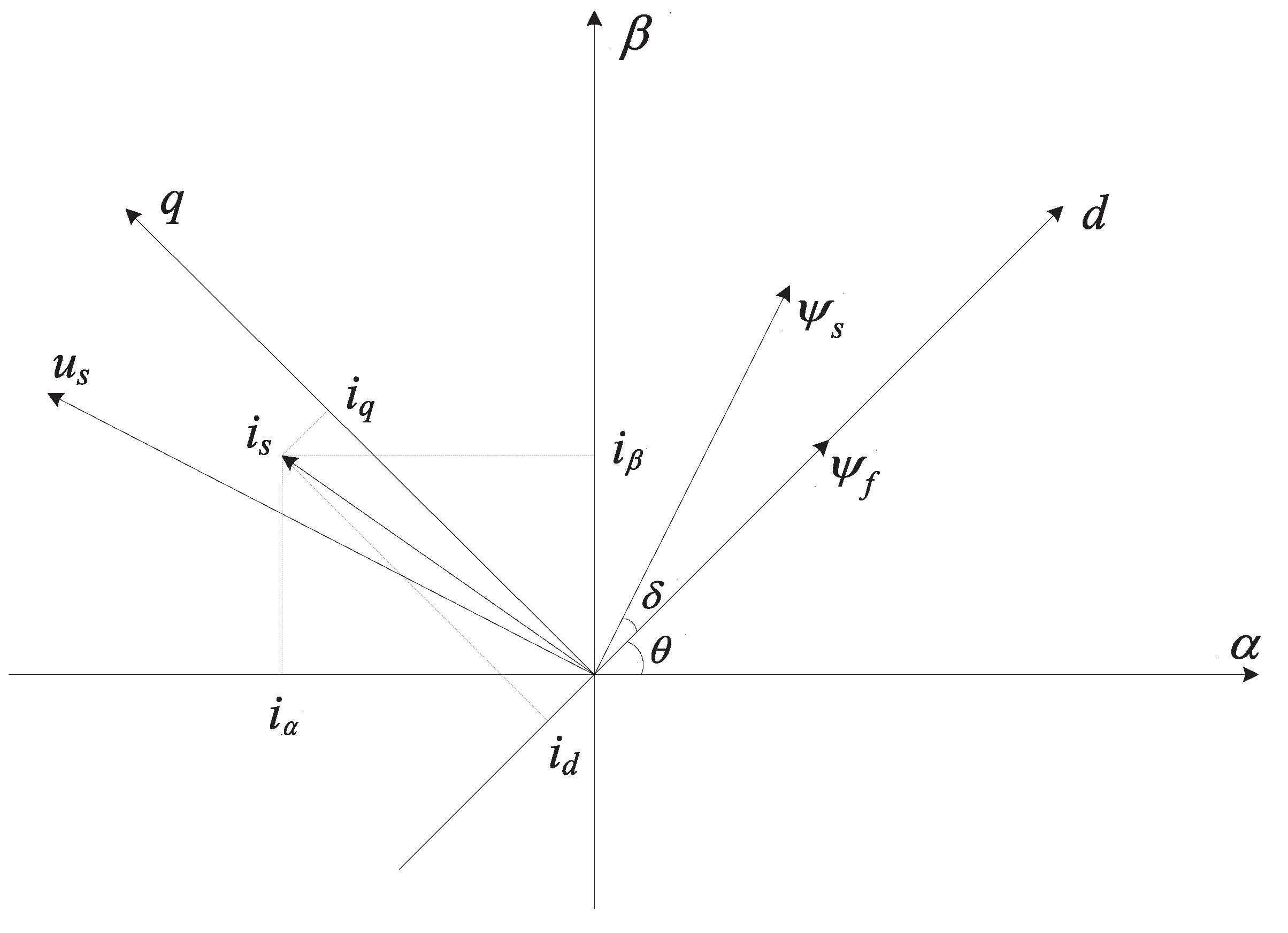
2.2. Transformation to the Compact Representation

In this section, the affine transformation method is adopted to transform the D-SPMSG Equation (5) into the new representation, which enables us to discuss the effect of the system’s dynamic behavior in a compact form. In geometry, an affine transformation is a function between affine spaces which preserves points, straight lines and planes. In addition, sets of parallel lines remain parallel after an affine transformation. An affine transformation does not necessarily preserve angles between lines or distances between points, though it does preserve ratios of distances between points lying on a straight line. An affine transformation can preserve the collinearity relation between points, the ratios of vectors along a line, and, more generally, barycenters of weighted collections of points.
To proceed, we will consider a class of transformation form described by
x = M x + Λ
where x = [ x 1 , x 2 , x 3 ] T = [ i q , i d , ω ] T are the three-dimensional state vectors of the system (5); x = [ x 1 , x 2 , x 3 ] T = [ i q , i d , ω ] T are the three-dimensional state vectors we need; M is the 3 × 3 diagonal matrix; and Λ is the 3 × 1 constant vector.
We define, M = m 1 0 0 0 m 2 0 0 0 m 3 , and Λ = λ 1 λ 2 λ 3 .
Hence, we can get
d x d t = M d x d t ,
and define another transformation as:
d x d t = N d x d t ,
where N is the 3 × 3 diagonal matrix, N = n 1 0 0 0 n 2 0 0 0 n 3 .
Theorem 1. 
The stability characteristics of the system (5) are preserved under transformations (7) and (8).
Proof of Theorem 1. 
Without loss of generality, a dynamical system described by:
d x d t = f ( x ) + g ( x ) · Δ ,
where f R n , Δ R m and g is an n × m matrix. Applying the equilibrium condition to Equation (9), we have
f ( x 0 ) + g ( x 0 ) · Δ = 0 .
Applying the transformations defined by Equation (7) and (8) to system (9), we obtain
d x d t = M - 1 N · f ( M x + Λ ) + M - 1 N · g ( M x + Λ ) · Δ = M - 1 N · f ( x ) + M - 1 N · g ( x ) · Δ .
Using the equilibrium condition to (11), we have
M - 1 N · f ( x 0 ) + M - 1 N · g ( x 0 ) · Δ = 0 .
Therefore, it is showed that the equilibrium solutions of (9) are the same as those for (11). Furthermore, the stability of the system (9) is determined by the eigenvalues of the Jacobian matrix
J = f x + g x · Δ .
For system (11), according to Equations (11) and (6), we can get the Jacobian matrix
J = f x + g x · Δ = M - 1 N · f x x x + M - 1 N · g x x x · Δ = M - 1 N · f x · M + M - 1 N · g x · M · Δ ,
which indicates that J and J are similar; accordingly, they have the same eigenvalues.
Consequently, after the transformations (7) and (8), the stability characteristics of the system (5) are preserved.   □
In order to transform the equations of motion for a conventional D-SPMSG Equation (5) to a compact form, and determine an optimum value of the magnetic flux linkage ψ f , we present the following transformation:
N = n 1 0 0 0 n 2 0 0 0 n 3 = L q R 0 0 0 L d R 0 0 0 2 b 2 3 J ,
M = m 1 0 0 0 m 2 0 0 0 m 3 = 1 b R 2 n 1 0 0 0 1 b R 2 n 2 0 0 0 1 b R n 2 ,
Λ = λ 1 λ 2 λ 3 = 0 m 2 ψ f - ψ f L d 0 .
Then, after transformations (7) and (8), we obtain
i ˙ q = - i q - μ ω i d - μ ψ f ω + u q , i ˙ d = - i d + μ ω i q + u d , ω ˙ = T w - ϑ ( μ ψ f i q + 2 3 ω ) ,
where
μ = n p b R ,
ϑ = 3 b n 3 2 J ,
u q = u q R m 1 ,
u d = u d - R λ 2 R m 2 ,
T w = 3 n 3 2 J m 3 T w .
Equation (18) constitutes a compact representation for the differential equations governing the dynamics of a conventional D-SPMSG. Comparing the original Equation (5) to the compact form Equation (18), it is obvious that the number of parameters has been reduced from ten to six. Therefore, the characteristics of a given D-SPMSG can be described in terms of μ, ϑ and ψ f , and the compact representation significantly facilitates the design and dynamic analysis process.
During the actual generator design process, the external input torque is not the main parameter of generator design, but only needs to meet the design requirements of the rated parameters and main dimensions; thereby, the external input torque does not need to be taken into account in the generator design process. Moreover, the modeling and simulation start from the initial time, i.e., time = 0. Therefore, just under the research background of the generator design in this study, we consider u q = u d = T w = 0 . Then, system (18) can be rewritten as:
i ˙ q = - i q - μ ω i d - μ ψ f ω , i ˙ d = - i d + μ ω i q , ω ˙ = - ϑ ( μ ψ f i q + 2 3 ω ) .
Below, we will establish an actual size model of D-SPMSG.

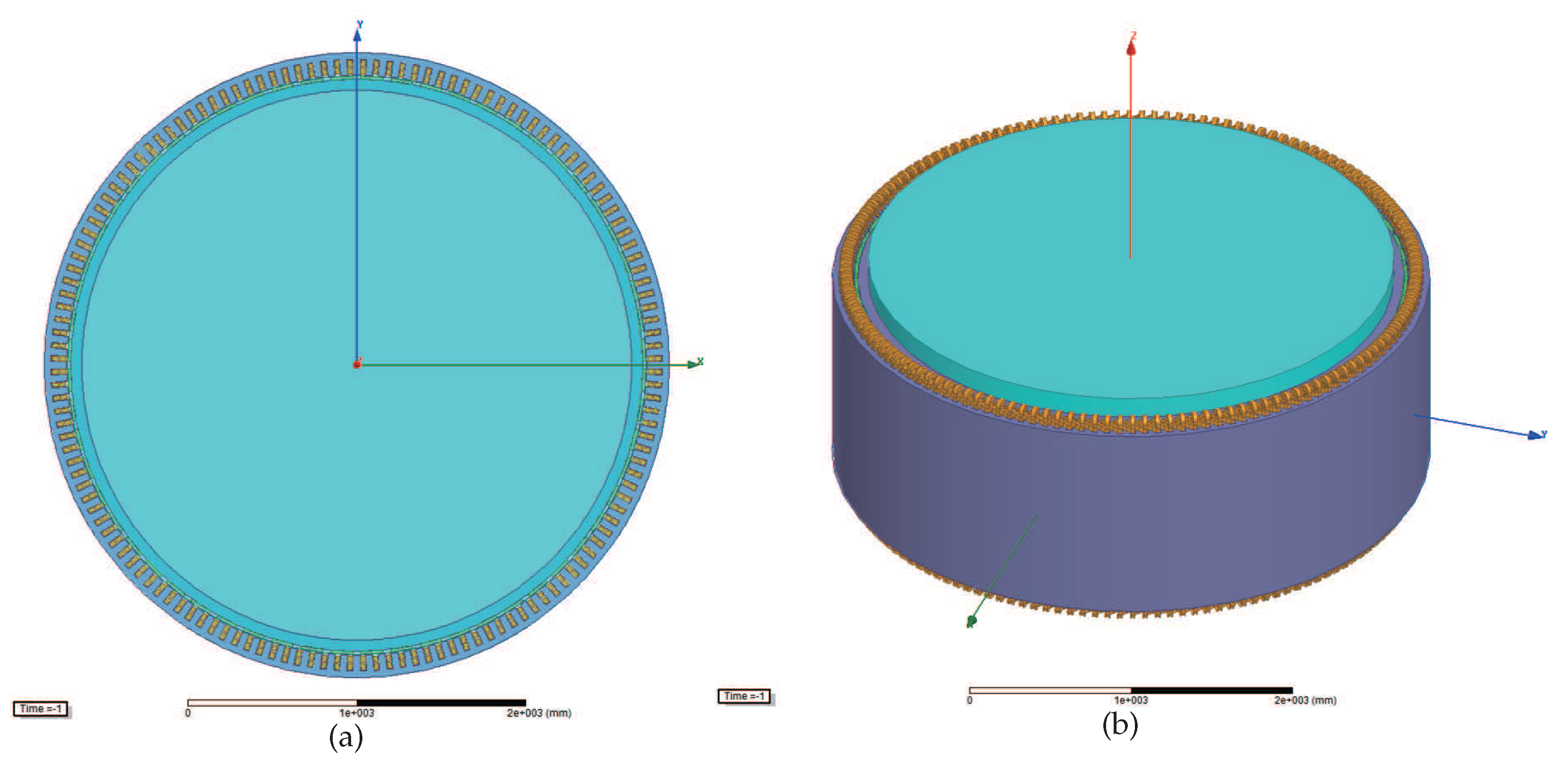
3. Design of 2MW D-SPMSG

To obtain the necessary parameters for analysis, the dynamic behaviors of system (24) and prepare for finite element analysis, a 2 MW D-SPMSG 2D/3D model is designed by ANSYS software according to the practical design requirements. The rated parameters and main dimensions are listed in Table 2. The 2 MW D-SPMSG 2D/3D model is shown in Figure 2.
Then, the necessary system parameters that we need can be obtained, as listed in Table 3. Thus, by calculating Equations (19) and (20) we can get μ = 0 . 6 , ϑ = 6 . 3776 . Below, we will analyze the basic dynamic behaviors of system (24).

4. Basic Dynamic Behavior Analysis

To determine an optimum value of the magnetic flux linkage ψ f in the generator design with a novel design concept by using nonlinear dynamics theory, with ψ f varying, the dynamical behaviors of system (24) are further investigated by equilibrium point, Lyapunov spectrum, bifurcation diagram, phase portrait, and so on.

4.1. Dissipativity and Attractor Existence

The dissipativity of the system (24) is obtained by
V = i ˙ q i q + i ˙ d i d + ω ˙ ω = - 1 - 1 - 2 3 ϑ .
Obviously, from Equation (20) we can get ϑ > 0 , thus, V < 0 . Therefore, the system (24) is a dissipative system with an exponential rate of contraction as:
d V d t = e - 2 - 2 ϑ / 3 .
This means that initial volume V ( 0 ) will shrink to V ( 0 ) e ( - 2 - 2 ϑ / 3 ) t at time t, and when t , volume element V ( 0 ) shrinks to zero. Therefore, all trajectories of the system will be confined to a subset whose volume is zero. In addition, the movement behaviors are gradually fixed in an attractor.

4.2. Equilibrium and Stability

The equilibrium point of system (24) can be found by solving the following equations:
- i q - μ ω i d - μ ψ f ω = 0 , - i d + μ ω i q = 0 , - ϑ ( μ ψ f i q + 2 3 ω ) = 0 .
By calculating, we can easily get three equilibrium points of system (24), as below
P 1 ( 0 , 0 , 0 ) P 2 6 ψ f 2 μ 2 - 4 3 ψ f μ 2 , 2 3 ψ f μ 2 - ψ f , - 6 ψ f 2 μ 2 - 4 2 μ P 3 - 6 ψ f 2 μ 2 - 4 3 ψ f μ 2 , 2 3 ψ f μ 2 - ψ f , 6 ψ f 2 μ 2 - 4 2 μ .
The corresponding Jacobian matrix of system (24) at the equilibrium point P i ( x i , 0 , y i , 0 , z i , 0 ) , i = 1 , 2 , 3 , is depicted by
J = - 1 - μ z i , 0 - μ ( ψ f + y i , 0 ) μ z i , 0 - 1 μ x i , 0 - μ ϑ ψ f 0 - 2 3 ϑ .
Then, the characteristic equation is given as
f ( λ ) = λ 3 + ( 2 3 ϑ + 2 ) λ 2 + ( - ϑ ψ f 2 μ 2 - ϑ ψ f μ 2 y i , 0 + μ 2 z i , 0 2 + 4 3 ϑ + 1 ) λ + 2 3 ϑ - ψ f 2 μ 2 ϑ + 2 3 μ 2 ϑ z i , 0 2 - ϑ ψ f μ 2 y i , 0 - ψ f μ 3 ϑ x i , 0 z i , 0 .
Because the parameters μ, ϑ and ψ f in system (24) are all positive, the range of magnetic flux linkage ψ f can be derived from (30) and (33).
  • For equilibrium point P 1 , the characteristic equation is
    f ( λ ) = λ 3 + ( 2 3 ϑ + 2 ) λ 2 + ( - ϑ ψ f 2 μ 2 + 4 3 ϑ + 1 ) λ + 2 3 ϑ - ϑ ψ f 2 μ 2 .
    If the system is stable at the equilibrium point P 1 , then the real parts of all the roots must be negative. According to the Routh–Hurwitz criterion, system (24) must satisfy the following conditions:
    2 3 ϑ + 2 > 0 - ϑ ψ f 2 μ 2 + 4 3 ϑ + 1 > 0 2 3 ϑ - ϑ ψ f 2 μ 2 > 0 ( 2 3 ϑ + 2 ) ( - ϑ ψ f 2 μ 2 + 4 3 ϑ + 1 ) - ( 2 3 ϑ - ϑ ψ f 2 μ 2 ) > 0 .
    Then, we can get
    0 < ψ f < 2 3 1 μ .
    Thus, 0 < ψ f < 1 . 3608 .
  • For equilibrium points P 2 and P 3 , the characteristic equation is
    f ( λ ) = λ 3 + ( 2 3 ϑ + 2 ) λ 2 + ( 3 2 ψ f 2 μ 2 + 2 3 ϑ ) λ + 2 ϑ ψ f 2 μ 2 - 4 3 ϑ .
    If the system is stable at the equilibrium points P 2 and P 3 , then the real parts of all the roots must be negative. According to the Routh–Hurwitz criterion, system (24) must satisfy the following conditions:
    2 3 ϑ + 2 > 0 3 2 ψ f 2 μ 2 + 2 3 ϑ > 0 2 ϑ ψ f 2 μ 2 - 4 3 ϑ > 0 ( 2 3 ϑ + 2 ) ( 3 2 ψ f 2 μ 2 + 2 3 ϑ ) - ( 2 ϑ ψ f 2 μ 2 - 4 3 ϑ ) > 0 .
    Then, we can get
    • If 0 < ϑ 3 ,
      ψ f > 2 3 1 μ .
      Thus, ψ f > 1 . 3608 .
    • If ϑ > 3 ,
      2 3 1 μ < ψ f < 2 3 μ ϑ ( ϑ + 6 ) ϑ - 3 .
      Thus, 1 . 3608 < ψ f < 5 . 3716 .

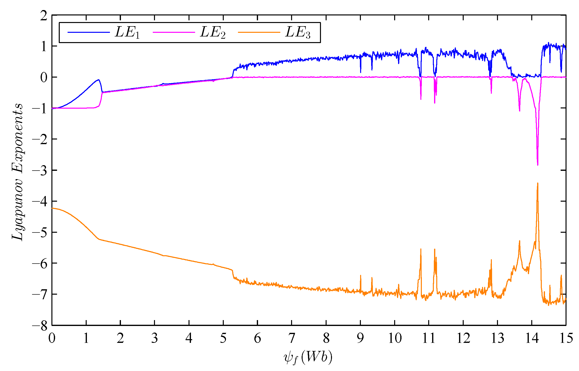
4.3. Lyapunov Exponent Spectrums by Varying Parameters
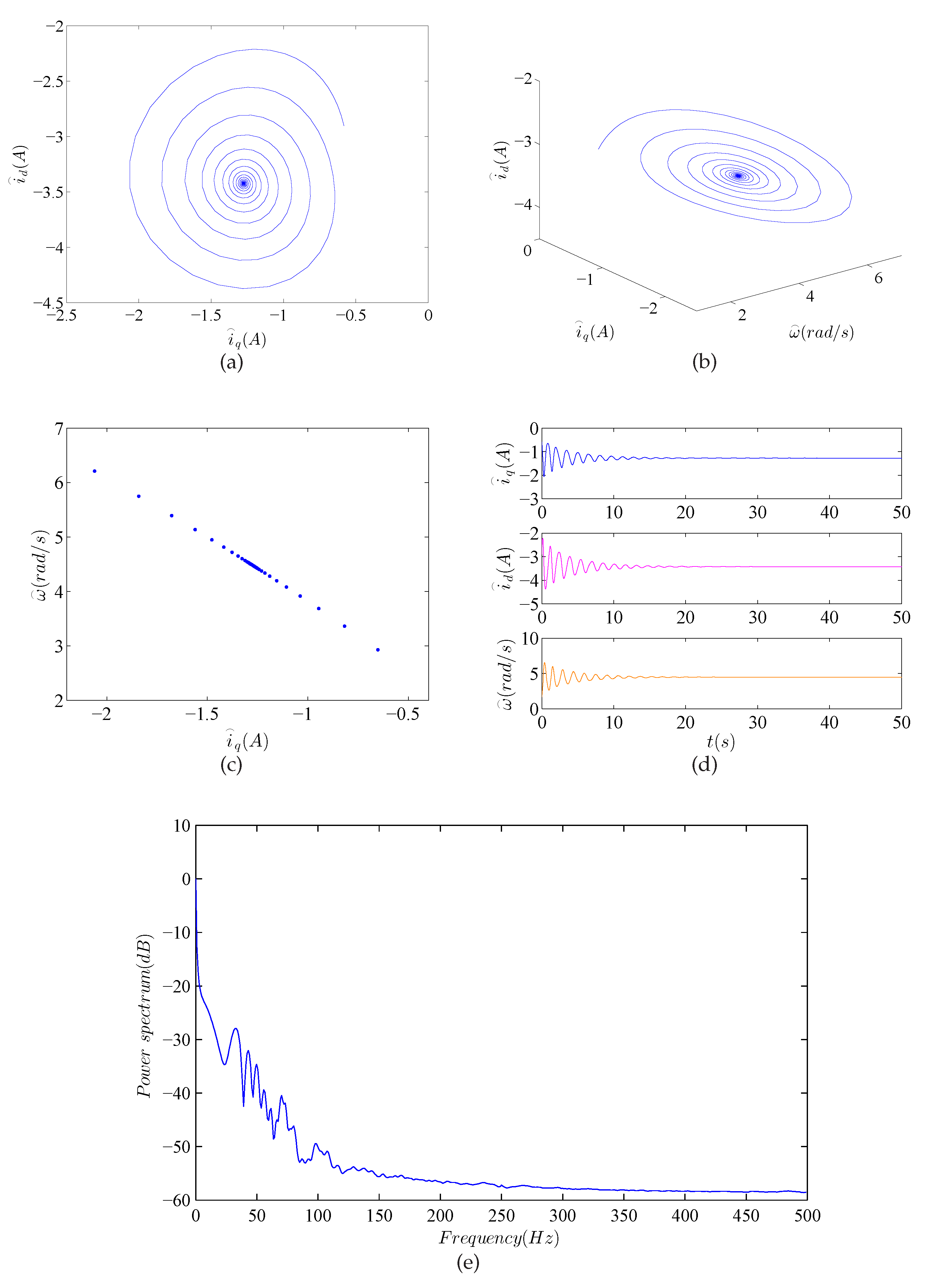
 ψ f

According to Section 3, the basic parameters data of 2MW D-SPMSG are obtained from generator design; thereby, we obtain μ = 0 . 6 , ϑ = 6 . 3776 . Let parameters ψ f vary in some range, and the Lyapunov exponent spectrum of the system (24) with respect to magnetic flux linkage ψ f is displayed in Figure 3. It indicates that the three Lyapunov exponents L E 1 , L E 2 , L E 3 are varying with parameters ψ f respectively, and thus the dynamical behaviors of the system (24) have complex changes along with the parameters ψ f . The stability of the system (24) is summarized as follows:
  • When ψ f ( 0 , 5 . 32 ) , we can obtain L E 1 < 0 , L E 2 < 0 and L E 3 < 0 . For instance, Figure 4 shows phase orbits, Poincaré map, time waveform and power spectrum with ψ f = 3 . 9 , and the Lyapunov exponents are L E 1 = - 0 . 1686 , L E 2 = - 0 . 1964 and L E 3 = - 5 . 8869 . The system is stable with respect to the equilibrium point ( - 1 . 28 , - 3 . 43 , 4 . 48 ) , thus i q , i d and ω tends to be a constant. Furthermore, there are some linear points in the Poincaré map. A regular circle appeared in the phase orbit. Therefore, all of these results indicate that the system can better cope with disturbances and keep steady at this range of the magnetic flux linkage ψ f .
  • When ψ f [ 10 . 75 , 10 . 77 ] [ 11 . 15 , 11 . 18 ) ( 13 . 64 , 13 . 71 ] ( 13 . 83 , 14 . 27 ) , we can obtain L E 1 = 0 , L E 2 < 0 and L E 3 < 0 . For instance, the system dynamical behaviors at ψ f = 14 . 2 are shown in Figure 5, L E 1 = 0 , L E 2 = - 1 . 5957 and L E 3 = - 4 . 6626 . The motion regularities of i q , i d and ω are periodical. A limit cycle appeared in the phase orbit and only some isolated points turn up in the Poincaré map. All of these results indicate that the D-SPMSG system exhibits a periodic vibration and further reveal that the system cannot tend to be stable.
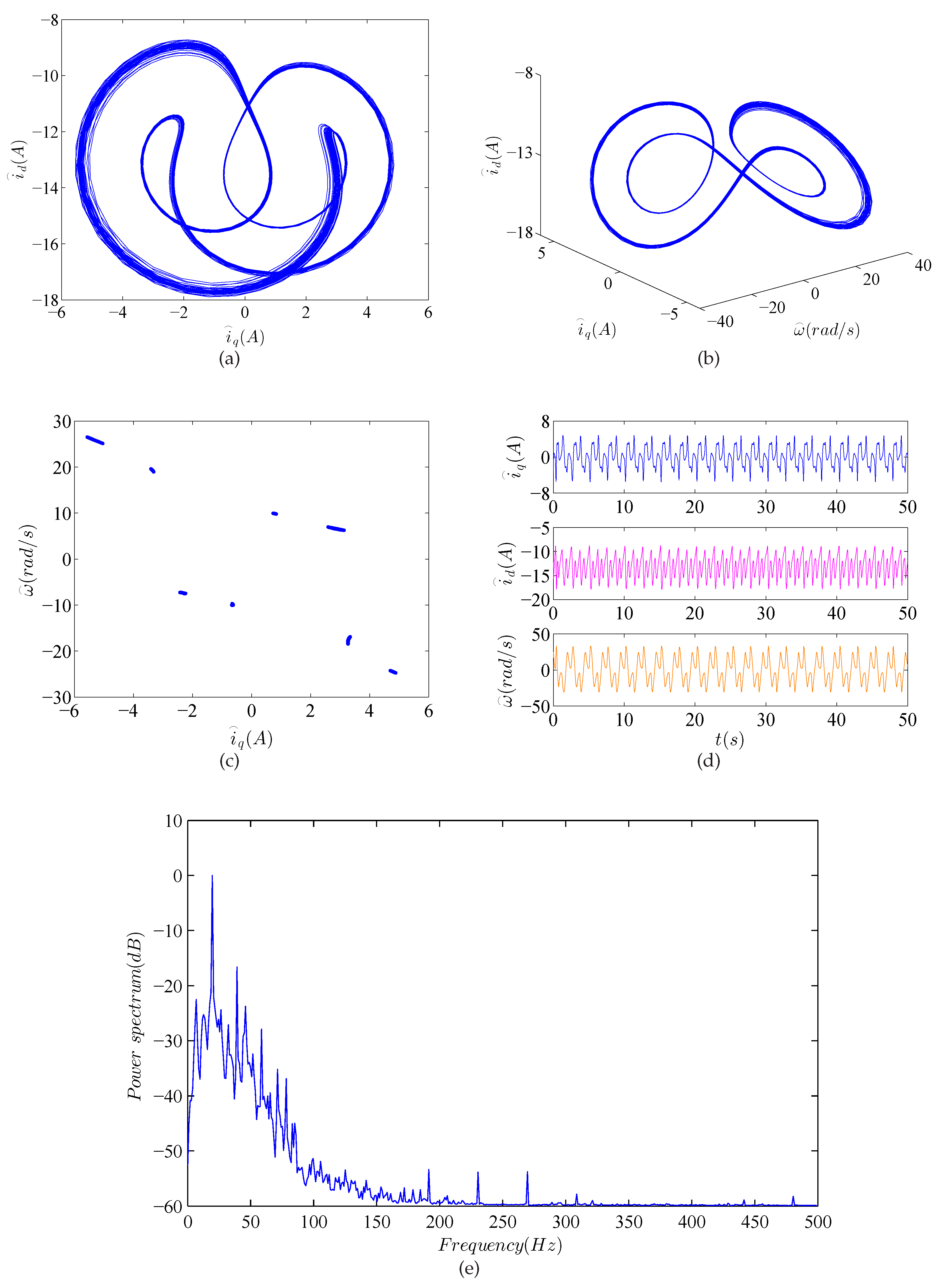
  • When ψ f [ 10 . 73 , 10 . 75 ) ( 12 . 76 , 12 . 79 ] [ 13 . 41 , 13 . 64 ] ( 13 . 71 , 13 . 83 ] , we can obtain L E 1 = 0 , L E 2 = 0 and L E 3 < 0 . For instance, the phase orbits, Poincaré map, time waveform and power spectrum of the system (24) with ψ f = 13 . 44 are depicted in Figure 6, L E 1 = 0 , L E 2 = 0 and L E 3 = - 6 . 3660 . From Figure 6e, the frequency distribution is not as regular as ψ f = 14 . 2 . The system exhibits quasi-periodic motion and results in the two-dimensional torus.
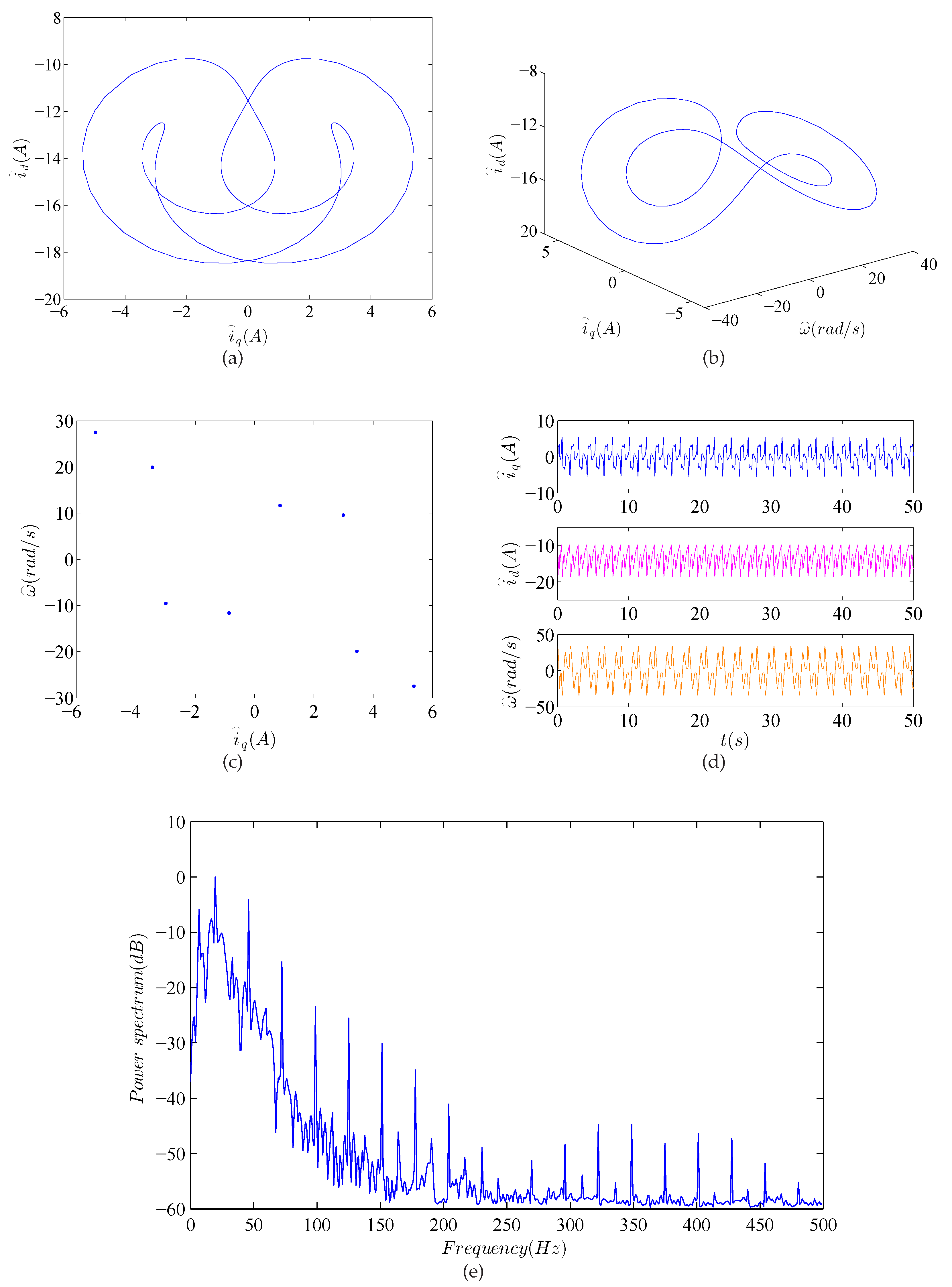
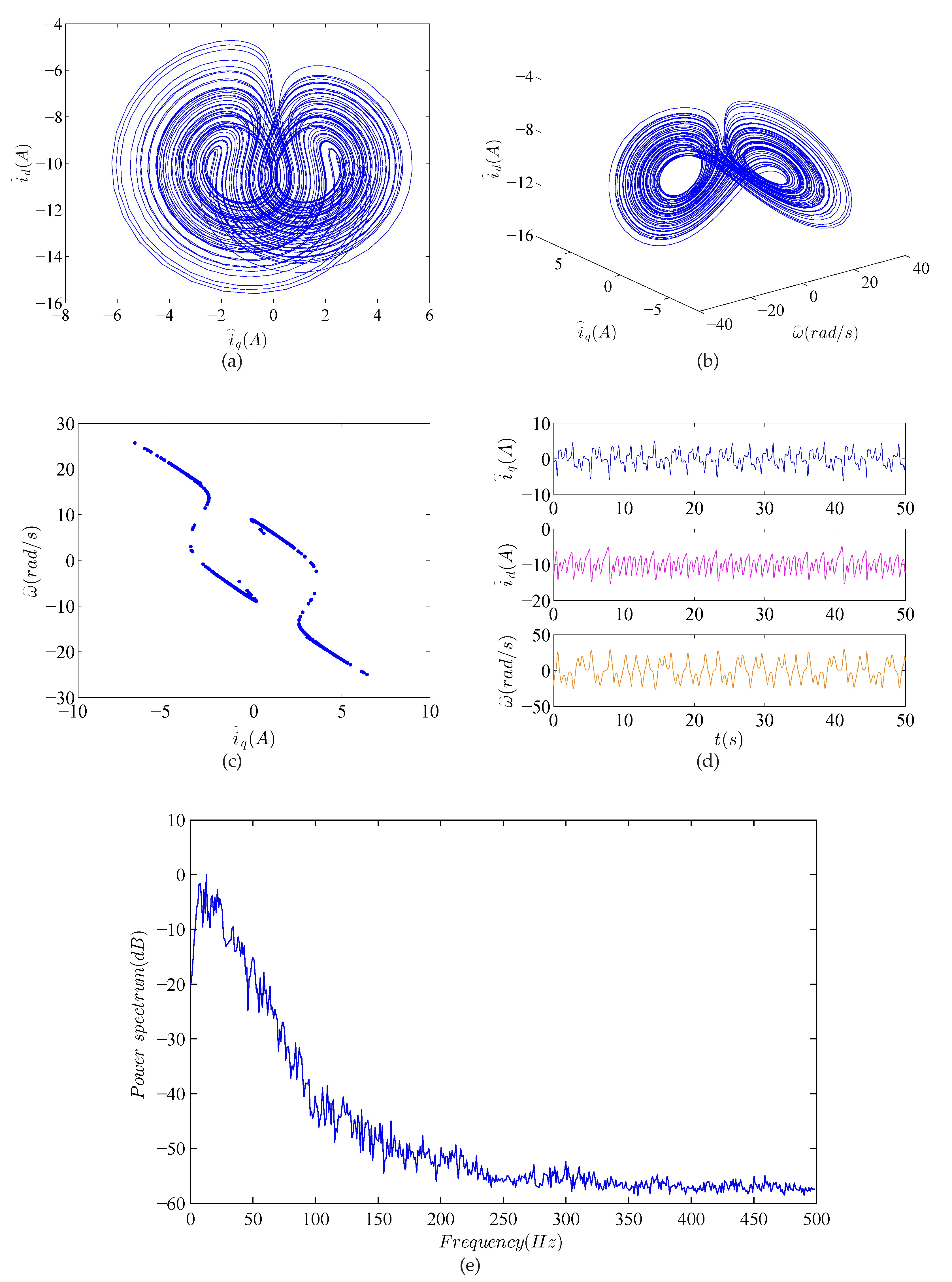
  • When ψ f [ 5 . 32 , 10 . 73 ) ( 10 . 77 , 11 . 15 ) [ 11 . 22 , 12 . 76 ] ) [ 12 . 84 , 13 . 41 ) [ 14 . 27 , 15 ] , we can obtain L E 1 > 0 , L E 2 = 0 and L E 3 < 0 . For instance, the system dynamical behaviors for ψ f = 10 . 5 of the system (24) are depicted in Figure 7, L E 1 = 0 . 8357 , L E 2 = 0 and L E 3 = - 7 . 0830 . The Poincaré map shows patches of dense points, there is a hierarchy dense point, and it has a hierarchical structure. Figure 7e shows a broadband noise-like power spectrum. Therefore, all these results indicate that the system exhibits chaotic motion and results in the chaotic attractor.
Therefore, according to the Lyapunov exponent spectrum in Figure 3, Figure 4, Figure 5, Figure 6 and Figure 7 with ψ f = 3 . 9 , 14 . 2 , 13 . 44 , 10 . 5 show a variety of dynamic behavior characteristics of the four conditions in this section. The numerical simulation results indicate that the point ψ f = 5 . 32 is a critical point, and the D-SPMSG system is steady in the range of 0 < ψ f < 5 . 32 . Thus, the system is unstable while ψ f exceeds 5.32.

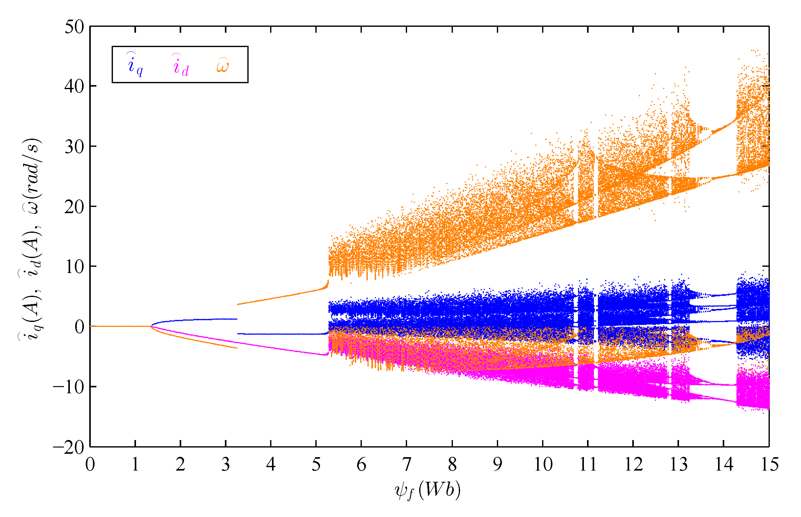
4.4. Bifurcation Diagram by Varying Parameters ψ f

The bifurcation map is used to analyze the dynamical characteristics of the nonlinear system as the system parameter varies. Bifurcation is the main route to chaos from a stable state. The corresponding bifurcation diagram by plotting the maxima of the coordinate i q , i d and ω with parameter ψ f varying is as shown in Figure 8. It is clear that the bifurcation diagram coincides well with the Lyapunov exponents spectrum. From Figure 8, the point ψ f = 5 . 32 is a critical point, which is the one of the occurrence of bifurcation. Apparently, as the magnetic flux linkage ψ f changes, the running state of the system changes accordingly, which demonstrates that the system is unstable while ψ f exceeds the critical value.

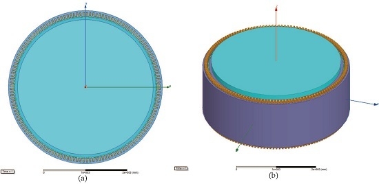
5. Finite Element Analysis of D-SPMSG

According to the above discussion and analysis, a new kind of magnetic flux linkage optimization method is proposed. First, in order to facilitate the design and dynamic analysis, a new compact representation of the D-SPMSG equations is obtained in this method, and it is discussed in Section 2.2. Second, for the sake of having an optimum value of magnetic flux linkage, the nonlinear dynamic analysis about D-SPMSG with respect to magnetic flux linkage is discussed as described in Section 4. From the Lyapunov exponent spectrum in Figure 3 and the bifurcation diagram in Figure 8, we can know that the system is increasingly unstable, as ψ f is increasing, but for the range 0 < ψ f < 5 . 32 , the system is obviously steady. Third, in order to further determine an optimum value of magnetic flux linkage, the finite element analysis (FEA) of the D-SPMSG model mentioned in Section 3 will be studied in detail in this section, and also demonstrates the effectiveness of this method.
It is known that one representative method to optimize magnetic flux linkage is adjusting the size of the permanent magnet. Accordingly, if the value of the magnetic flux linkage is too small, magnetic flux density will be reduced, which will affect the performance of D-SPMSG to reach the operational requirements, and if the value of the magnetic flux linkage is too large, magnetic flux density will be saturated, and this will cause unstable operation, overheating and unit vibration of D-SPMSG. Therefore, in order for the generator to optimize performances, the value of the magnetic flux linkage is chosen as close as possible to the right open interval in the range 0 < ψ f < 5 . 32 . Then, based on the finite element analysis (FEA) method and by using the electromagnetic field analysis software ANSYS Maxwell (Version 14.5), five cases of D-SPMSG model in Section 3 with different magnetic flux linkage are simulated, respectively.
Remark 2. 
According to practical engineering experience, when the magnetic flux density is nearing saturation ( B 1 . 6 T), the generator will achieve the optimal efficiency and performance.
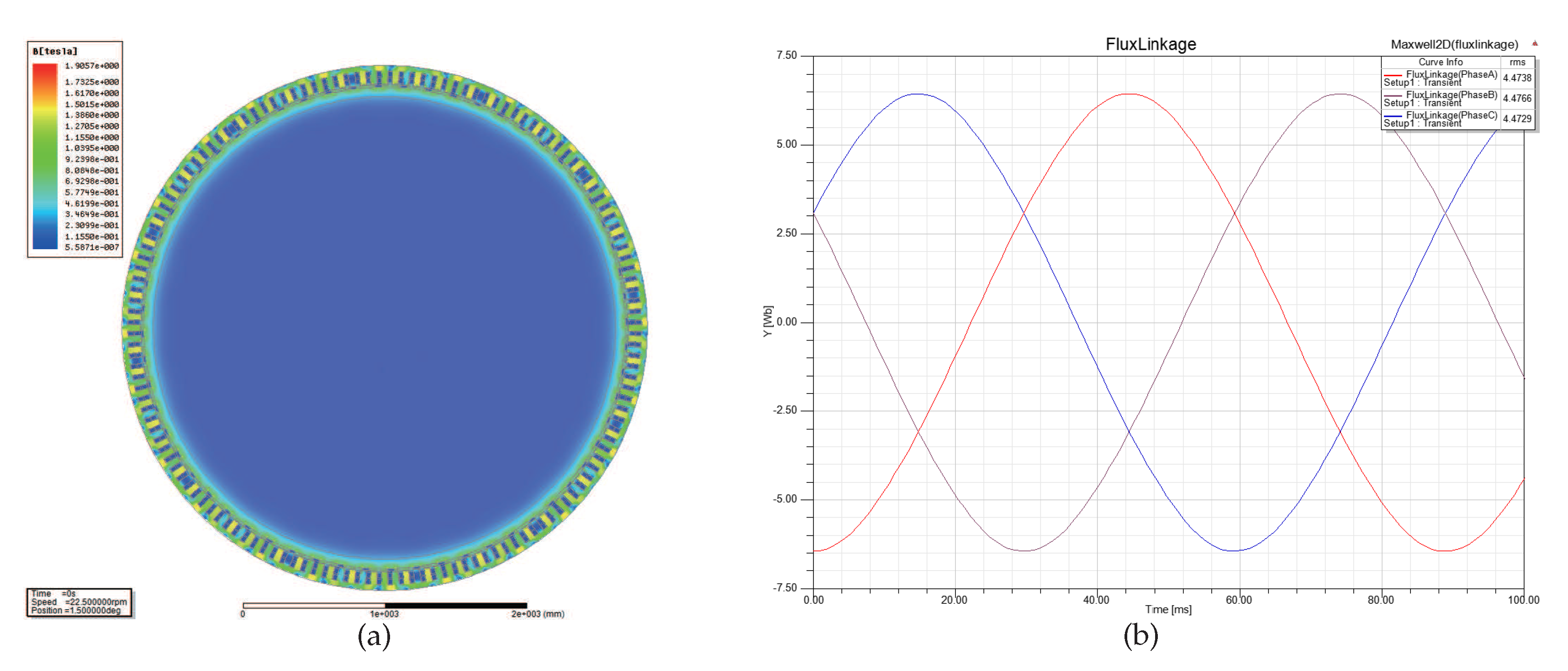
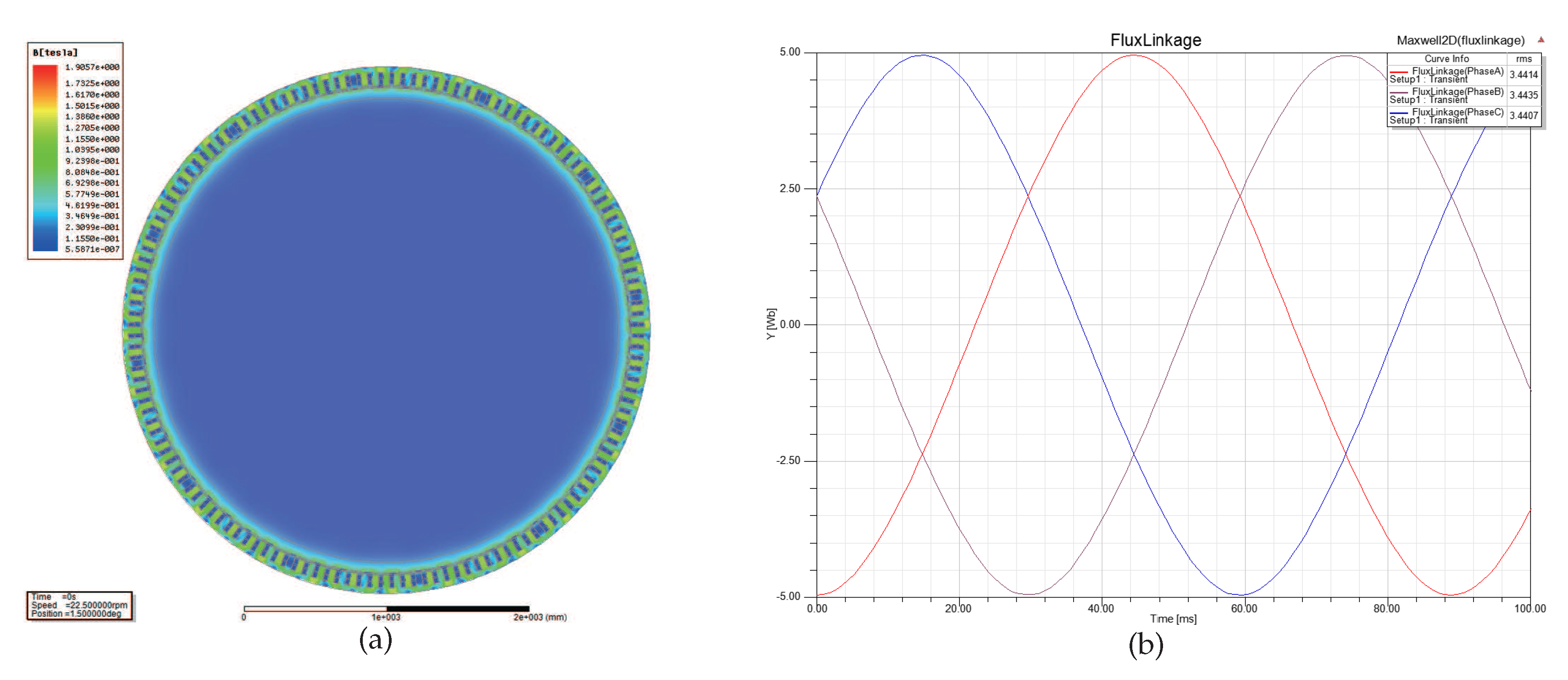
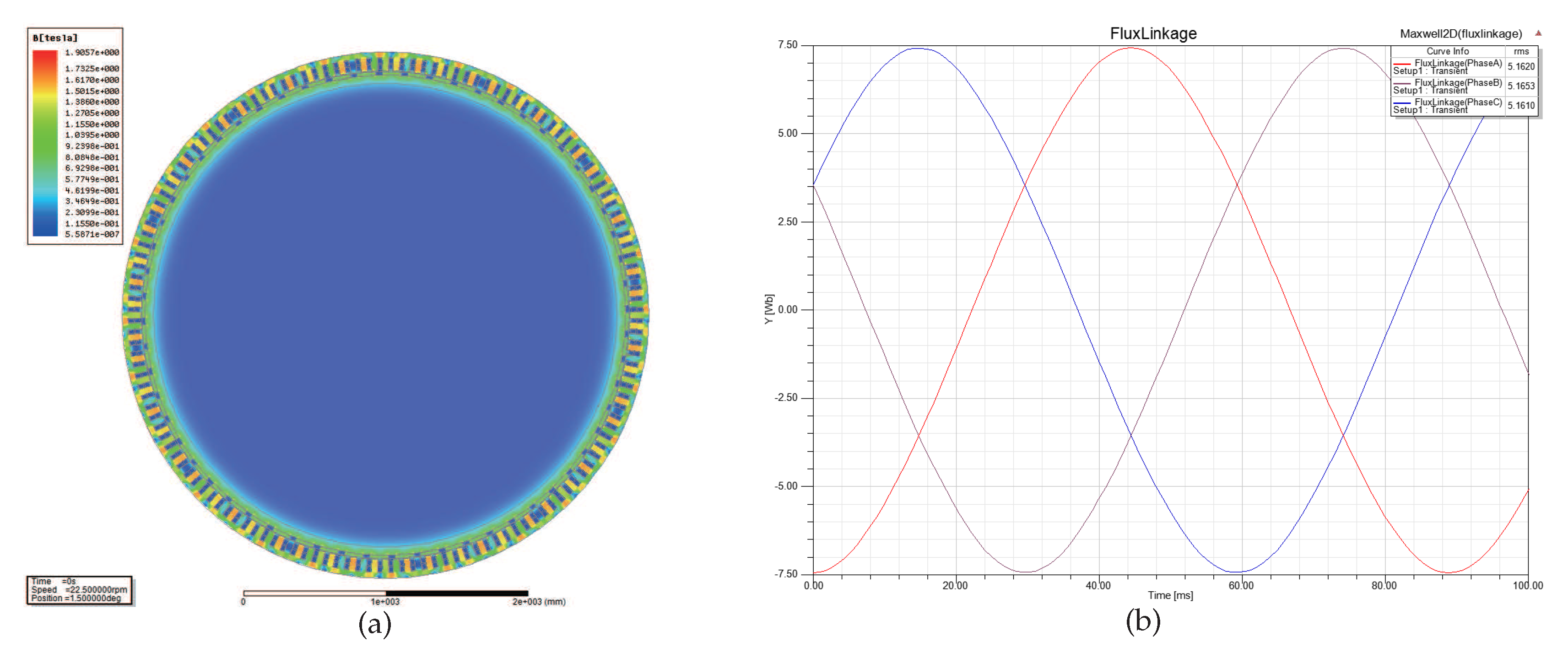
  • Case 1 and Case 2: Figure 9 and Figure 10 show the nephogram of magnetic flux density and the corresponding waveform of magnetic flux linkage with ψ f 3 . 44 Wb and ψ f 4 . 47 Wb, respectively. We can observe the magnetic flux density B 1.2 T in Figure 9 and B 1 . 4 T in Figure 10. Thus, this indicates that the performance of D-SPMSG is improving, as ψ f is increasing. However, low utilization ratio of generator material in these two cases results in a waste of permanent magnet material.
  • Case 3: The nephogram of magnetic flux density and the waveform of magnetic flux linkage at ψ f 5 . 16 Wb are shown in Figure 11. It is obviously B 1.6 T; in other words, the magnetic flux density is nearing saturation. In this case, the saturation point of magnetic flux density at each stator-teeth and stator-yoke are discontinuous, that is to say, permanent magnets work at the optimal operating point, thus maximizing the utilization ratio of generator material and optimizing the performances.
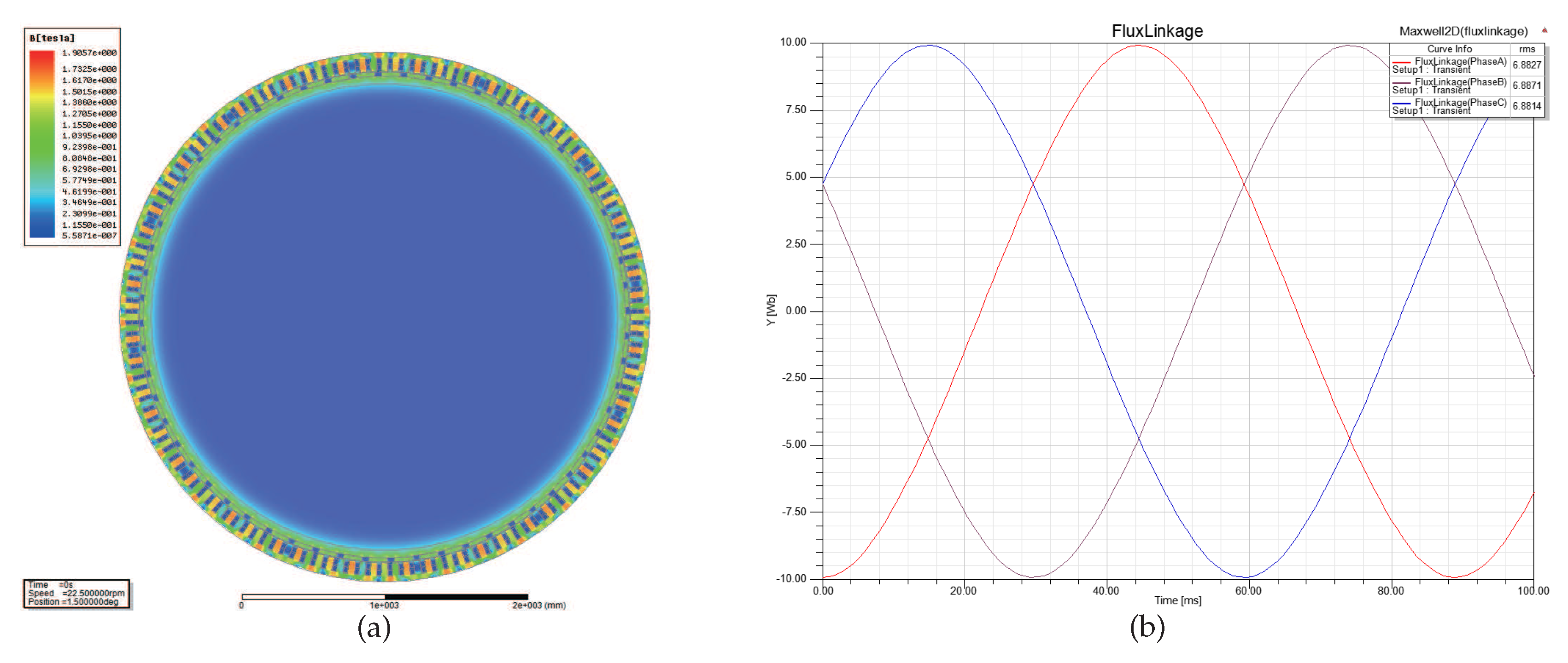
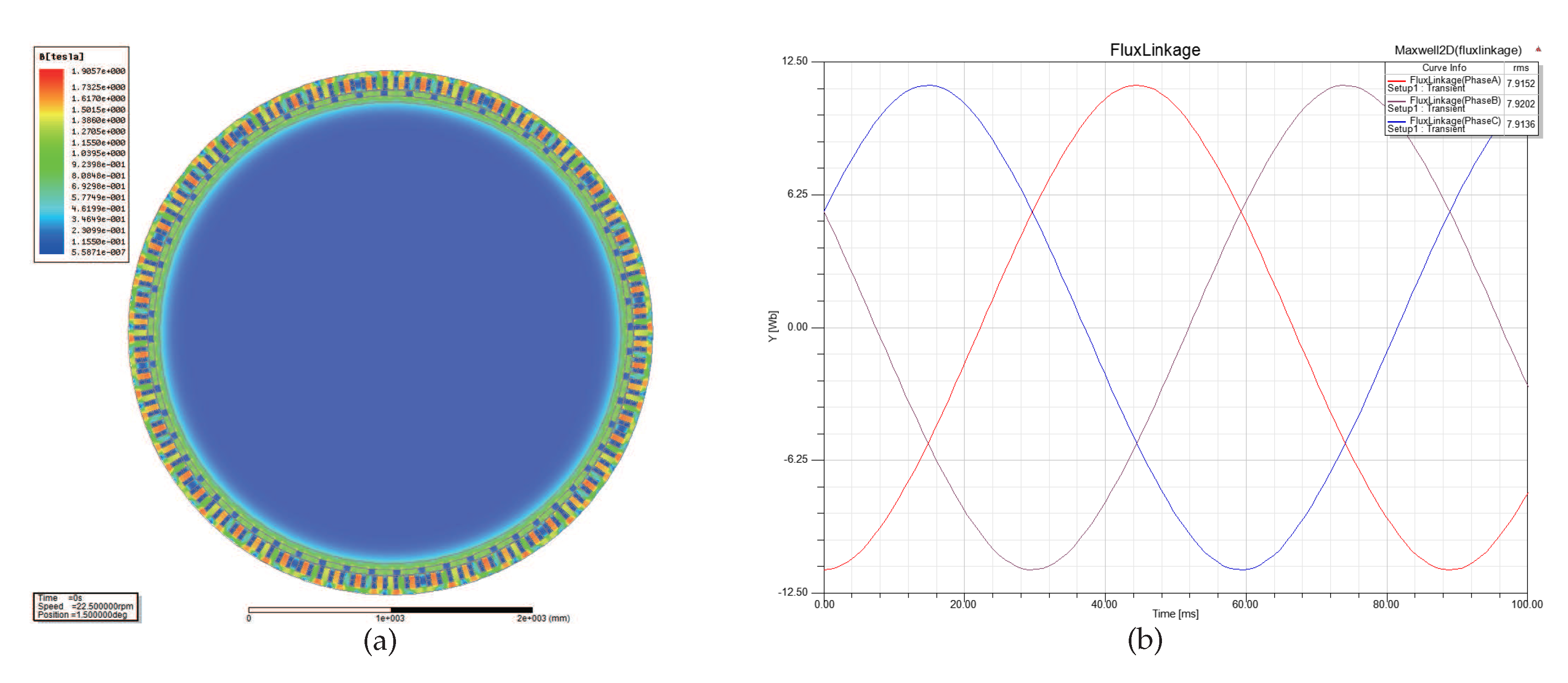
  • Case 4 and Case 5: For ψ f 6.88 Wb and ψ f 7.92 Wb, the nephogram of magnetic flux density and the corresponding waveform of magnetic flux linkage are shown in Figure 12 and Figure 13. Hence, the magnetic flux density B 1.75 T and B 1.9 T are obtained in Figure 12 and Figure 13 respectively. It is obvious that the saturation points of magnetic flux density at each stator-teeth and stator-yoke are continuous. Therefore, this implies that the D-SPMSG is increasingly unstable as ψ f is increasing. In these two cases, the excessive magnetic flux density will cause the generator to have unstable operation, overheating , unit vibration, speed fluctuation, output voltage instability and other problems.
The corresponding permanent magnet specifications and dimensions in the optimal Case 3, namely ψ f 5.16 Wb, are shown in Table 4. The winding arrangements are shown in Table 5.
Therefore, the magnetic flux linkage optimization of D-SPMSG should not only consider the conventional optimization of power efficiency and empirical formula, but also needs to avoid the occurrence of unstable states based on the newly compact system Equation (24).

6. Conclusions

In this paper, we propose a novel method for magnetic flux linkage optimization of D-SPMSG based on a nonlinear dynamic theory. The method is through the use of the affine transformation to establish a compact representation of the D-SPMSG nonlinear dynamic differential equations, and the number of system parameters has been greatly reduced. Then, according to the practical design requirements, a 2D/3D model of 2MW D-SPMSG is designed. Subsequently, the nonlinear dynamical behaviors of the D-SPMSG system in the process of magnetic flux linkage variations are presented including dissipativity, equilibrium point and stability, Lyapunov exponent spectrums, phase orbits, Poincaré maps, time waveforms and bifurcation diagrams. The numerical simulation results indicate that the D-SPMSG system is steady in the range of 0 < ψ f < 5 . 32 . Eventually, considering the generator for optimum performance, the value of the magnetic flux linkage is chosen as close as possible to the right open interval in the stable range. Five cases of D-SPMSG models with different magnetic flux linkages are simulated by using the finite element analysis (FEA) method, and all of the results demonstrate the correctness and effectiveness of the proposed approach.

Acknowledgments

This work is supported by the National Science Foundation for Post-Doctoral Scientists of China (Grant No. 2013M530426), the National Science Foundation for Young Scientists of China (Grant No. 51507134), and the Scientific Research Program Funded by Shaanxi Provincial Education Department (Grant No. 5JK1537).

Author Contributions

Qian Xie conceived and developed the main parts of the research work which includes system modelling, nonlinear dynamics simulation, and analyses of the results obtained; Yanan Yu contributed in generator design; Ningning Yang and Longfei Luo were in charged in verifying the work; Yanbin Zhang and Gangquan Si were provided the guidance and supervision; and Qian Xie wrote the paper.

Conflicts of Interest

The authors declare no conflict of interest.

References

  1. Haque, M.E.; Negnevitsky, M.; Muttaqi, K.M. A Novel Control Strategy for a Variable-Speed Wind Turbine with a Permanent-Magnet Synchronous Generator. IEEE Trans. Ind. Appl. 2010, 46, 331–339. [Google Scholar] [CrossRef]
  2. Yun-Su, K.; Il-Yop, C.; Seung-Il, M. Tuning of the PI Controller Parameters of a PMSG Wind Turbine to Improve Control Performance under Various Wind Speeds. Energies 2015, 8, 1406–1425. [Google Scholar]
  3. Bhende, C.N.; Mishra, S.; Malla, S.G. Permanent Magnet Synchronous Generator-Based Standalone Wind Energy Supply System. IEEE Trans. Sustain. Energy 2011, 2, 361–373. [Google Scholar] [CrossRef]
  4. Hui, H.; Chengxiong, M.; Jiming, L.; Dan, W. Electronic Power Transformer Control Strategy in Wind Energy Conversion Systems for Low Voltage Ride-through Capability Enhancement of Directly Driven Wind Turbines with Permanent Magnet Synchronous Generators (D-PMSGs). Energies 2014, 7, 7330–7347. [Google Scholar]
  5. Liu, K.; Zhu, Z.Q. Online Estimation of the Rotor Flux Linkage and Voltage-Source Inverter Nonlinearity in Permanent Magnet Synchronous Machine Drives. IEEE Trans. Power Electron. 2014, 29, 418–427. [Google Scholar] [CrossRef]
  6. Zaijun, W.; Xiaobo, D.; Jiawei, C.; Minqiang, H. Operation and Control of a Direct-Driven PMSG-Based Wind Turbine System with an Auxiliary Parallel Grid-Side Converter. Energies 2013, 6, 3405–3421. [Google Scholar]
  7. Arumugam, P.; Hamiti, T.; Brunson, C.; Gerada, C. Analysis of Vertical Strip Wound Fault-Tolerant Permanent Magnet Synchronous Machines. IEEE Trans. Ind. Electron. 2014, 61, 1158–1168. [Google Scholar] [CrossRef]
  8. Tang, Y.; Xing, X.; Karimi, H.R.; Kocarev, L.; Kurths, J. Tracking Control of Networked Multi-Agent Systems Under New Characterizations of Impulses and Its Applications in Robotic Systems. IEEE Trans. Ind. Electron. 2016, 63, 1299–1307. [Google Scholar] [CrossRef]
  9. Coria, L.N.; Starkov, K.E. Bounding a domain containing all compact invariant sets of the permanent-magnet motor system. Commun. Nonlinear Sci. Numer. Simul. 2009, 14, 3879–3888. [Google Scholar] [CrossRef]
  10. Tang, Y.; Gao, H.J.; Zhang, W.B.; Kurths, J. Leader-following consensus of a class of stochastic delayed multi-agent systems with partial mixed impulses. Automatica 2015, 53, 346–354. [Google Scholar] [CrossRef]
  11. Yu, J.P.; Yu, H.S.; Chen, B.; Gao, J.W.; Qin, Y. Direct adaptive neural control of chaos in the permanent magnet synchronous motor. Nonlinear Dyn. 2012, 70, 1879–1887. [Google Scholar] [CrossRef]
  12. Xie, Q.; Si, G.Q.; Zhang, Y.B.; Yuan, Y.W.; Yao, R. Finite-time synchronization and identification of complex delayed networks with Markovian jumping parameters and stochastic perturbations. Chaos Solitons Fractals 2016, 86, 35–49. [Google Scholar] [CrossRef]
  13. Rasoolzadeh, A.; Tavazoei, M.S. Prediction of chaos in non-salient permanent-magnet synchronous machines. Phys. Lett. A 2012, 377, 73–79. [Google Scholar] [CrossRef]
  14. Wu, X.T.; Tang, Y.; Zhang, W.B. Input-to-state stability of impulsive stochastic delayed systems under linear assumptions. Automatica 2016, 66, 195–204. [Google Scholar] [CrossRef]
  15. Jing, Z.J.; Yu, C.; Chen, G.R. Complex dynamics in a permanent-magnet synchronous motor model. Chaos Solitons Fractals 2004, 22, 831–848. [Google Scholar] [CrossRef]
  16. Tang, Y.; Wang, Z.D.; Gao, H.J.; Qiao, H.; Kurths, J. On Controllability of Neuronal Networks with Constraints on the Average of Control Gains. IEEE Trans. Cybern. 2014, 44, 2670–2681. [Google Scholar] [CrossRef] [PubMed]
  17. Lu, P.L.; Yang, Y.; Huang, L. Global Dynamic Properties of a Synchronous Machine Model. Int. J. Bifurc. Chaos 2008, 18, 3113–3128. [Google Scholar] [CrossRef]
  18. Li, Z.; Park, J.B.; Joo, Y.H.; Zhang, B.; Chen, G.R. Bifurcations and chaos in a permanent-magnet synchronous motor. IEEE Trans. Circuits Syst. I-Fundam. Theory Appl. 2002, 49, 383–387. [Google Scholar]
  19. Hemati, N. Strange Attractors in Brushless DC Motors. IEEE Trans. Circuits Syst. I-Fundam. Theory Appl. 1994, 41, 40–45. [Google Scholar] [CrossRef]
  20. Chen, D.Y.; Liu, S.; Ma, X.Y. Modeling, nonlinear dynamical analysis of a novel power system with random wind power and it’s control. Energy 2013, 53, 139–146. [Google Scholar] [CrossRef]
  21. Slemon, G.R. On the Design of High-Performance Surface-Mounted PM Motors. IEEE Trans. Ind. Appl. 1994, 30, 134–140. [Google Scholar] [CrossRef]
  22. Gao, Y.; Chau, K.T. Design of permanent magnets to avoid chaos in doubly salient PM machines. IEEE Trans. Magn. 2004, 40, 3048–3050. [Google Scholar] [CrossRef]
  23. Romeral, L.; Urresty, J.C.; Ruiz, J.R.R.; Espinosa, A.G. Modeling of Surface-Mounted Permanent Magnet Synchronous Motors with Stator Winding Interturn Faults. IEEE Trans. Ind. Electron. 2011, 58, 1576–1585. [Google Scholar] [CrossRef]
  24. Silva, R.; Salimi, A.; Li, M.; Freitas, A.R.R.; Guimaraes, F.G.; Lowther, D.A. Visualization and Analysis of Tradeoffs in Many-Objective Optimization: A Case Study on the Interior Permanent Magnet Motor Design. IEEE Trans. Magn. 2016, 52. [Google Scholar] [CrossRef]
  25. Yang, L.; Ho, S.L.; Fu, W.N.; Li, W. Design Optimization of a Permanent Magnet Motor Derived from a General Magnetization Pattern. IEEE Trans. Magn. 2015, 51. [Google Scholar] [CrossRef]
  26. Virtic, P.; Vrazic, M.; Papa, G. Design of an Axial Flux Permanent Magnet Synchronous Machine Using Analytical Method and Evolutionary Optimization. IEEE Trans. Energy Convers. 2016, 31, 150–158. [Google Scholar] [CrossRef]
Figure 1. A diagram of the space vector of direct-driven surface-mounted permanent magnet synchronous generator (D-SPMSG).
Energies 09 00557 g001
Figure 2. 2 MW D-SPMSG design model: (a) 2D-model of D-SPMSG; (b) 3D-model of D-SPMSG.
Energies 09 00557 g002
Figure 3. Lyapunov exponent spectrum of the D-SPMSG system (24) versus ψ f .
Energies 09 00557 g003
Figure 4. Numerical analysis of nonlinear dynamic behavior with ψ f = 3 . 9 : (a) Phase orbit with i q i d ; (b) Phase orbit with ω i q i d ; (c) Poincaré map; (d) Time waveforms; (e) Power spectrum.
Energies 09 00557 g004
Figure 5. Numerical analysis of nonlinear dynamic behavior with ψ f = 14 . 2 : (a) Phase orbit with i q i d ; (b) Phase orbit with ω i q i d ; (c) Poincaré map; (d) Time waveforms; (e) Power spectrum.
Energies 09 00557 g005
Figure 6. Numerical analysis of nonlinear dynamic behavior with ψ f = 13 . 44 : (a) Phase orbit with i q i d ; (b) Phase orbit with ω i q i d ; (c) Poincaré map; (d) Time waveforms; (e) Power spectrum.
Energies 09 00557 g006
Figure 7. Numerical analysis of nonlinear dynamic behavior with ψ f = 10 . 5 : (a) Phase orbit with i q i d ; (b) Phase orbit with ω i q i d ; (c) Poincaré map; (d) Time waveforms; (e) Power spectrum.
Energies 09 00557 g007
Figure 8. Bifurcation diagram of the D-SPMSG system (24) versus ψ f .
Energies 09 00557 g008
Figure 9. Results of finite element analysis with ψ f 3 . 44 Wb in Case 1: (a) Nephogram of magnetic flux density; (b) Corresponding waveform of magnetic flux linkage.
Energies 09 00557 g009
Figure 10. Results of finite element analysis with ψ f 4 . 47 Wb in Case 2: (a) Nephogram of magnetic flux density; (b) Corresponding waveform of magnetic flux linkage.
Energies 09 00557 g010
Figure 11. Results of finite element analysis with ψ f 5.16 Wb in Case 3: (a) Nephogram of magnetic flux density; (b) Corresponding waveform of magnetic flux linkage.
Energies 09 00557 g011
Figure 12. Results of finite element analysis with ψ f 6 . 88 Wb in Case 4: (a) Nephogram of magnetic flux density; (b) Corresponding waveform of magnetic flux linkage.
Energies 09 00557 g012
Figure 13. Results of finite element analysis with ψ f 7.92 Wb in Case 5: (a) Nephogram of magnetic flux density; (b) Corresponding waveform of magnetic flux linkage.
Energies 09 00557 g013
Table 1. System parameters.
ParametersDescriptionsUnit
RStator winding resistanceΩ
L q q-axis stator inductanceH
L d d-axis stator inductanceH
u q q-axis stator voltageV
u d d-axis stator voltageV
i q q-axis stator currentA
i d d-axis stator currentA
ψ q q-axis stator fluxWb
ψ d d-axis stator fluxWb
ψ f Flux of permanent magnetWb
T w Mechanical torqueN·m
T e Electromagnetic torqueN·m
n p Number of pole pairs-
ωRotor angular speedrad/s
ω e Electrical angular frequencyrad/s
bFriction coefficientN·m · (rad/s) - 1
JMoment of inertiakg · m 2
Table 2. Direct-driven surface-mounted permanent magnet synchronous generator (D-SPMSG) design requirements: rated parameters and main dimensions.
ParametersDescriptionsValues
mNumber of stator phase3
T y p e Type of circuitY
U N Rated voltage660 V
T N Rated torque 8 . 48 × 10 5 N · m
n N Rated speed22.5 rpm
cos φ N Rated power factor0.98
n p Number of pole pairs30
QNumber of stator slots144
fRated frequency11.25 Hz
P N Rated output power2000 KW
η N Rated efficiency95%
D o Outer diameter of stator3750 mm
D i Inner diameter of stator3480 mm
δAir gap5 mm
D o 2 Outer diameter of rotor3470 mm
D i 2 Inner diameter of rotor3300 mm
lLength of rotor1300 mm
Table 3. D-SPMSG data.
ParametersValues
R 10 - 2 Ω
L d 8 × 10 - 4 H
L q 8 × 10 - 4 H
n p 30
b 5 × 10 3 N · m · s/rad
J 14 × 10 4 kg · m 2
Table 4. Permanent magnet specifications and dimensions.
ParametersValues
Residual flux density1.3223 T
Coercive force915 kA/m
Maximum energy density302.475 kJ / m 3
Relative recoil permeability1.15003
Mechanical pole embrace0.72
Length of magnet1300 mm
Outer diameter of magnet3470 mm
Inner diameter of magnet3431.6 mm
Thickness of magnet19.2 mm
Width of magnet130.092 mm
Table 5. Winding arrangement.
ParametersValues
Winding typeThe 3-phase, 2-layer winding
Coil pitch2
Number of wires per conductor2
Wire diameter5.971 mm
Wire wrap thickness0.1 mm

