
A Novel Strategy for Optimising Decentralised Energy Exchange for Prosumers


Johann Bernoulli Institute, University of Groningen, Nijenborgh 9, 9747AG Groningen, The Netherlands
*
Author to whom correspondence should be addressed.
Energies 2016, 9(7), 554; https://doi.org/10.3390/en9070554
Submission received: 30 April 2016
/
Revised: 1 July 2016
/
Accepted: 12 July 2016
/
Published: 18 July 2016
(This article belongs to the Special Issue Decentralized Management of Energy Streams in Smart Grids)
Abstract
:The realization of the Smart Grid vision will change the way of producing and distributing electrical energy. It paves the road for end-users to become pro-active in the distribution system and, equipped with renewable energy generators such as a photovoltaic panel, to become a so called “prosumer”. The prosumer is engaged in both energy production and consumption. Prosumers’ energy can be transmitted and exchanged as a commodity between end-users, disrupting the traditional utility model. The appeal of such scenario lies in the engagement of the end user, in facilitating the introduction and optimization of renewables, and in engaging the end-user in its energy management. To facilitate the transition to a prosumers’ governed grid, we propose a novel strategy for optimizing decentralized energy exchange in digitalized power grids, i.e., the Smart Grid. The strategy considers prosumer’s involvement, energy loss of delivery, network topology, and physical constraints of distribution networks. To evaluate the solution, we build a simulation program and design three meaningful evaluation cases according to different energy flow patterns. The simulation results indicate that, compared to traditional power distribution system, the maximum reduction of energy loss, energy costs, energy provided by the electric utility based using the proposed strategy can reach , , , depending on the strategy. Moreover, the proportion of energy self-satisfaction approaches reaches .
1. Introduction
The traditional way of producing and distributing electrical energy is undergoing major changes. From a hierarchical system where energy is centrally produced and ‘pushed’ down to the users, we currently experience more and more distributed generation with energy flows that become multi-directional. According to the US Department of Energy [1], the Smart Grid is a term used to illustrate the evolution of the Power Grid that adopts Information and Communication Technology (ICT) to improve its efficiency, reliability, economics, and environmental sustainability. Traditional power systems are centralised with respect to energy generation (i.e., thermal and nuclear power generation), energy providers (i.e., electric utility), and operate a hierarchical energy transmission and radial energy distribution networks. Its overall efficiency is about 30% [2]. However, the Smart Grid introduces distributed energy generation (DEG) based on renewable energy sources (RESs) and decentralised energy exchange in distribution networks based on bidirectional flows of energy. Compared to the traditional power system, the Smart Grid with distributed energy generation providers a much higher efficiency that is estimated to approach a value of 70% [2].
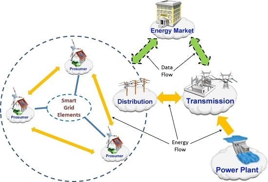
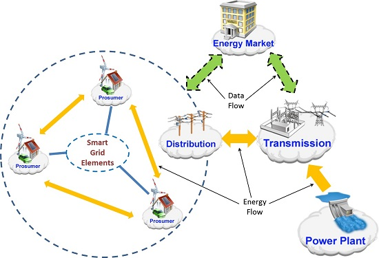
In the present work, we assume a future scenario where renewable energy generators based on photovoltaic (PV) panels and small wind turbines enable end-users to produce electrical energy and to distribute it freely among each other. In other terms, all end-users are connected to local energy markets. After fulfilling their individual needs, their surplus energy can be transmitted to other end-users that need to buy energy. The motivation for the exchange is monetary. This means that there can be multiple energy providers supplying energy at various prices. The end-user engaged in both energy production and consumption is called a prosumer. We use the term decentralised energy exchange to express the trading of surplus energy among prosumers in the distribution network. By contrast, centralised energy exchange is that end-users buy energy from or send their surplus energy to a centralized operator. All of the features described above compose a Prosumer-involved Smart Grid. Achieved by encouraging distributed energy generation and decentralised energy exchange on a local scale (i.e., in the same distribution network), the Prosumer-involved Smart Grid offers two important advantages: reducing the consumption of energy sources based on fossil fuels; and improving independence from the centralised energy generation and central energy providers [1]. In this paper, we consider the medium and low voltage grids as part of the distribution network, including the substations. With the term “local scale” we identify residential area that is covered by a sub-network of the distribution network running at low voltage without substations.
The present paper focuses on optimising decentralised energy exchange in the Prosumer-involved Smart Grid considering prosumer involvement, energy loss of delivery, topologies, energy flows, and physical constraints of the distribution network. The optimisation objectives are to reduce energy loss of delivery, to enhance independence from centralised energy generation and central energy providers, and to decrease energy costs for the end-users. To achieve these goals, we proposed a mathematical model of the optimisation problem and a peer-to-peer (P2P) model of the Prosumer-involved Smart Grid. The models are richer than purely topological ones in considering also basic power flows, while simpler than detailed power flow models. In other terms, one has to find a balance between adequate physical modelling and the scale at which a phenomenon can be observed. Given our interest in looking at possible alternative distribution alternatives, we chose an intermediate approach between a traditional precise power engineering modelling and a topological/statistical one. We propose novel algorithms for the energy routing. To compare routing strategies, we build a simulation tool and design three comparable test cases based on different energy flow patterns. The simulation results validate the effectiveness of the proposed solution. Compared to the traditional power system, the maximum reduction of energy loss, energy costs, energy provided by the electric utility based on our solution can achieve , , , for each of the three cases. Moreover, the maximum proportion of energy self-satisfaction in the distribution network approaches the value of .
The major contributions of this paper are: (i) an optimisation model of decentralised energy exchange considering energy loss of delivery, topology of the distribution network, ampacity of electric lines and directions of energy flows; (ii) algorithms based on P2P approaches and Graph Theory to solve the optimisation problem; (iii) a proposal for reducing energy loss in the distribution network and energy costs for end-users; and (iv) a model for improving the independence from centralised energy generation and energy providers.
The remainder of this paper is organised as follows. Section 2 discusses the related work. Section 3 presents a mathematical optimisation model of decentralised energy exchange. In Section 4, a solution with algorithms is illustrated and complexity of the algorithms is discussed. Approaches of building a simulation programme for evaluation is described in Section 5. The evaluation results are presented and discussed in Section 6. Section 7 concludes the paper.
2. Related Work
Many studies have investigated topics related to the optimisation of the Smart Grid. Some of them focus on modelling and optimising involvement of distributed energy generation [3,4,5,6,7,8,9]. Others propose strategies for auction and bidding based on the Smart Grid vision [10,11,12,13]. Recent research considers the theme of local energy exchange. This concept is one of the most significant innovations that the Smart Grid concept can bring to energy distribution. A prominent example is the PowerMatcher [14,15,16,17] which is an agent based architecture and related physical deployment demonstrating the feasibility of local energy exchange. Mocanu et al. [18] model the interaction between the Smart Grid and Building Energy Management Systems (BEMS) to optimise energy scheduling and energy costs of buildings. The model of the interaction involves energy exchange among neighbour buildings equipped with BEMS. Han et al. [19] present a model of energy exchange among base stations (BSs) of mobile networks for minimising energy bought from the electric utility for the BSs. In this model, each BS is equipped with a renewable energy generator and acts like a prosumer. It consumes the energy produced by itself and transmits surplus energy to other BSs that need energy without charging any cost. We share the vision of local energy exchange with these previous approaches, though focus less on the coordination mechanism, but rather on the energy flow for energy exchange and energy loss of delivery in the distribution network. In other terms, less on the prosumers choices, and more on the topology of the energy flows.
Another line of research is that on optimal power flow (OPF) problems in the Power Systems. Kim et al. [20] optimise power flows for sharing energy among battery storage systems installed in buildings. The proposed solution is based on the multiple travelling salesmen problem solved via a genetic algorithm. Chaudhuri et al. [21] propose a market-based method of OPF in the Smart Grid to minimise overall costs of energy production for the end-users. Although these studies consider power flows and energy loss of delivery, the prosumers were not modelled in the optimisation problem. Moreover, Gemine et al. [22] and Hauswirth et al. [23] focus on providing methods or computational tools to solve multi-period OPF problems for the distribution network. Their work did not consider the prosumers either.
The topology of the network has an important influence on the distribution and might need to change altogether in the new model for power systems [24]. In [24] Pagani et al., we analysed the topologies of samples from the medium and low voltage power grids in the Netherlands. This analysis evaluated how topologies influence local energy exchange. The results indicate that the small-world model of the topology with average degree can provide a balance between the performance and the cost of deployment and operation of local energy exchange. Brown [25] argues for the necessity for non-radial distribution networks to support distributed energy generation in the Smart Grid. This is further emphasized in Dugan et al. [26]. This study indicates that adopting the meshed distribution network in the Smart Grid provides the potential for reducing energy loss and improving the support for distributed energy generation. Based on this evolution trend of power system infrastructure, in [27] we analyse the lower layers of the distribution network from a static topological point of view. That previous study evaluated several graph models (e. g., small-worlds vs. random graphs) using approaches from Complex Network Analysis (CNA). The goal was to assess which topological models are most appropriate for supporting decentralised energy exchange and how topology models influence the costs of electrical energy transit in the Smart Grid. The contribution of Pagani et al. [27] highlighted the importance of topological models for enabling decentralised energy exchange in the Smart Grid. In this study, we go beyond a statical topological analysis and look into the actual power flows.
3. Decentralised Energy Exchange Optimisation
In the Prosumer-involved Smart Grid, end-users include electricity consumers and prosumers. By decentralized energy exchange, we mean a model in which any party connected to the grid can trade energy with anyone else. Next we provide details of the model we propose and on the definition of optimal power flow.
3.1. Assumptions and Mathematical Model
Some end-users without any (renewable) energy generators are simply consumers. Other end-users equipped with (renewable) energy generators are prosumers. The prosumer produces energy and consumes it directly. It also can sell its surplus energy at variable prices to anybody on the network. The electric utility is seen as a seller with infinite capacity. In a given time slot, a prosumer acts as a provider selling energy to consumers, if its energy production exceeds its energy consumption. In the opposite case, a prosumer becomes a consumer buying energy from providers or the electric utility. The distribution network delivers energy from the providers to the consumers with possible energy losses and under the governing physical constraints. End-users are connected via a local energy market to sell and buy energy negotiating on real-time prices. Energy prices in the local energy market fluctuate depending on tariffs offered by the providers. Our model is based on the following assumptions.
- The actions of buying and selling energy are considered by the system as random discrete events.
- The actions of buying and selling energy are independent. They only are related to the energy production and consumption of the individual prosumer.
- All the actions, including trading (buying and selling) energy and transmitting energy, at any two different time slots are independent.
- At one time slot, a prosumer can be either a consumer or a provider.
- The provider prefers selling energy to the consumers. The provider sells energy to the electric utility only if it has energy that cannot be sold to the consumers. The consumer also prefers buying energy from the providers.
- There is energy loss in electric lines when delivering electrical energy in the distribution network.
- The costs of energy loss of delivery are paid by the consumer.
- We do not consider how to compensate energy losses of delivery.
- Energy loss only happens in electric lines.
- We only consider the active power in the distribution network. The reactive power is not considered.
- There is no voltage instability in electric lines.
- All the end-users are connected to the distribution network.
As a point of notation, we consider a system with end-users of cardinality N. The set of time slot is represented by and and common to all users. A set of energy consumers at is defined as . A set of energy providers at is defined as , where . For each provider, we have , in which denotes the energy price (EUR per kWh) of and denotes the amount of energy provided by . The energy amount that buys from is denoted by . The energy produced and consumed by are denoted by and respectively. Thus, we have . It denotes the amount of energy that can sell or it needs to buy. If , there is surplus energy for to sell. If , needs to buy energy to meet its demand. If , is self-satisfied. It is neither a provider nor a consumer.
3.2. Objective Function
The proposed model considers energy losses due, for instance, to resistance. Since energy can have different routes depending on pairwise agreements, energy losses can vary per transaction. For saving energy costs, the consumer decides from which providers to buy energy and which delivery paths are used to transmit energy. In this scenario, the optimisation problems we propose to solve is concerned with “how to search the cheapest energy providers considering energy prices and energy loss, and how to organise delivery paths with minimum energy loss”.
For the consumer , the cost of buying an amount of x of energy is denoted by . Energy loss of delivering x energy to the consumer is denoted by . The delivery path from to , consisting of electric lines, is . Energy loss in is denoted by . Thus, when , the objective function of optimising energy costs for at any given time slot is the following.
3.3. Production and Consumption Constraints
Based on the assumptions in Section 3.1, a prosumer can only be a consumer or a provider at the same time slot.
The set of prosumers is a subset of the set of end-users. It is also possible that some end-users are self-satisfied in a time slot.
The total amount of energy consumption and the total supply at each time slot has to be in balance.
In general, renewable energy sources are not stable. Outputs of renewable energy generators depend on weather conditions. To solve this problem, we introduce a super agent (i.e., electric utility or balancing agent) in our model. The super agent sells energy at a fixed price when the total outputs of renewable energy generators do not satisfy the total consumption needs. On the contrary, the super agent buys energy at another fixed price when the total outputs of renewable energy generators exceed the total consumption. The amount of energy provided by the super agent at is denoted by . If , the super agent sells energy to the consumers. If , the super agent buys the surplus energy from the providers. If , there is no energy trading between the end-users (including consumers and providers) and the super agent. Thus, the constraints on energy balance are given by:
3.4. Constraints on Ampacity and Energy Flow Direction
We consider two physical constraints of the distribution network. One is ampacity that is the maximum current-carrying capacity of an electric line [28]. The other one is the direction of the energy flow (i.e., electric current) in the electric line. Because several energy flows can go through the same electric line only in the same direction at a given time slot. For example, if there is an energy flow in an electric line from point A to B at , another energy flow in this electric line from point B to A at is not allowed.
The ampacity of electric line is denoted by and the energy capacity of electric line is where is the voltage of electric line. The energy flow that starts from going through is denoted by . The direction of is denoted by . The constraints on ampacity and energy flow directions are described as follows.
3.5. Energy Loss Calculation
Energy loss is computed by state information of each electric line. In the distribution network, electric power is delivered as alternating current (AC). In the AC system, the value of electric current and voltage can be expressed in the form of root mean square (RMS). The RMS value is the effective value of alternating current or voltage. It is equivalent to the value of the direct current (DC) that provides the same effect in a resistive load [29]. Therefore, we applied RMS values of alternating current and voltage to the energy loss calculation. The symbols for the calculation are defined in Table 1 as follows.
Based on the definition of Electric Power, electrical energy transmitted in a conductor is:
Adopted from Equation (9), we can compute the electric current I by Equation (10) and the calculation of energy loss L in the conductor is represented as Equation (11).
Being the energy loss of an electric line in a delivery path, then the total energy loss in the delivery path is denoted by .
4. Peer-to-Peer-Based Solution and Algorithms
4.1. Peer-to-Peer Model of Prosumer-Involved Smart Grid
In our proposed model, thus, end-users are represented as nodes/peers; electric lines with electrical resistance are arcs with weights; produced energy has varying/dynamic prices for given finite amounts, while buffering and replication do not exist. The significant differences between this model and other graph-based models are that arc directions can change in different time slots, as they represent flows, and are finite in capacity.
4.2. Arc Dynamic Direction Matrix
To address the constraints of ampacity and energy flow directionality (Section 3.4), we design a data structure called Arc Dynamic Direction Matrix (). In , each element denotes an arc and represents the state of the arc including its energy capacity, the amount of energy that it carries and its energy flow direction. The value of energy capacity of the arc is fixed and it is represented by . The information relating to the energy flow is described by the value of , and defined next.
If , there is an energy flow in the arc (from i to j). The value of is the amount of energy carried by the energy flow. For the value of , it has to be (Not Available). On the contrary, if , there has to be an energy flow in the arc . Hence . If , there are no energy flows in and the value of has to be 0 too. Moreover, means that there are no arcs between i and j (i and j are disconnected). The initial value of each element in is 0 or according to the topology of the distribution network.
The purpose of designing is to check whether an arc is available to transmit electrical energy. Electrical energy is able to transmitted from the node i to the node j, only if i and j are connected; and there are no energy flows from j to i in the arc ; and the value of is less than . This function is the key step when optimising delivery paths for decentralised energy exchange in the distribution network. Then, Algorithm 1 for checking whether a node is available to transmit electrical energy is represented as follows.
4.3. Delivery Path Optimisation
We extend Dijkstra’s algorithm [30] to find a shortest path from the provider node i to the consumer node j. In this algorithm, when visiting a node, the key step is to find its connected nodes that are available to transmit electrical energy using the Arc Dynamic Direction Matrix (). To measure the weight of an arc, we use . Because V and R are the parameters that reflect the characteristics of the electric line, Equation (11). The resulting algorithm for finding the shortest-path in a weighted graph is Algorithm 2.
| Algorithm 1 Find nodes that are available to transmit electrical energy for the node i. The node j is available for the node i, only if i and j are connected; and there are no energy flows from j to i; and the arc has sufficient energy capacity. | |
| 1: | procedure Find-Available-Nodes(i) |
| 2: | Global variable: |
| 3: | Input: source node i |
| 4: | Output: a set of nodes |
| 5: | for each node j in and do |
| 6: | if and and then |
| 7: | |
| 8: | end if |
| 9: | end for |
| 10: | return |
| 11: | end procedure |
| Algorithm 2 Find the shortest path from a source node to a destination node based on a weighted graph and the Arc Dynamic Direction Matrix. | ||
| 1: | procedure Find-Shortest-Path() | |
| 2: | Input: source node | |
| 3: | Input: destination node | |
| 4: | Output: a set of nodes as the shortest path | |
| 5: | ▹ Initiate all elements. | |
| 6: | ▹ Initiate all elements. | |
| 7: | ||
| 8: | for all nodes in the graph do | |
| 9: | extract unvisited node of minimum | |
| 10: | if u is then | |
| 11: | stop this for loop | |
| 12: | end if | |
| 13: | FIND-AVAILABLE-NODES | ▹ Refer to Algorithm 1. |
| 14: | for each in do | |
| 15: | get weight by of arc | |
| 16: | if then | ▹ A shorter path to v has been found. |
| 17: | ||
| 18: | ||
| 19: | end if | |
| 20: | end for | |
| 21: | end for | |
| 22: | get the nodes of the shortest path in | |
| 23: | return | |
| 24: | end procedure | |
Algorithm 3 is used to plan multiple delivery paths with energy flows. After finding the shortest path from the provider node i to the consumer node j, Algorithm 3 checks whether this path has sufficient energy capacity to transmit the electrical energy injected by the provider. The energy capacity of a path is determined by the arc with the minimum energy capacity. If the capacity is sufficient, the algorithm ends with the identified delivery path. Otherwise, the algorithm calculates the amount of energy that cannot be transmitted among the path and finds alternative available delivery paths from i to j to transmit the rest of energy. This process continues until all the energy injected by the provider can be transmitted or there are no more paths from i to j, Algorithm 3.
| Algorithm 3 Plan energy flows from a provider to a consumer. The algorithm plans one or multiple paths to transmit energy from the provider to the consumer considering the energy capacity of each electric line. | ||
| 1: | procedure Plan-Energy-Flows() | |
| 2: | Input: source node | |
| 3: | Input: destination node | |
| 4: | Input: amount of energy to transmit | |
| 5: | Output: one energy flow or a set of energy flows | |
| 6: | Output: amount of energy that cannot be transmitted from the source to the destination | |
| 7: | while FIND-SHORTEST-PATH is successful do | ▹ Refer to Algorithm 2 |
| 8: | calculate energy capacity of | |
| 9: | if then | |
| 10: | with E | ▹ a is a with the energy it transmits. |
| 11: | ||
| 12: | update ’s elements relating to | |
| 13: | stop this while loop | |
| 14: | else | |
| 15: | with | ▹ is the amount of energy that transmits. |
| 16: | calculate the rest amount of energy that cannot be transmitted | |
| 17: | update ’s elements relating to | |
| 18: | end if | |
| 19: | end while | |
| 20: | return and | |
| 21: | end procedure | |
4.4. Optimisation Step
Since one consumer’s need is not necessarily satisfied by a single provider, then the computation of energy loss needs special attention. If multiple providers transmit different amounts of energy to one consumer, comparing the values of energy loss is not applicable. We define the proportion of loss () as the percentage of energy loss in all delivery paths. For each provider, we calculate the cost based on transmitting the same amount of energy to the consumer. This is the estimated cost that is only used for comparing providers. Algorithm 4 identifies the optimal providers for a specific consumer.
If the demand of consumers exceed the productions of prosumers, then the utility has to intervene. The consumer has to buy the rest of energy from the electric utility at a fixed price. We assume that the electric utility injects energy to the distribution network at a fixed node. Then, calculating energy loss of buying energy from the electric utility is the same as calculating the energy loss of delivering energy from the fixed node to the consumer. Algorithm 5 considers this case.
4.5. Example of Optimisation
To illustrate the working of the proposed algorithms, we provide a small and representative example of their execution. Consider the network shown in Figure 1. It consists of five nodes and six arcs. To simplify the example, we assume that the electrical resistance of each arc is 3 ohm and the voltage of each arc is 1 kV. Arc , , and have the same energy capacity that is 10 kWh. Arc and have the same energy capacity that is 20 kWh. The time slot for this example is 1 h, i.e., h. We start with Node A being a consumer. Its energy demand is 20 kWh. Node C and Node D are providers. Each of them provides 20 kWh with the price of EUR per kWh.
| Algorithm 4 Find optimal providers for a consumer | ||
| 1: | procedure Find-Optimal-Providers() | |
| 2: | Global variable: | |
| 3: | Global variable: all providers in that is | |
| 4: | Input: consumer node | |
| 5: | Input: amount of energy to buy | |
| 6: | Output: one provider or a set of providers selected to buy energy | |
| 7: | Output: amount of energy that cannot be supplied by the providers | |
| 8: | for each provider in do | |
| 9: | amount of energy that can buy from | |
| 10: | PLAN-ENERGY-FLOWS | ▹ Refer to Algorithm 3 |
| 11: | calculate energy loss in | |
| 12: | ||
| 13: | ▹ Estimate cost of buying E with from . | |
| 14: | end for | |
| 15: | while has unvisited do | |
| 16: | with minimum in | |
| 17: | if E is fulfilled then | |
| 18: | ||
| 19: | stop this while loop | |
| 20: | else | |
| 21: | calculate the rest amount of energy to buy | |
| 22: | end if | |
| 23: | end while | |
| 24: | update states of selected in | |
| 25: | return and | |
| 26: | end procedure | |
| Algorithm 5 Calculate energy cost for consumer | ||
| 1: | procedure Calculate-Energy-Cost() | |
| 2: | Input: consumer node | |
| 3: | Input: amount of energy to buy | |
| 4: | Output: energy cost | |
| 5: | FIND-OPTIMAL-PROVIDERS | ▹ Refer to Algorithm 4 |
| 6: | of all in | |
| 7: | if then | |
| 8: | calculate energy loss of transmitting energy from electric utility to consumer | |
| 9: | ▹ is the price offered by the electric utility. | |
| 10: | else | |
| 11: | ||
| 12: | end if | |
| 13: | ||
| 14: | return | |
| 15: | end procedure | |
The procedure starts from Algorithm 5 that is launched by Node A. At the beginning of Algorithm 5, Algorithm 4 is called to find providers and get their energy costs for the consumer. Algorithm 4 calls Algorithm 3 to organise energy flows for Node C and Node D that are providers. Algorithm 3 calls Algorithm 2 to find the shortest paths for Provider C and Provider D and Algorithm 1 is called by Algorithm 2 to get adjacent nodes. In this example, we assume that Provider C is processed before Provider D. Firstly, Algorithm 2 returns a shortest path for Provider C. Then Algorithm 3 checks whether the energy capacity of this path is sufficient to transmit the energy required by Node A. Since the capacity of is 10 kWh that is insufficient, Algorithm 3 calls Algorithm 2 again to get another path for Provider C. After checking the capacity by Algorithm 3, and are able to fulfil the demand of Node A. When processing Node D, the arc is not available. Because has taken all the capacity of . Therefore, Algorithm 2 returns the path for Node D. After checking the capacity by Algorithm 3, this path has the sufficient capacity for transmitting 20 kWh to Node A. When Algorithm 3 returns, energy loss is calculated by Equation (12) in Algorithm 4 and energy costs are calculated in the same algorithm. For , the energy loss in and are kWh and kWh respectively. The total energy loss of is kWh. For , its energy loss is same as . Thus, Provider C has and the energy cost EUR. For , the energy loss in and are kWh and kWh respectively. For Provider D, the total energy loss is kWh with and the energy cost is EUR. Then, Provider C is selected to buy energy and the delivery paths are and . Finally, Algorithm 5 gets that the energy cost of Node A is EUR and the procedure ends.
4.6. Performance Analysis
We use N to denote the number of nodes and use K to denote the number of arcs. The number of providers at a time slot is denoted by S. The distribution network of the Prosumer-involved Smart Grid is a connected graph, Section 3.1. This means that there are no disconnected end-users in the distribution network.
In Algorithm 1, the for loop checks all nodes in the graph. Its running time is . The running time of Algorithm 2 depends on how we implement the that contains the values of weight in Line 5. Because this decides the performance of searching the minimum value in Line 9 of Algorithm 2. Numbering the nodes from 0 to and we store the values of weight in the elements of an array indexed by the node number. Therefore, the performance of Line 9 in Algorithm 2 is . In the main for loop starts from Line 8 of Algorithm 2, the running time of Lines 9 and 13 are both . The running time of the for loop starts from Line 14 of Algorithm 2 is . Then, the performance in the main for loop is . Since the main for loop runs times, the overall performance of Algorithm 2 is .
In Algorithm 3, Line 8 compares all the arcs in a path to find the arc with the minimum energy capacity. Its running time is . Updating elements in Lines 12 and 17 both run N times. The performance of Line 7 is as discussed above. How many times the while loop runs is difficult to measure. Because it is decided by the number of paths from the source node to the destination node and the energy capacity of these paths. Considering the number of paths between two nodes is no more than the number of arcs in a graph, we estimated that the while loop runs no more than K times. Thus, the complexity of Algorithm 3 is .
In Algorithm 4, the for loop in Line 8 and the while loop in Line 15 both run S times. The performance of Line 10 is as discussed above. Based on Equation (12), the worst case complexity of calculating energy loss in a delivery path is . In Line 16, the time consumed by selecting the provider with minimum estimated cost is . Outside of the loops, the running time of updating is . Thus, the overall performance of Algorithm 4 is . Since , the performance is given by .
The complexity of Algorithm 5 is decided by Algorithm 4 (in Line 5). Therefore, the overall performance of the whole solution is . In practice, the distribution network is normally not a complete graph because of the high construction costs of the infrastructure. Therefore, there are only a few paths between two nodes. In Algorithm 3, the times of running while loop should be . In this case, the performance of the proposed solution is . It is beyond the scope of the present treatment to identify whether the given complexity is an upper or a lower bound to the problem at hand.
5. Simulation
To verify the solution developed in Section 4, we build a simulation programme to represent the Prosumer-involved Smart Grid. This simulation programme involves end-users, prosumers, dynamic pricing, energy production, energy consumption, energy loss of delivery and a distribution network based on an IEEE test feeder. To make the simulation realistic, relevant data are generated according to open datasets available on-line [31,32,33,34].
The simulation programme was written in Java. It ran on a standard desktop computer with Intel Core i3-4160T CPU at 3.10 GHz, 8.0 GB installed memory (RAM), Windows 7 Enterprise 64 bit Operating System and Java Version 8 Update 73.
5.1. Distribution Test Feeder
For the simulation we use the standard IEEE Distribution Test Feeder consisting of 13 nodes and three phases. The original test feeder is presented in [35]. Its complete data can be downloaded at http://ewh.ieee.org/soc/pes/dsacom/testfeeders. We made some modifications to adapt this test feeder for our simulation. We closed the switch; substituted the in-line transformer for a line; removed the regulator. We used the desired voltage on a 120 volt base as the voltage for all lines in the test feeder. We focused on the active power and assumed that all of the nodes in this test feeder are end-users. Another assumption was that distributed loads of different phases are balanced. Meaning that all phases in this test feeder have the same behaviour in terms of the distributed load. The topology of this modified test feeder is shown in Figure 2.
5.2. Wind Energy Production
We applied two types of renewable energy generators, small wind turbines and PV panels. For a prosumer, we randomly chose one of them for energy production at the beginning of the simulation. A prosumer can only have one wind turbine. Wind power flowing through a wind turbine depends on the length of its rotor blades, air density and wind speed. The height of the wind turbine also influences the wind power, due to the different wind speed [36]. In our simulation, we chose a small wind turbine mounted on a residential building. The total height of the installed wind turbine is limited. Therefore, we neglect the influence of the height. The formulas of producing electric power and electrical energy by a wind turbine are derived from [36] and shown in Equation (14).
The unit of is Watt and the unit of is Joule. The area swept by the blades (m), air density (kg/m) and wind speed (m/s) are denoted by A, ρ and v respectively. We used to denote the efficiency of a wind turbine. A wind turbine has the maximum power output (watt).
In the simulation, we used the data of a small wind turbine Evance R9000 (WindPower (accessed on 8 April 2016): www.wind-power-program.com/smallturbines.htm) where , and . For air density, we used that is the typical air density value.
To simulate the wind speed, we obtained wind speed data of Eelde [31]. Eelde is an airport near Groningen in the Netherlands. These data are provided by Koninklijk Nederlands Meteorologisch Instituut (http://www.knmi.nl/home) (Royal Netherlands Meteorological Institute). These data provide the minimum hourly mean wind speed and the maximum hourly mean wind speed from 1st January 1906. We only used the data of year 2015 for the simulation.
In the process of the simulation, we produced a random boolean value to indicate whether there was wind blowing at that time slot. If the wind existed, we randomly selected one day in a year and converted current time slot to the hour in a day. Then, we were able to obtain and of this hour in . Finally, we randomly generated a value between and as the wind speed and calculated the wind energy production.
5.3. Solar Energy Production
For the Photo-Voltaic panels we resorted to the Photovoltaic Software (Photovoltaic Software: http://photovoltaic-software.com/PV-solar-energy-calculation.php). The number of PV panels installed for a prosumer was randomly selected between 4 to 22 at the beginning of the simulation. Then, we summed the production of each PV panel to obtain the total energy production of the whole installation.
The unit of is Watt and the unit of is Joule. The surface area of a solar panel (m) and solar radiation (W/m) are denoted by A and r respectively. We used to denote the efficiency of a PV panel. We used to denote the Quality Factor (Performance Ratio) that includes all loss relating to the solar power production of the PV panel. The peak power output of the PV panel is (watt).
In the simulation, the PV panel that we chose was LG315N1C-G4 (Product page (accessed on 8 April 2016): http://www.lg-solar.com/global/products/index.jsp) where , and . For the Quality Factor, we used .
To simulate the solar power, we got solar radiation data in 2015 of Eelde [31]. We obtained sunshine duration H (hour), global radiation G (J/m) and percentage of maximum potential sunshine duration . The time of sunrise and sunset in 2015 are provided at “www.timeanddate.com”. We selected time of sunrise and sunset in Groningen [32] which is about 10 Km from Eelde.
In the process of the simulation, we randomly selected one day in a year and converted the current time slot to the hour T in the day. If T was out of the duration from sunrise to sunset, there was no sun light in T and the output of solar energy was 0. If T was in daylight hours, there was still a possibility of no sunshine in this hour (because of clouds). Therefore, we produced a random boolean value to indicate whether there was sunshine in T. The possibility of “true” for this value was . If it was “true”, we used G with a random fluctuation of and H to calculate the solar energy production in T.
5.4. Energy Consumption and Price
We simulated hourly electrical energy consumption of end-users based on the dataset provided by Liander [33]. This dataset records the hourly electricity consumption of small customers (connection amperes) in the Netherlands in 2009. In the process of the simulation, we randomly selected one day in a year and converted current time slot to the hour T in a day. Then, we obtained the value of average hourly consumption for an end-user from the dataset according to T and . We adjusted the value by a random fluctuation of as the hourly electrical energy consumption of this end-user.
We used three types of energy prices. One is a fixed tariff offered by the electric utility for selling its energy to consumers. We simply use EUR per kWh that was offered by Energiedirect.nl (http://www.energiedirect.nl) in 2015. This price includes taxes, grid fees, accounting risks, structuring of profiles, etc. Another type of price is also a fixed one, the one offered by the electric utility for buying energy from prosumers. This price ranges from EUR per kWh to EUR per kWh in the Netherlands [34]. We use per kWh that is the middle value of this range. The last one is the dynamic price decided by prosumers for selling their energy to consumers. At a time slot, a prosumer offers the same price to all consumers. When running at the next time slot, the same prosumer is able to offer energy at a new price. Price formation is beyond the scope of the present treatment. Thus we do not consider grid fees, accounting risks, structuring of profiles and taxes for the dynamic price. We simply assume that, in order to be attractive for consumers, the prices offered by prosumers are lower than the fixed selling price of the electric utility. Moreover, these prices are higher than the fixed buying price of the electric utility. In the process of the simulation, we randomly generated a value in the range for each prosumer at each time slot.
6. Evaluation and Discussion
6.1. Evaluation Cases
We consider three evaluation cases based on different energy flow patterns. The first one is a Radial-flow Case that simulates the traditional energy distribution flow. Electrical energy goes from the electric utility (central provider) to all end-users in the test feeder. In this case, there are no prosumers. All end-users are consumers and all energy consumption in the test feeder is supplied by the electric utility. The electric utility injects energy into the test feeder via Node 650 in Figure 2. The energy is delivered to other end-users from this node. Node 650 is also an end-user but energy loss of delivering energy to this node is 0.
The second evaluation case is the Optimal-flow Case. It simulates the model and solution of the Prosumer-involved Smart Grid proposed in this paper. Some of end-users are prosumers; energy production and decentralised energy exchange are involved. The optimisation strategy of decentralised energy exchange in this case is based on Section 4.
The last case is the Closest-flow Case. It is based on the Optimal-flow Case with a minor adjustment to the energy flow pattern. In this case, prosumers, energy production and decentralised energy exchange are involved as the Optimal-flow Case. Though there is a difference in the optimisation strategy. When finding the optimal providers in Algorithm 4, we select the providers that offer the lowest price without considering the cost of energy loss. These providers are the contract providers that actually receive the payments from the consumer. When planning energy flows, we select the providers with the shortest distance to the consumer. These selected providers are the transit providers that actually transmit electrical energy to the consumer but they do not get any payment. The shortest distance means the minimum number of electric lines from a source node to a destination node. This energy flow pattern is close to the realistic situation when transmitting electrical energy in the test feeder. Thus, the step of getting weight in Line 15 of Algorithm 2 is modified. We set the weight of each arc to 1 instead of . The contract provider and the transit provider can be the same node or can be two different nodes. Therefore, it is possible that some providers are paid without exporting their energy and some providers export their energy without any payment.
6.2. Assessment Metrics, Baseline and Simulation Setting
To verify the effectiveness of the proposed solution, we design five assessment metrics. These are energy loss of delivery, energy provided by the electric utility, proportion of energy self-satisfaction in the test feeder, excess energy sent to the electric utility, and average energy costs per end-user. We used the Radial-flow Case (traditional power system) as a baseline to assess other two evaluation cases based on our solution.
To assess the influence of the prosumer, we set various number of prosumers for the Optimal-flow Case and the Closest-flow Case in the simulation. The number of prosumers is . This means that of the end-users are prosumers. When the number of prosumers is , the Optimal-flow Case and the Closest-flow Case equal the Radial-flow Case. For the Radial-flow Case, the number of prosumers is always 0 that dose not influence the simulation results.
In order to analyse simulation data, we ran multiple instances of the simulation and calculated the mean values of all outputs for the metrics [37]. We set the number of simulation runs per configuration to . That is, we ran the simulation for days and calculated the mean values for all outputs of these days for each evaluation metric. In these days, each day was randomly selected from four seasons in a year. Therefore, the seasonal effects are represented in our simulation. In each iteration, each case run once. Three evaluation cases share same generated data of energy consumption and energy prices offered by the electric utility. The Optimal-flow Case and the Closest-flow Case share the same generated data for energy production and energy prices offered by prosumers. In each iteration, the number of time slot was and h. To avoid conflicts that several consumers buy energy from one provider at the same time, the running of each end-user is isolated, independent and sequential. The sequence of running end-users was random at different each time slot. But at the same time slot, the sequences of running end-users for three evaluation cases were the same.
6.3. Discussion
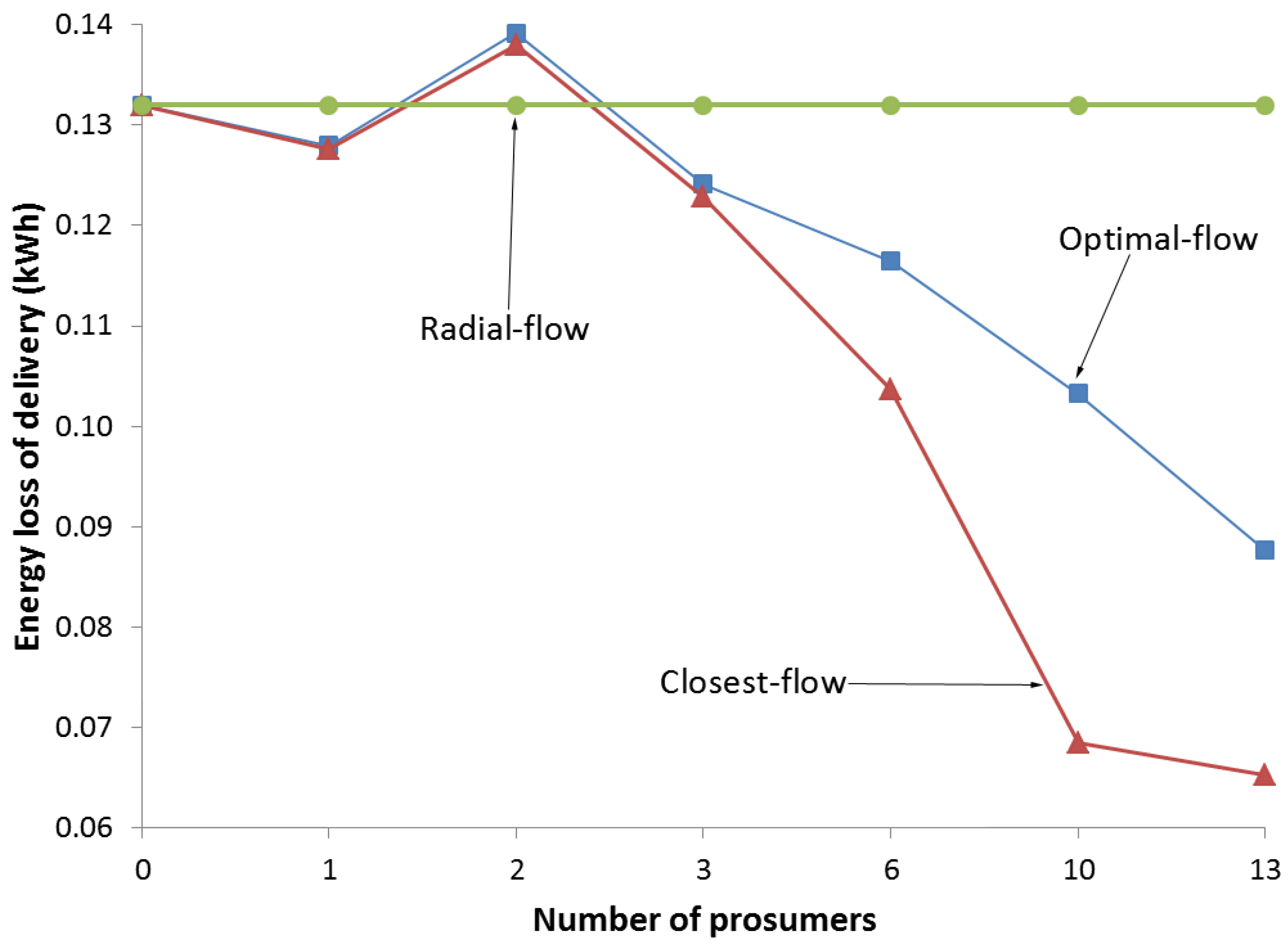
One aim of our study is to decrease energy loss of delivery in the test feeder. The performance of energy loss reduction is shown in Figure 3. For the Optimal-flow Case and the Closest-flow Case, the overall trend of energy loss is decreasing with the increase of the number of prosumers. Energy loss in this figure is based on transmitting the same amount of energy in the three evaluation cases. For the Optimal-flow Case and the Closest-flow Case, the loss of buying energy from prosumers and the loss of buying energy from the electric utility are both counted. With the rising number of prosumers, the amount of energy transmitted from the electric utility decreases (shown in Figure 4 and Figure 5) and the amount of energy flowing as the proposed solution increases. Then, the efficiency of energy loss reduction in the test feeder is improved. This finding means that the solution proposed in this study outperform the baseline (traditional power system) in reducing energy loss of delivery.
In Figure 3, there are peaks of energy loss for both the Optimal-flow Case and the Closest-flow Case and the peaks are beyond the baseline. This happens when the number of prosumers, denoted by M, is 2. This can be explained with the consumers’ preference to buy energy from prosumers in our simulation. Consumers still would buy energy from prosumers when the energy loss of buying energy from prosumers is greater than the cost of buying energy from the electric utility. When , the influence of the case mentioned above is significant. This can cause the increase of energy loss. For example, if we assume that the prosumers are Node 634 and Node 646, and one of consumers is Node 611; that energy from the electric utility is injected via Node 650, then for Node 611, buying energy from Node 634 or Node 646 obviously has more energy losses than from the electric utility. When , there is only about of energy in the test feeder provided by the prosumer (shown in Figure 4). Compared to of energy provided by the prosumers when , the influence of the case mentioned above is limited. When , there are more choices for consumers to select prosumers. Therefore, the consumers are able to buy energy from the prosumers with lower energy loss than the situation of .
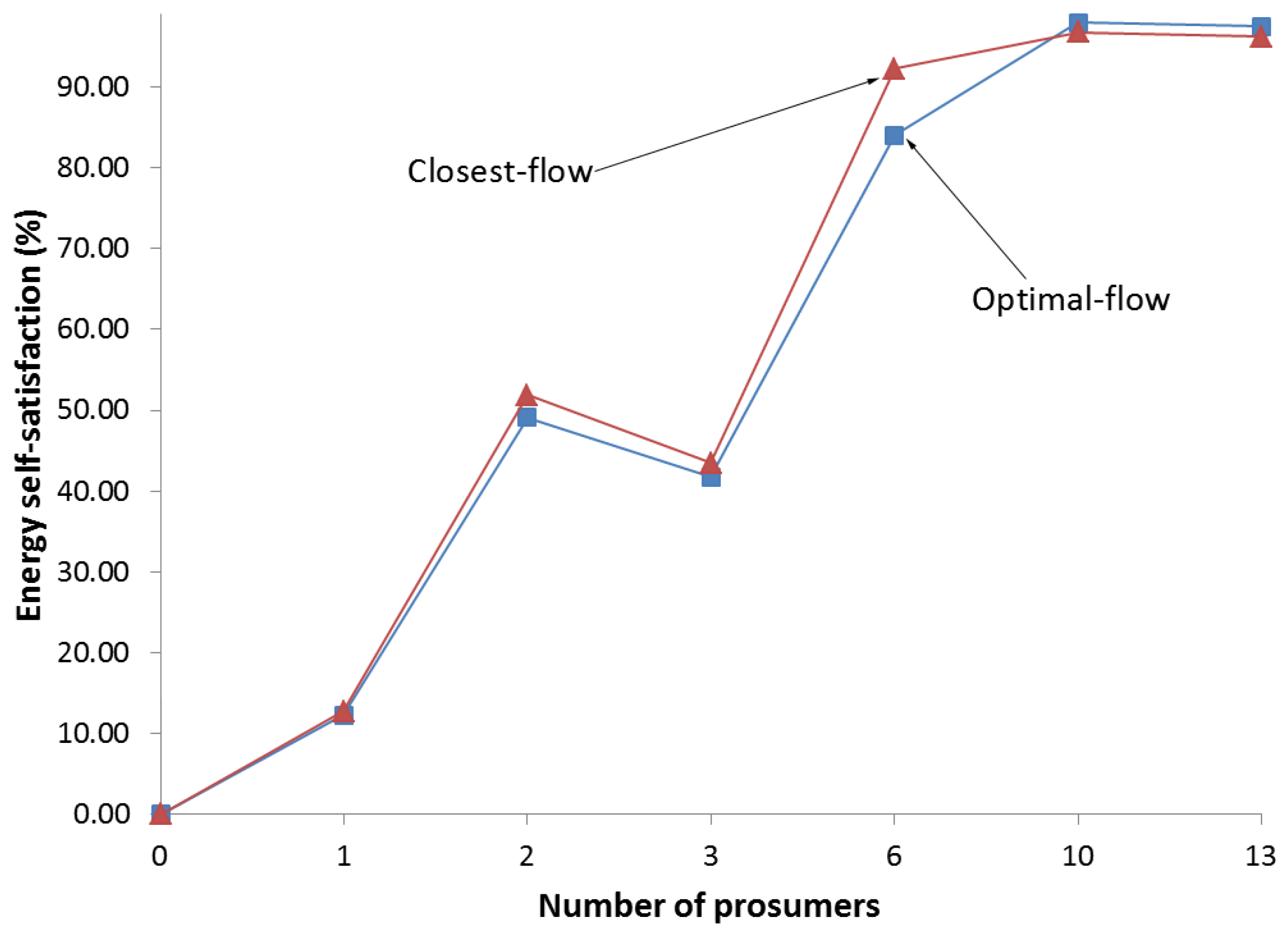
Comparing to the traditional power system, the Prosumer-involved Smart Grid has a considerable advantage in terms of improving independence from centralised energy generation and central energy providers, Figure 4. The upward trend in proportion of energy self-satisfaction is shown in Figure 4. In this figure, the proportion of energy that provided by prosumers to the total energy consumption increases with the rising number of prosumers in both cases of the Optimal-flow and the Closest-flow. Because the increasing number of prosumers causes the increase of distributed energy generation and decentralised energy exchange among end-users. For the Radial-flow Case (i.e., baseline), the energy self-satisfaction is always 0, overlapping with the X axis. On the contrary, energy provided by the electric utility decreases when we add prosumers. This can be observed in Figure 5. The reason of this descending trend is the same as the reason of the ascending trend of energy self-satisfaction. Moreover, the results of the Optimal-flow Case and the Closest-flow Case are lower than the baseline. This finding supports that the solution improves independence from centralised energy generation and central energy providers.
We also measured the excess energy that is sent to the electric utility. The excess energy shown in Figure 6 is prosumers’ energy that is not sold or transmitted to other end-users. For the Radial-flow Case (i.e., baseline), the excess energy is always 0, overlapping with the X axis. For other two cases, it significantly increases with the number of prosumers. The reason of this ascending trend is similar to the one of energy self-satisfaction. Besides, most parts of the two curves in Figure 6 overlap. It means that different patterns of energy flows have no influence on this metric.
Another aim of our study is to save energy costs for end-users. The energy cost is the total amount of money paid by the end-user for buying energy over a day. The results in Figure 7 show a dropping trend of average energy costs per end-user with the rising number of prosumers. The results of the Optimal-flow Case and the Closest-flow Case are both lower than the baseline. Since the price formation is beyond the scope of this paper, we simply consider that the renewable energy produced by prosumers has different prices from the energy provided by the electric utility; grid fees, accounting risks, structuring of profiles and taxes are considered to be fixed. Thus, renewable energy produced by prosumers is sold with lower price than energy provided by the electric utility in the Prosumer-involved Smart Grid. Therefore, energy costs of end-users are reduced when more prosumers are involved in the test feeder and more renewable energy is exchanged among end-users.
The figures give an indication of the overall performance of the Optimal-flow Case and the Closest-flow Case and how these significantly improve on the current baseline (i.e., the Radial-flow Case). To clearly indicate the improvement, numerical data of the evaluation based on four metrics are shown in Table 2. We calculate the percentage of the maximum reduction based on the baseline for three metrics, including energy loss of delivery, average energy costs and energy provided by the electric utility. The maximum values of energy self-satisfaction proportion are also shown in this table. Compared to the baseline, the maximum reduction of energy loss is achieved by the Closest-flow Case. The Optimal-flow Case maximumly reduces energy provided by the electric utility by . It also obtains the maximum proportion of energy self-satisfaction that is . The maximum reduction of average energy costs per end-user is achieved in both cases.
To compare the Optimal-flow Case with the Closest-flow Case, based to the data in Table 2, we design Figure 8. The figure highlights how these two evaluation cases have the same performance in the maximum reduction of average energy costs per end-user. They also have very close performance in the maximum reduction of energy provided by the electric utility and the maximum proportion of energy self-satisfaction. However, the Optimal-flow Case slightly exceeds the Closest-flow Case in these two metrics. On the other hand, the Closest-flow Case significantly outperforms the Optimal-flow Case in energy loss of delivery.
For energy loss of delivery, the Closest-flow Case obviously outperforms the Optimal-flow Case in Figure 3 and Figure 8. The reason of this outcome is linked to the use of a radial test feeder to test the solution. As described in Section 6.1, the energy flow pattern of the Closest-flow Case approximates to the realistic situation when delivering energy in the test feeder. In the realistic situation, the test feeder has the radial topology. Thus, the Closest-flow Case is designed for the radial test feeder. It may therefore have better performance than the Optimal-flow Case in this test feeder. However, the ideal test platform for the Optimal-flow Case is a test feeder with a more meshed topology. In the radial network, there is only one path between each pair of nodes. This negatively influences the optimisation of delivery paths proposed in Section 4.3. For example, if in Figure 2 Node 634 transmits energy to Node 611, the energy flow travels on the longest path in the test feeder and blocks energy transit between other nodes. The blocked consumers have to buy energy from the electric utility. This may increase energy loss of delivery. When the number of prosumers rises, the number of nodes involved in decentralised energy exchange increases. Then, the negative influence of the radial topology may therefore become apparent.
7. Conclusions
We proposed a novel strategy for optimising decentralised energy exchange based on the Prosumer-involved Smart Grid. The optimisation strategy considers renewable energy production of prosumers, energy loss of delivery, topology of the distribution network, and physical constraints including ampacity of electric lines and directions of energy flows. A mathematical model of the optimisation problem and a P2P model of the Prosumer-involved Smart Grid are central to the present study. We designed algorithms and evaluated them by building a simulation programme and running it on three representative cases. The simulation results prove the effectiveness of our solution. Compared with the traditional power system, the maximum reduction of energy loss, energy costs, and energy provided by the electric utility based on the proposed solution can achieve , , and , in each case. Besides, the maximum proportion of energy self-satisfaction in the test feeder approaches and there is large amount of excess energy sent to the electric utility. The study does provide further evidence to the potential of having an open energy market for prosumers, as this is more efficient and it makes become a prosumer economically more attractive than the current model where the utilities buy back the produced energy.
The proposed algorithms are based on heuristic methods. The final results provided by our solution are near-optimal. However, the focus of this paper is not on the optimality of energy flows, but on the comparison of distribution solutions. In the future work, it is our intention to analyse the optimality of the solution and the influence of the topology with respect to the proposed model.
In the open energy market mentioned above, transaction costs for buying and selling energy should be considered. The transaction costs could be significantly reduced if the number of transactions is very high and thus result in micropayment per transaction. This is for instance the case in the domain of Cloud Computing and Service-Oriented Architectures [38,39]. Our current study focuses on the distribution costs which are additive to the transaction costs. A further study of the transaction costs is left for future work.
To gain further insights in attractive future Smart Grid models, we will consider introducing distributed energy storage systems (DESS, such as home batteries and electric vehicles) and adding the optimisation of the charge/discharge cycle to the model. Because there is large amount of excess energy sent to the electric utility (Figure 6). With DESS, prosumers are enabled to decide whether the excess energy should be sold for an immediate profit or stored for later use.
Acknowledgments
The authors are grateful to Giuliano Andrea Pagani for the fruitful discussions and suggestions of the assessment metrics. The authors are grateful to Laura Fiorini for the fruitful discussions about Power Systems Engineering. Ang Sha is supported by the China Scholarship Council (CSC) with grant number 201409110097.
Author Contributions
Ang Sha performed the problem modelling, algorithm design, simulation implementation, evaluation, result analysis, and constructed the manuscript. Marco Aiello supervised the research, provided key suggestions on the problem modelling, simulation and evaluation, and revised the manuscript.
Conflicts of Interest
The authors declare no conflict of interest. The founding sponsors had no role in the design of the study; in the collection, analyses, or interpretation of data; in the writing of the manuscript, and in the decision to publish the results.
References
- The Smart Grid: An Introduction. Available online: http://energy.gov/oe/downloads/smart-grid- introduction-0 (accessed on 30 April 2016).
- Yu, X.; Cecati, C.; Dillon, T.; Simões, M. The New Frontier of Smart Grids. IEEE Ind. Electron. Mag. 2011, 5, 49–63. [Google Scholar] [CrossRef]
- Cecati, C.; Citro, C.; Siano, P. Combined Operations of Renewable Energy Systems and Responsive Demand in a Smart Grid. IEEE Trans. Sustain. Energy 2011, 2, 468–476. [Google Scholar] [CrossRef]
- Wu, Y.; Lau, V.; Tsang, D.; Qian, L.; Meng, L. Optimal Exploitation of Renewable Energy for Residential Smart Grid with Supply-demand Model. In Proceedings of the 7th International ICST Conference on Communications and Networking in China (CHINACOM), Kunming, China, 8–10 August 2012; pp. 87–92.
- Guo, Y.; Pan, M.; Fang, Y. Optimal Power Management of Residential Customers in the Smart Grid. IEEE Trans. Parallel Distr. Syst. 2012, 23, 1593–1606. [Google Scholar] [CrossRef]
- Li, Y.; Wang, Y.; Nazarian, S.; Pedram, M. A Nested Game-based Optimization Framework for Electricity Retailers in the Smart Grid with Residential Users and PEVs. In Proceedings of the 2013 IEEE Online Conference on Green Communications (GreenCom), Piscataway, NJ, USA, 29–31 October 2013; pp. 157–162.
- Aghaei, J.; Alizadeh, M.I. Demand Response in Smart Electricity Grids Equipped with Renewable Energy Sources: A Review. Renew. Sustain. Energy Rev. 2013, 18, 64–72. [Google Scholar] [CrossRef]
- Wang, Y.; Lin, X.; Pedram, M. A Stackelberg Game-Based Optimization Framework of the Smart Grid With Distributed PV Power Generations and Data Centers. IEEE Trans. Energy Convers. 2014, 29, 978–987. [Google Scholar] [CrossRef]
- Broeer, T.; Fuller, J.; Tuffner, F.; Chassin, D.; Djilali, N. Modeling Framework and Validation of a Smart Grid and Demand Response System for Wind Power Integration. Appl. Energy 2014, 113, 199–207. [Google Scholar] [CrossRef]
- Taniguchi, T.; Takata, T.; Fukui, Y.; Kawasaki, K. Convergent Double Auction Mechanism for a Prosumers’ Decentralized Smart Grid. Energies 2015, 8, 12342–12361. [Google Scholar] [CrossRef]
- Kim, S.W.; Kim, J.; Jin, Y.G.; Yoon, Y.T. Optimal Bidding Strategy for Renewable Microgrid with Active Network Management. Energies 2016, 9, 48. [Google Scholar] [CrossRef]
- Capodieci, N.; Pagani, G.A.; Cabri, G.; Aiello, M. Smart Meter Aware Domestic Energy Trading Agents. In Proceedings of the 2011 IEEMC 11 Workshop on E-energy Market Challenge, Karlsruhe, Germany, 14–18 June 2011; pp. 1–10.
- Capodieci, N.; Pagani, G.A.; Cabri, G.; Aiello, M. An Adaptive Agent-based System for Deregulated Smart Grids. In Service Oriented Computing and Applications; Springer: London, UK, 2015; pp. 1–21. [Google Scholar]
- Kok, K. Multi-agent Coordination in the Electricity Grid, from Concept Towards Market Introduction. In Proceedings of the 9th International Conference on Autonomous Agents and Multiagent Systems: Industry Track, Toronto, ON, Canada, 9–14 May 2010; International Foundation for Autonomous Agents and Multiagent Systems: Richland, SC, USA, 10 May 2010; pp. 1681–1688. [Google Scholar]
- Bliek, F.; van den Noort, A.; Roossien, B.; Kamphuis, R.; de Wit, J.; van der Velde, J.; Eijgelaar, M. PowerMatching City, A Living Lab Smart Grid Demonstration. In Proceedings of the IEEE PES Innovative Smart Grid Technologies Conference Europe (ISGT Europe), Gothenburg, Sweden, 11–13 October 2010; pp. 1–8.
- Kok, J.K.; Scheepers, M.J.J.; Kamphuis, I.G. Intelligence in Electricity Networks for Embedding Renewables and Distributed Generation. In Intelligent Infrastructures; Negenborn, R.R., Lukszo, Z., Hellendoorn, H., Eds.; Springer Netherlands: Dordrecht, The Netherlands, 2010; pp. 179–209. [Google Scholar]
- Kok, K. The PowerMatcher: Smart Coordination for the Smart Electricity Grid; TNO: The Hague, The Netherlands, 2013; pp. 241–250. [Google Scholar]
- Mocanu, E.; Aduda, K.; Nguyen, P.; Boxem, G.; Zeiler, W.; Gibescu, M.; Kling, W. Optimizing the Energy Exchange between the Smart Grid and Building Systems. In Proceedings of the 2014 49th International Universities Power Engineering Conference (UPEC), Cluj-Napoca, Romania, 2–5 September 2014; pp. 1–6.
- Han, T.; Ansari, N. Smart Grid Enabled Mobile Networks: Jointly Optimizing BS Operation and Power Distribution. In Proceedings of the 2014 IEEE International Conference on Communications (ICC), Sydney, Australia, 10–14 June 2014; pp. 2624–2629.
- Kim, B.; Lavrova, O. Optimal Power Flow and Energy-sharing among Multi-agent Smart Buildings in the Smart Grid. In Proceedings of the 2013 IEEE Energytech, Cleveland, OH, USA, 21–23 May 2013; pp. 1–5.
- HomChaudhuri, B.; Kumar, M.; Devabhaktuni, V. Market Based Approach for Solving Optimal Power Flow Problem in Smart Grid. In Proceedings of the American Control Conference (ACC), Montreal, QC, Canada, 27–29 June 2012; pp. 3095–3100.
- Gemine, Q.; Ernst, D.; Louveaux, Q.; Cornélusse, B. Relaxations for Multi-period Optimal Power Flow Problems with Discrete Decision Variables. In Proceedings of the Power Systems Computation Conference (PSCC), Wroclaw, Poland, 18–22 August 2014; pp. 1–7.
- Hauswirth, A.; Summers, T.; Warrington, J.; Lygeros, J.; Kettner, A.; Brenzikofer, A. A Modular AC Optimal Power Flow Implementation for Distribution Grid Planning. In Proceedings of the 2015 IEEE Eindhoven PowerTech, Eindhoven, The Netherlands, 29 June–2 July 2015; pp. 1–6.
- Pagani, G.A.; Aiello, M. From the Grid to the Smart Grid, Topologically. Phys. A Stat. Mech. Appl. 2016, 449, 160–175. [Google Scholar] [CrossRef]
- Brown, R. Impact of Smart Grid on Distribution System Design. In Proceedings of the 2008 IEEE Power and Energy Society General Meeting—Conversion and Delivery of Electrical Energy in the 21st Century, Pittsburgh, PA, USA, 20–24 July 2008; pp. 1–4.
- Dugan, R.; Arritt, R.; McDermott, T.; Brahma, S.; Schneider, K. Distribution System Analysis to Support the Smart Grid. In Proceedings of the 2010 IEEE Power and Energy Society General Meeting, Minneapolis, MN, USA, 25–29 July 2010; pp. 1–8.
- Pagani, G.A.; Aiello, M. Power Grid Complex Network Evolutions for the Smart Grid. Phys. A Stat. Mech. Appl. 2014, 396, 248–266. [Google Scholar] [CrossRef]
- Grigsby, L.L. Electric Power Generation, Transmission, and Distribution, 2nd ed.; CRC Press: Boca Raton, FL, USA, 2007. [Google Scholar]
- Daintith, J. A Dictionary of Physics, 6th ed.; Oxford University Press: Oxford, UK, 2009. [Google Scholar]
- Cormen, T.; Leiserson, C.; Rivest, R.; Stein, C. Introduction to Algorithms, 3rd ed.; MIT Press: Cambridge, MA, USA, 2009; p. 658. [Google Scholar]
- Daily Data from the Weather in the Netherlands. Available online: http://www.knmi.nl/nederland-nu/ klimatologie/daggegevens (accessed on 7 January 2016).
- Groningen, Netherlands—Sunrise, Sunset, and Daylength. 2015. Available online: http://www. timeanddate.com/sun/netherlands/groningen?month=1&year=2015 (accessed on 7 January 2016).
- Energy Consumption of Small Customers in the Netherlands. Available online: http://www.liander.nl/ over-liander/innovatie/open-data/data (accessed on 7 January 2016).
- Back Delivery Fees in the Netherlands. Available online: http://www.energieleveranciers.nl/zonnepanelen/ terugleververgoeding-zonnepanelen (accessed on 8 April 2016).
- Kersting, W.H. Radial Distribution Test Feeders. In Proceedings of the 2001 IEEE Power Engineering Society Winter Meeting, Columbus, OH, USA, 28 January–1 February, 2001; Volume 2, pp. 908–912.
- Grogg, K. Harvesting the Wind: The Physics of Wind Turbines. In Physics and Astronomy Comps Papers; Carleton College: Northfield, MN, USA, 2005; p. 7. [Google Scholar]
- Law, A. Simulation Modeling and Analysis, 4th ed.; McGraw-Hill: New York, NY, USA, 2007. [Google Scholar]
- Kossmann, D.; Kraska, T.; Loesing, S. An Evaluation of Alternative Architectures for Transaction Processing in the Cloud. In Proceedings of the 2010 ACM SIGMOD International Conference on Management of Data, Indianapolis, IN, USA, 6–11 June 2010; ACM: New York, NY, USA, 2010; pp. 579–590. [Google Scholar]
- Roberson, J.; Greene, W. System and Method for Implementing Frictionless Micropayments for Consumable Services. U.S. Patent US20030126079 A1, 3 July 2003. [Google Scholar]
Figure 1.
A simple example to describe the procedure of the algorithms proposed in this section.
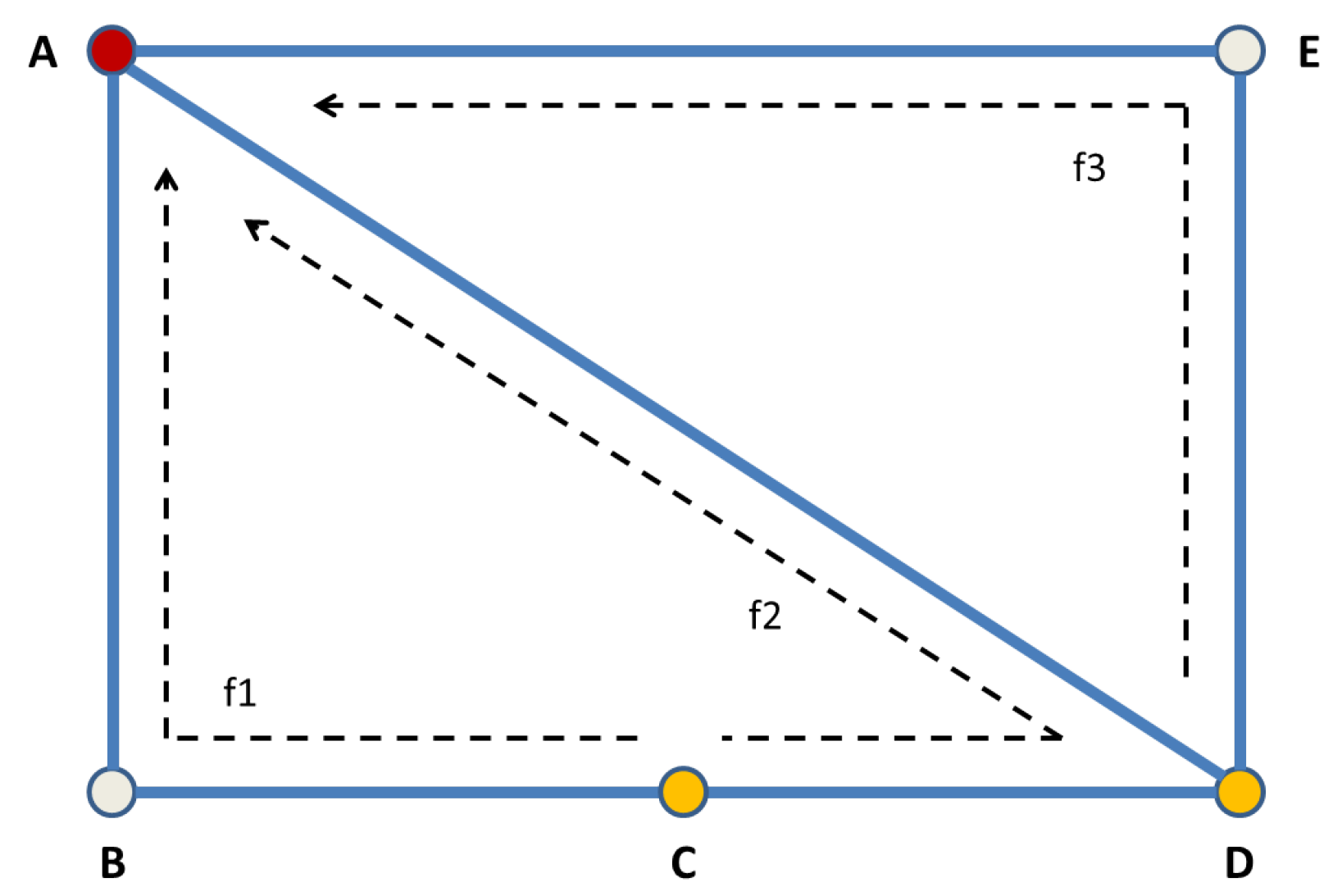
Figure 2.
The modified IEEE 13-bus test feeder.

Figure 3.
Energy loss of delivery in the test feeder.

Figure 4.
Proportion of energy self-satisfaction.

Figure 5.
Energy provided by the electric utility.
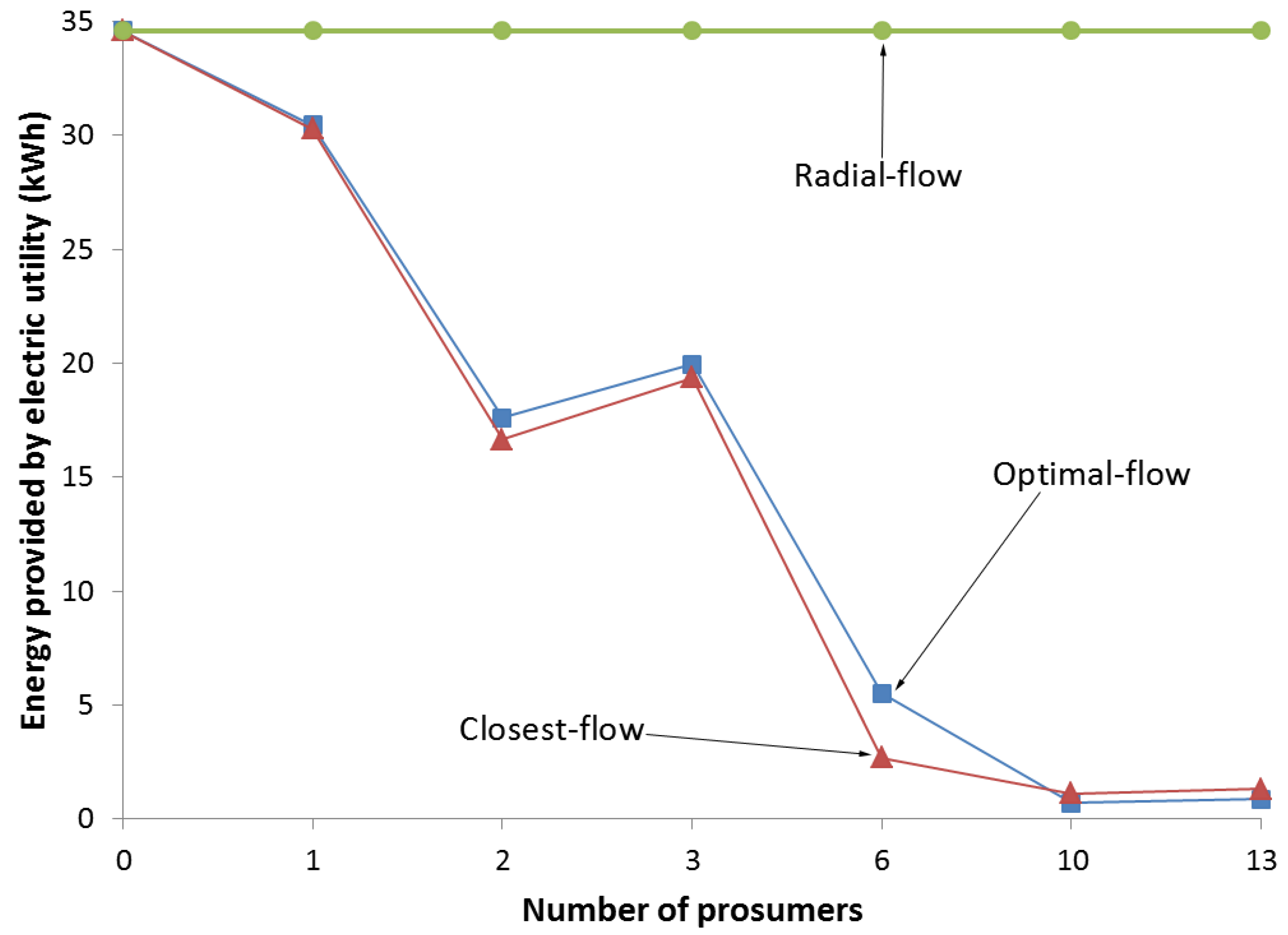
Figure 6.
Excess energy sent to the electric utility.
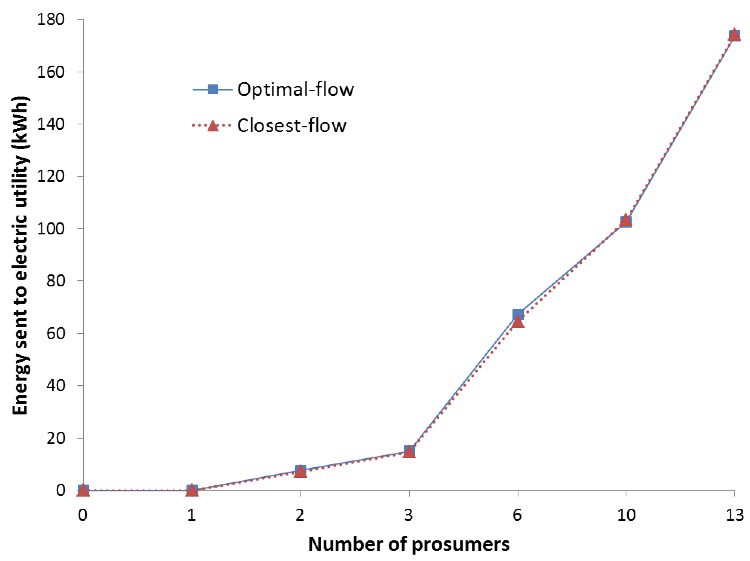
Figure 7.
Average energy costs per end-user per day.
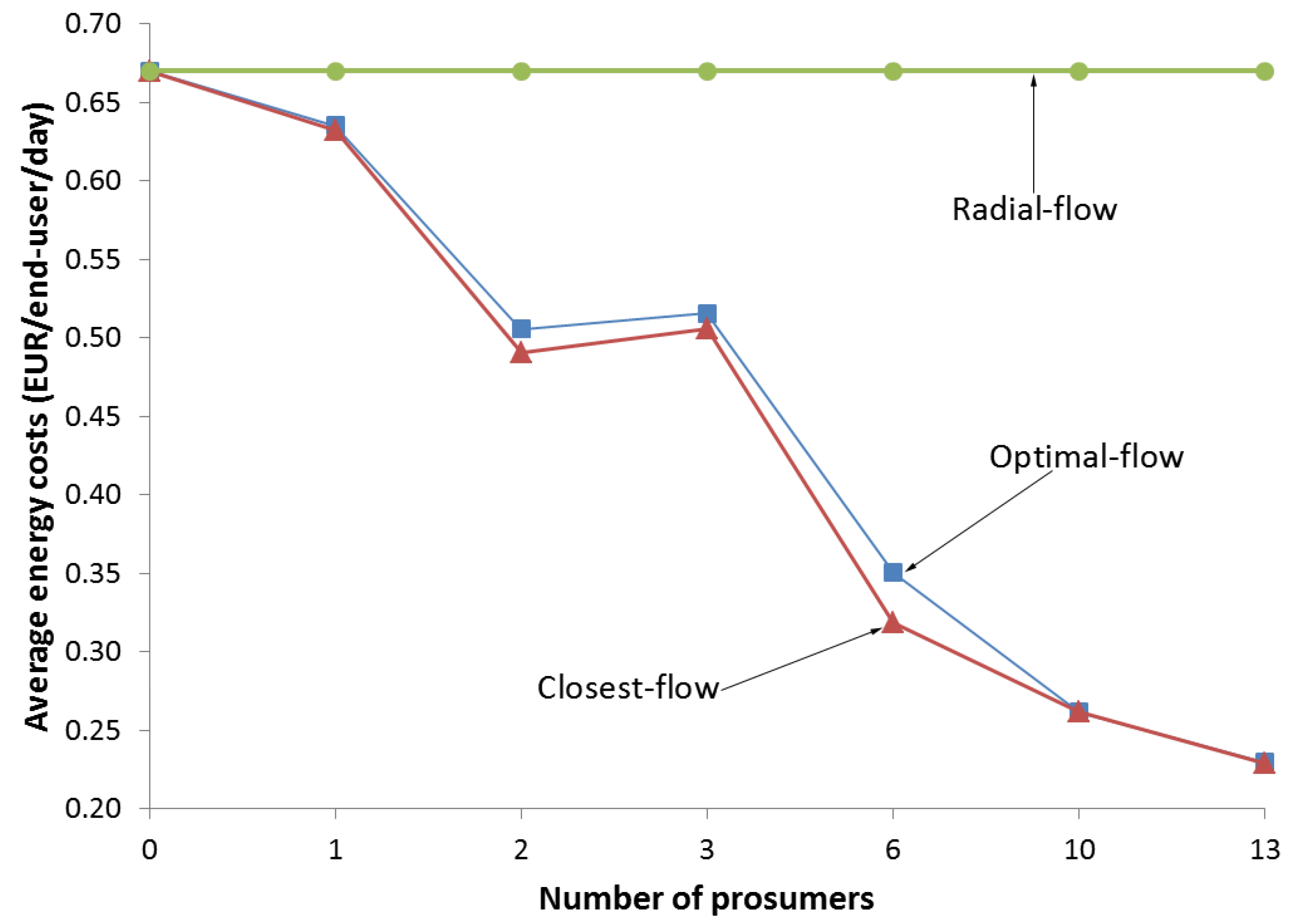
Figure 8.
Comparison with assessment metrics of Optimal-flow Case and Closest-flow Case.


| Symbol | Stand for | Unit |
|---|---|---|
| P | electric power | kW (kilo watt) |
| E | electrical energy | kWh (kilo watt hour) |
| I | electric current | A (ampere) |
| V | voltage | kV (kilo volt) |
| time slot | hour | |
| R | electrical resistance | ohm |
| L | energy loss | Wh (watt hour) |
| Assessment Metrics | Radial-Flow | Optimal-Flow | Closest-Flow |
|---|---|---|---|
| Baseline | Maximum reduced | Maximum reduced | |
| Energy loss of delivery | 0.13 kWh | 33% | 51% |
| Average energy costs | 0.67 EUR | 66% | 66% |
| Energy from electric utility | 34.6 kWh | 97.5% | 96% |
| Baseline | Maximum proportion | Maximum proportion | |
| Energy self-satisfaction | 0 | 98% | 96.8% |
© 2016 by the authors; licensee MDPI, Basel, Switzerland. This article is an open access article distributed under the terms and conditions of the Creative Commons Attribution (CC-BY) license (http://creativecommons.org/licenses/by/4.0/).
Share and Cite
MDPI and ACS Style
Sha, A.; Aiello, M. A Novel Strategy for Optimising Decentralised Energy Exchange for Prosumers. Energies 2016, 9, 554. https://doi.org/10.3390/en9070554
AMA Style
Sha A, Aiello M. A Novel Strategy for Optimising Decentralised Energy Exchange for Prosumers. Energies. 2016; 9(7):554. https://doi.org/10.3390/en9070554
Chicago/Turabian StyleSha, Ang, and Marco Aiello. 2016. "A Novel Strategy for Optimising Decentralised Energy Exchange for Prosumers" Energies 9, no. 7: 554. https://doi.org/10.3390/en9070554
Note that from the first issue of 2016, this journal uses article numbers instead of page numbers. See further details here.