Reliability Analysis of Distribution Systems with Photovoltaic Generation Using a Power Flow Simulator and a Parallel Monte Carlo Approach

Abstract

This paper presents a Monte Carlo approach for reliability assessment of distribution systems with distributed generation using parallel computing. The calculations are carried out with a royalty-free power flow simulator, OpenDSS (Open Distribution System Simulator). The procedure has been implemented in an environment in which OpenDSS is driven from MATLAB. The test system is an overhead distribution system represented by means of a three-phase model that includes protective devices. The paper details the implemented procedure, which can be applied to systems with or without distributed generation, includes an illustrative case study and summarizes the results derived from the analysis of the test system during one year. The goal is to evaluate the test system performance considering different scenarios with different level of system automation and reconfiguration, and assess the impact that distributed photovoltaic generation can have on that performance. Several reliability indices, including those related to the impact of distributed generation, are obtained for every scenario.

1. Introduction

It is widely accepted that distributed generation (DG) can have a positive impact on the distribution system since it can support voltage, reduce losses, provide backup power, provide ancillary services, or defer distribution system upgrade [1,2]. However, the connection of generation to the distribution system can cause miscoordination of protection devices and, if not properly handled, reduce reliability and power quality. Although distributed generation is often presented as a solution for reliability improvement, the fact is that such assumption is not always accepted or supported, see for instance [3].

Two main modes of DG connection can be distinguished: (1) DG operates as a backup source within a microgrid; (2) DG operates in parallel with the distribution system. In the first case, the generation units are locally operated and can be allowed to inject power to the system; if they are correctly controlled, they can have a positive impact on distribution system reliability [4]. A generation unit operating in parallel to the system can be forced to be disconnected in case of system fault, so the benefit to the system reliability can be negative [3,4].

This paper presents an expanded version of a procedure for reliability of distribution systems developed by the authors and presented in [5]. The new procedure aims at evaluating the reliability of distribution systems with distributed generation using a Monte Carlo approach, assuming the DG units are operating in parallel to the distribution system, and takes advantage of the computing capabilities of a multicore environment.

The software application used for this purpose is OpenDSS [6], a freely available tool that allows users to represent the distribution system with a great accuracy and carry out the calculations over an arbitrary time period using a variable time step size. OpenDSS can be used as either a stand-alone executable program or as a COM-DLL (Component Object Model-Dynamic Linked Library) that can be driven from some software platforms; e.g., MATLAB [6,7].

The reliability of distribution systems with distributed generation has already been analyzed in a significant number of works; see, for instance [8,9,10,11,12,13,14,15,16,17,18,19,20]. A summary of the methods proposed until 2009 was presented in [21]. The approach detailed in this work uses a power flow simulator whose model includes the protection system, see [5]. The system model assumes that there are no microgrids in the distribution network, only photovoltaic (PV) generation is connected and an anti-islanding protection is installed at the interconnection of all PV generators.

The application of a power flow simulator as OpenDSS in reliability studies has some advantages since it can be used to illustrate how the presence of distributed generation can favorably impact the performance of a distribution network after a fault.

Section 2 summarizes the main aspects of the Monte Carlo procedure and its implementation in MATLAB/OpenDSS. The test system used in this paper is presented in Section 3. The modeling guidelines and parameters required for reliability studies are discussed and provided in Section 4. Section 5 details a case study whose main goal is to illustrate the way in which the approach proposed in this paper is used to assess the reliability of the distribution system. The main results derived from the reliability analysis of the test system are summarized in Section 6; that section also proposes reliability indices to assess the impact of photovoltaic generation and discusses the circumstances under which the connection of generation units to the distribution system can have a positive impact in its reliability. The main characteristics of the multicore computing installation used in this work were summarized in [5].

2. Procedure for Distribution Reliability Calculation

2.1. Description of the Procedure

The new procedure may be defined as a parallel Monte Carlo method aimed at estimating reliability indices of distribution systems with DG. Input data include system parameters (i.e., network topology, component parameters, including setting of protection devices) and yearly variation of load and generation. Random variables to be generated during the application of the Monte Carlo method implemented for this work are those related to failures rates, fault characterization (location, time of occurrence, duration, type), and reconfiguration times. The main steps of the procedure may be summarized as follows (see also [5]):

• Run the test system during one year using time-based power flow simulation and a constant time step (e.g., 1 h). This run, known in this work as base case, provides basic information (e.g., energy values) that will be used for later calculations. Depending on the system under study, the simulation can be carried out with or without distributed generation.
• Estimate in advance all the random values related to the faults/failures to be simulated (location/component, time of occurrence, duration, type) for one year.
• Run the test system again but considering now the possibility of fault and/or equipment failure. Regardless of the location, type and duration of the fault/failure, a protective device will always operate. Reliability indices are updated once this sequence of events is finished.
• Repeat the procedure from Step 2 as many times as required to obtain the information needed for estimating reliability indices.

2.2. Implementation of the Procedure

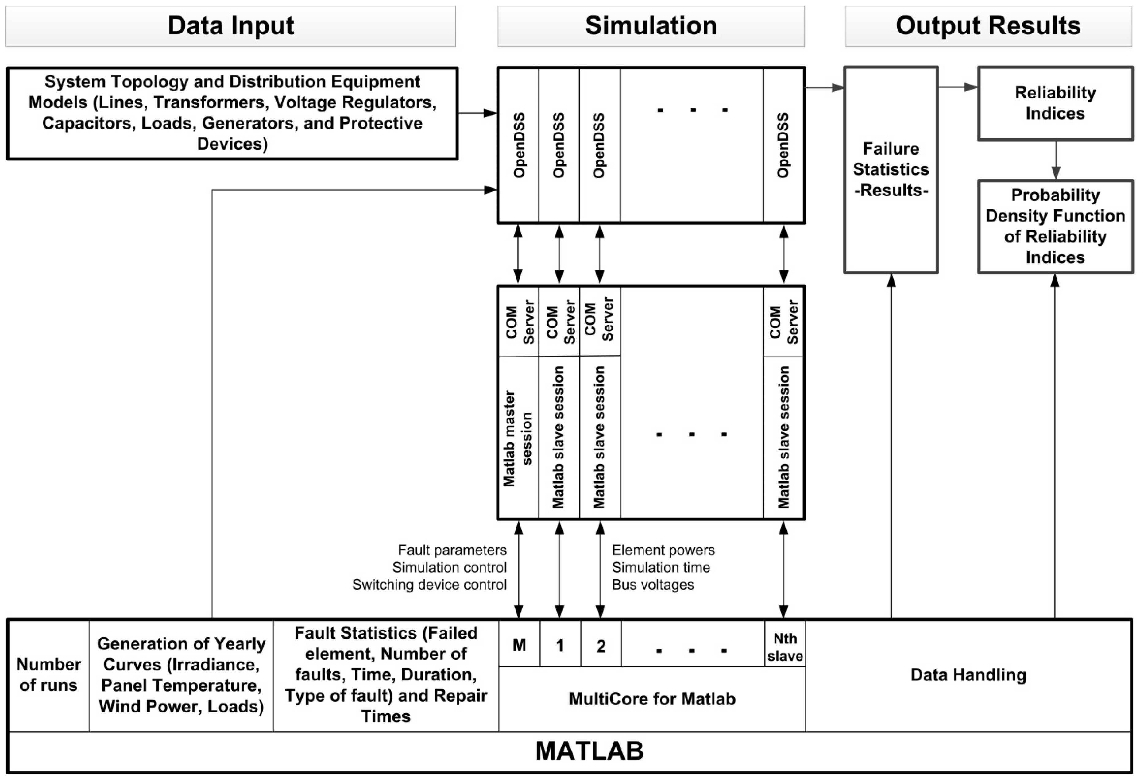
The procedure summarized above has been implemented in MATLAB, which is used to calculate the random variables and control the execution of power flow calculations performed by OpenDSS. Figure 1 shows a diagram with the connections between the different tools used for this work, as well as the information to be inputted to and generated by each tool. Note that all the information required to build and simulate the test system model is generated by means of custom-made applications when OpenDSS capabilities cannot be used. For instance, the algorithms to obtain load and PV generation curves have been implemented in MATLAB, and can be obtained at the time the reliability study is carried out [22,23]. MATLAB also takes care of the simulation results that are needed to calculate reliability indices.

To obtain a probability density function of the reliability indices the procedure is simultaneously run in a multicore computing environment. The procedure schematized in Figure 1 is valid for any number of cores. The system simulated in every core is the same but the number of faults and the characteristics of each fault are different and randomly calculated for each core, see Section 5. MATLAB capabilities can be used to distribute the different runs between cores [24,25]. This work is based on the library developed by Buehren and available at the MathWorks web site [26].

3. Test System

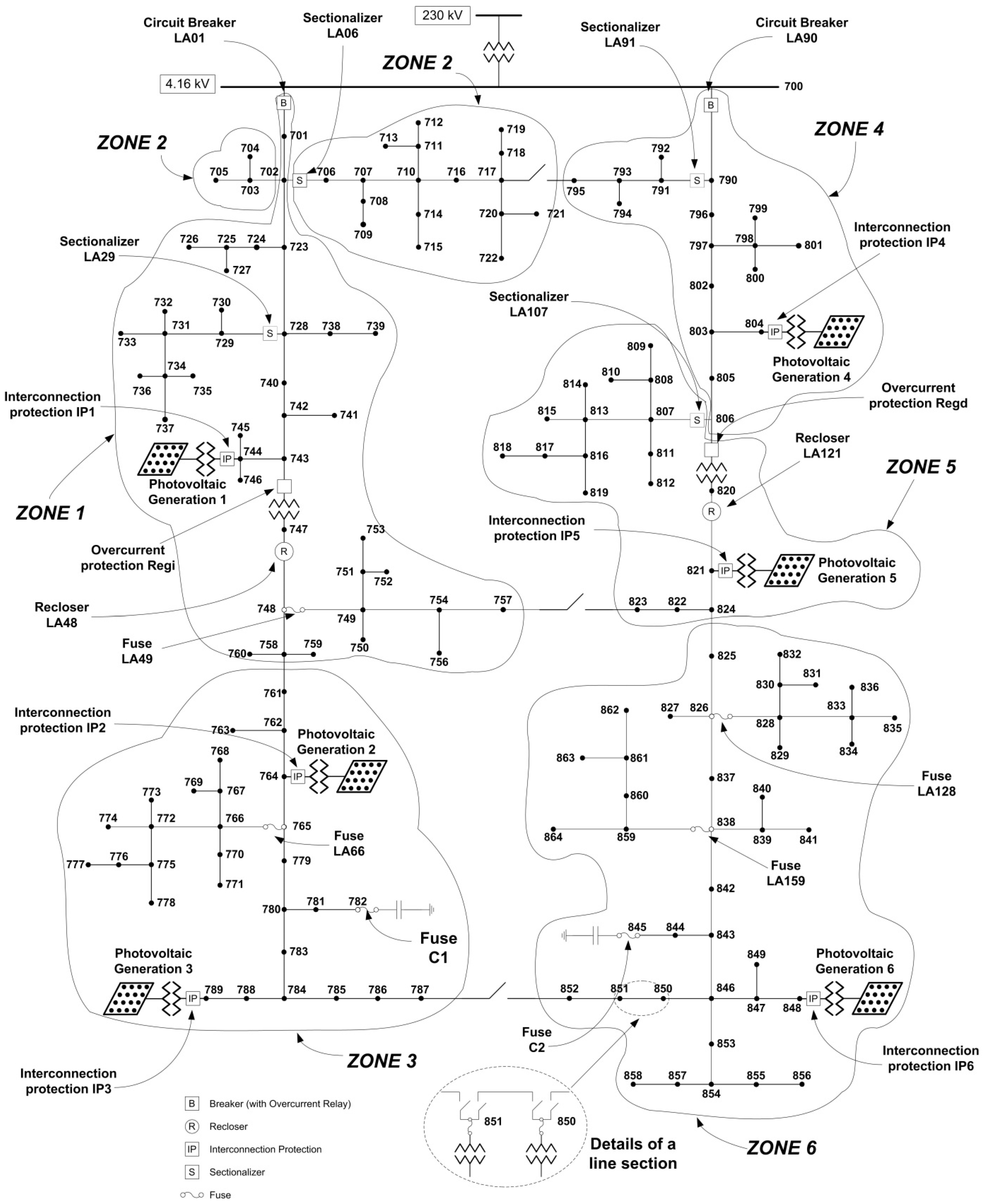
Figure 2 depicts the diagram of the test system. It is a 60-Hz three-phase overhead distribution system based on IEEE test feeders [27]. The figure shows the location of the protective devices and transfer switches that can be used for system reconfiguration and restoration of power. The model includes a simplified representation of the high-voltage system, the substation transformer and all distribution medium voltage (MV)/low voltage (LV) transformers.

All loads are supplied from the LV terminals of distribution transformers. As indicated in the figure, all line sections have switching devices at both terminals. These switches are used to isolate the faulted section and, depending on the automation level in the test system, may be operated either manually or remotely.

The figure shows the zone classification, which is used to obtain fault isolation and repair times, see Section 5. Some important numbers about the test system are given below:

• Rated voltage: 4.16 kV.
• Rated power of substation transformer: 10,000 kVA.
• Rated PV generation power (peak value): 1800 kW.
• Number of load nodes: 107.
• Overall number of customers: 713.
• Average rated power per MV load node: 74.77 kVA.
• Overall line length: 52.1 km.

4. Reliability Model

This section summarizes the guidelines followed to implement the distribution system model and provides the parameters used for the reliability assessment of the test system.

4.1. Modelling Approach

The approach used to represent the system is basically that used in [5] but with distributed generation units and their interconnection protection. In this work the generation is of renewable nature (i.e., photovoltaic) and represented by means of the model available in OpenDSS, with some additional features needed to obtain yearly generation curves. The algorithms implemented to obtain load and generation curves were presented in some previous work by the authors; see [22,23]. By default, it is assumed that PV units only inject active power, and voltage at their terminals is not controlled.

4.2. Parameters for Reliability Assessment

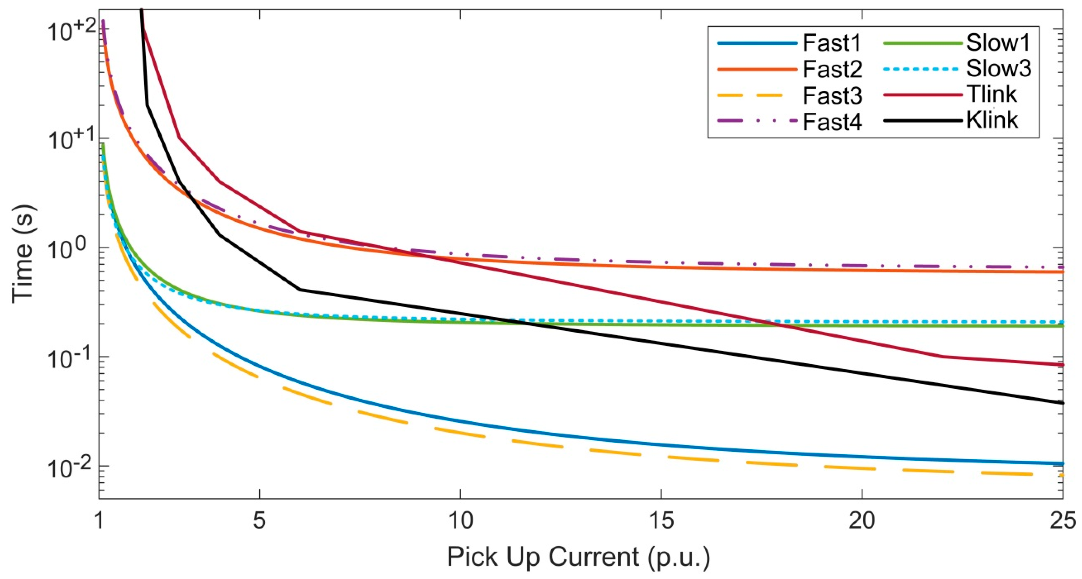
• Protective Devices: Figure 2 shows the type and location of the protective devices installed in the test system. The characteristic time-current curves are similar to those used in [5]; they are shown in Figure 3. The interconnection protection of each generator has over-/undervoltage and overcurrent protection. If a generator is disconnected after a fault, it will be reconnected when normal voltage values at the point of common coupling (PCC) are confirmed (>0.9 pu). On the other hand, it is assumed that PV generators do not suffer any damage during a fault and can be put back in operation as soon as possible.

  Table 1. Main Characteristics of Protective Devices.

  Devices for Feeder Protection
  Protective Device		Current (A)	TC Curve
  			Fast	Slow
  Relay.la01		1000	Fast2	-----
  Relay.la90		640	Fast4	-----
  Recloser.la48		440	Fast1	Slow1
  Recloser.la121		370	Fast3	Slow3
  Overcurrent protection regi		490	Regi	-----
  Overcurrent protection regd		390	Regd	-----
  Fuse.la49		140	Tlink	-----
  Fuse.la66		140	Klink	-----
  Fuse.la128		100	Tlink	-----
  Fuse.la159		140	Klink	-----
  Fuse.c1		30	Klink	-----
  Fuse.c2		50	Klink	-----
  Sectionalizer.la06		115	-----	-----
  Sectionalizer.la29		60	-----	-----
  Sectionalizer.la91		25	-----	-----
  Sectionalizer.la107		80	-----	-----
  Interconnection Protection of PV Plants
  Protected Plant	Over/Undervoltage Protection		Overcurrent Protection
  	Protective Device	Rated Voltage (kV)	Protective Device	Pick-up Current (A)
  Plant1	Relay.LV1	4.16	Relay.PV1	65
  Plant2	Relay.LV2	4.16	Relay.PV2	110
  Plant3	Relay.LV3	4.16	Relay.PV3	130
  Plant4	Relay.LV4	4.16	Relay.PV4	65
  Plant5	Relay.LV5	4.16	Relay.PV5	110
  Plant6	Relay.LV6	4.16	Relay.PV6	130

  provides some information about the devices installed to protect feeders and the interconnection protection of PV plants. Take into account that: (i) reclosers can perform up to three opening operations, two of which use the faster characteristic; (ii) fuses are coordinated using a fuse saving scheme; (iii) sectionalizers count up to two operations before performing an opening action. In all devices with automatic reclosing capabilities, the assumed dead times are 10 and 20 seconds. Except the sectionalizer model, which is a custom-made model, the models used to represent protective devices are those available in OpenDSS.
• Failure Statistics: A fault/failure is fully defined by specifying the faulted component (line, voltage regulator, or capacitor bank), the occurrence time, the duration, and the fault type.

  Table 2. Failure Statistics.

  Time of Occurrence
  Month and Hour			Probability (%)
  Month		January	4
  		February	5
  		March	8
  		April	7
  		May	8
  		June	8
  		July	11
  		August	15
  		September	13
  		October	9
  		November	7
  		December	5
  Hour interval		1–6	30
  		7–12	20
  		13–18	30
  		19–24	20
  Duration
  Type		Probability (%)
  Momentary		75
  Sustained		25
  Type
  Number of phases		Probability (%)
  One-phase—1		70
  Two-Phase—2		25
  Three-Phase—3		5
  Lines
  Zone	Failures
  	Average number (per 100 km)	Standard deviation (per 100 km)	Repair time (hours)
  1	50	12	2
  2	20	7.5	3
  3	30	10	3
  4	45	10	2.5
  5	25	7.5	2.5
  6	20	5	3
  Distribution Transformers
  Failures per year		Repair time (hours)
  0.100		10
  Voltage Regulators
  Failures per year		Repair time (hours)
  0.125		10
  Capacitor Banks
  Failures per year		Repair time (hours)
  0.250		4
  PV Generation Modules
  Module Size (kW)		Failures per year	Repair time (hours)
  100		0.100	10

  shows the statistics assumed for this study. Except for PV generators, the explanations about the way in which this information is applied were given in [5]. The reliability model of a PV plant is rather complex; see, for instance, [4,28,29,30]. Implementing and applying a very detailed model is out of the scope of this study; instead a simplified reliability model is used. All PV generators consist of one or more 100 kW modules, being each module characterized by the same failure rate and repair time. Therefore, the parameters to be defined for reliability assessment of a PV generation unit are the rated power (i.e., the number of 100 kW modules), the failure rate and the mean repair time. A PV plant can totally reduce the power it injects into the system when either the interconnection transformer or all modules fail; the reduction of injected power will be partial when not all PV modules fail. The reliability parameters for the interconnection transformer are those used for any other distribution transformer, while the parameters for characterizing the PV modules are those shown in Table 2. The number of PV module failures in a year will be randomly generated using the failure rate shown in Table 2 and following a Poisson distribution. For every failure the number of failed modules must be determined using also a Poisson distribution. The average repair time is the result of multiplying the number of failed modules by the mean repair time; the actual repair time will be randomly calculated using an exponential distribution.

5. An Illustrative Case Study

5.1. Aim of the Case Study

The occurrence of a system fault or a component failure will cause a sequence of events that may imply protective devices, isolation switches, a system reconfiguration when it is possible and advisable, the repair of the failed component, and the recovery of the original system configuration.

This case study is aimed at illustrating the sequences that can be produced after the occurrence of a fault/failure, the calculations to be made, depending on the system response, as well as the results that can be required for a later estimation of system reliability indices.

5.2. Characteristics of the Case Study

Assume that the characteristics of the case are according to the following information:

• Location: Line section LA93, between load nodes 791 and 793.
• Time of occurrence: 2750 h.
• Type of fault: Phase-to-phase (two-phase fault).
• Faulted phases: A and B.
• Duration: Sustained.
• Scenario: Disconnection and repair of the failed element with load transfer between feeders.

5.3. Sequence of Events

The sequence of events caused by this fault is presented in Figure 4, Figure 5 and Figure 6:

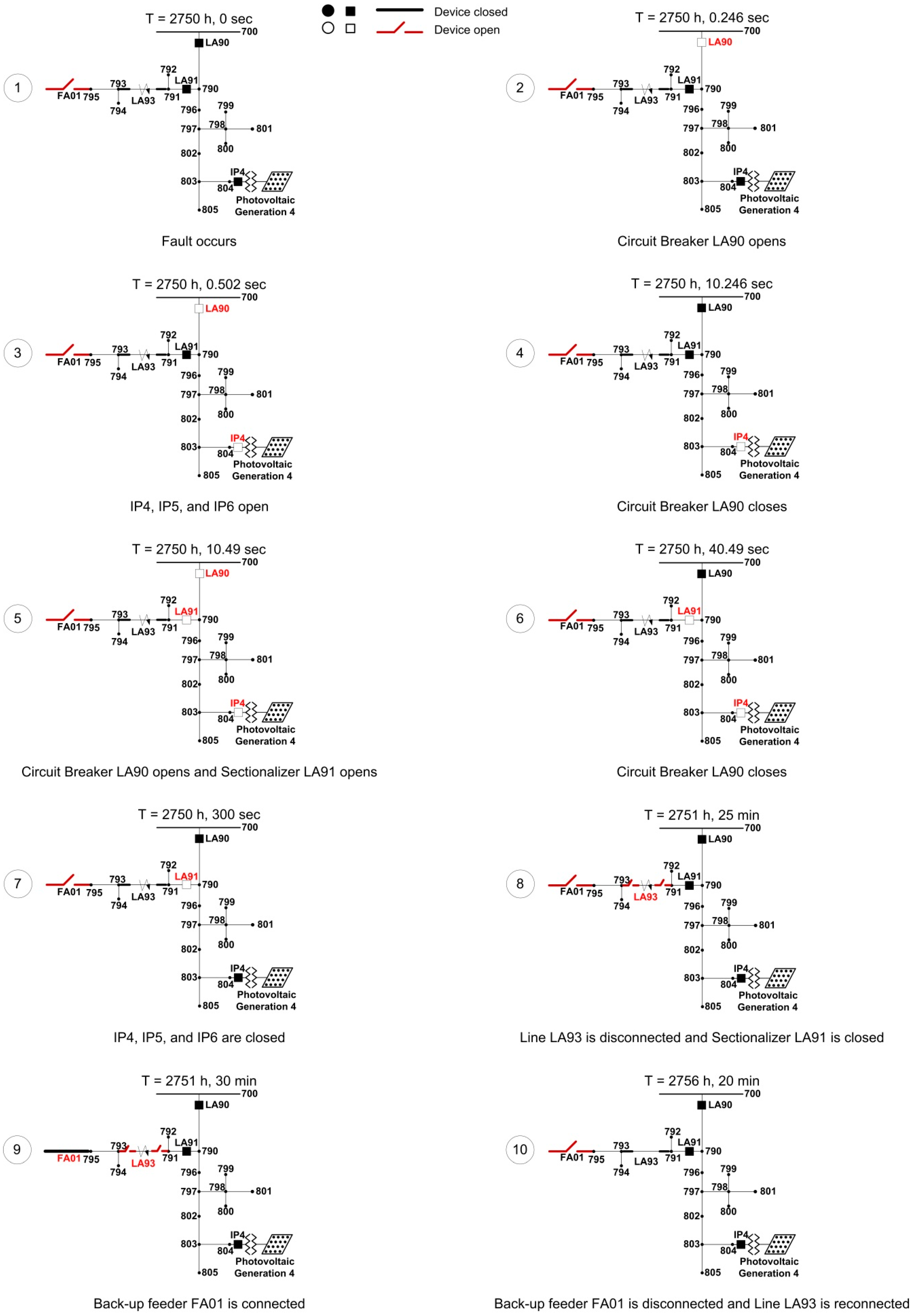
• Figure 4 shows how the configuration of the system changes during the sequence of events caused by the analyzed fault and the status of the various protective devices and switches/disconnectors involved in this case. Remember that, once the fault occurs, the first steps in the sequence of events are caused by the design and settings of the protection system, while the last steps will depend on the performance of the maintenance crew.
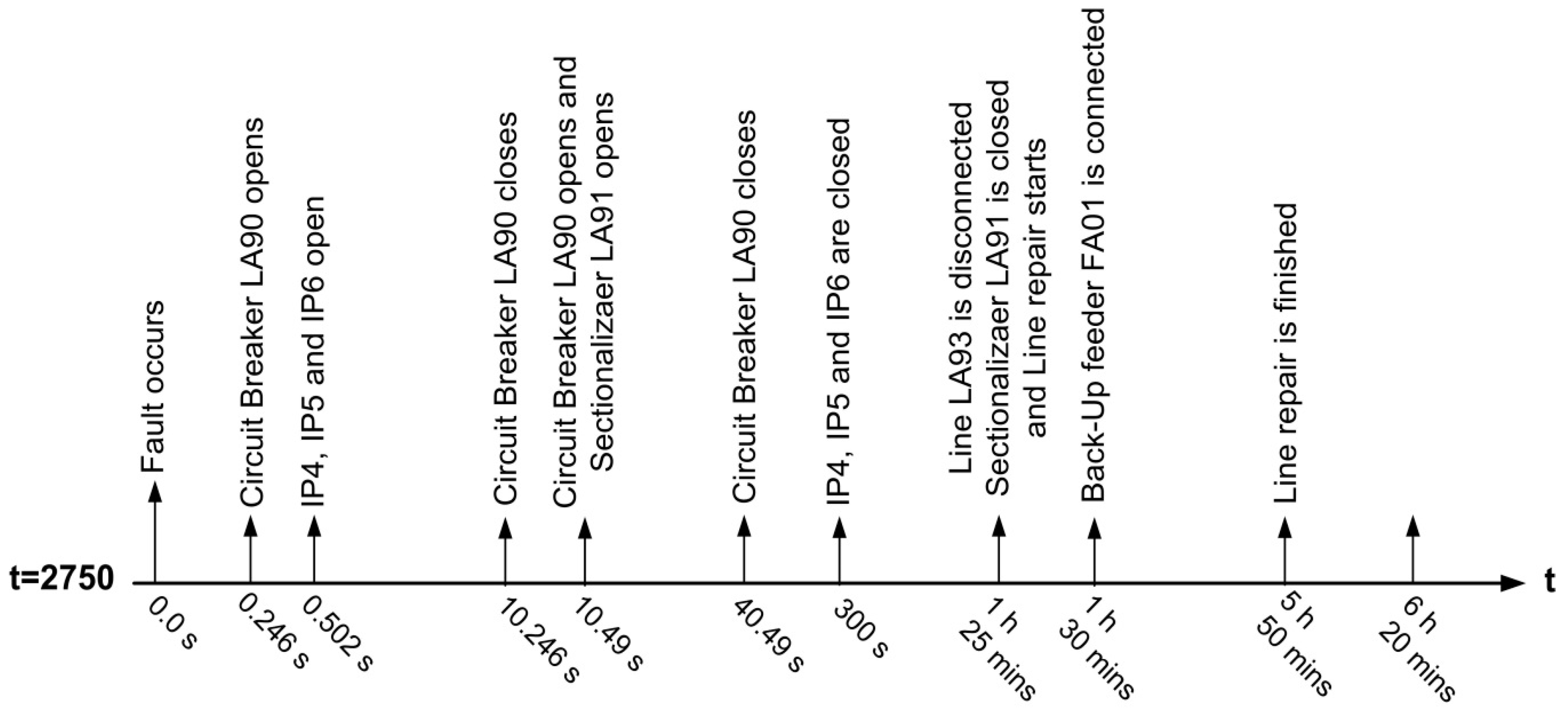
• Figure 5 provides a sequence of events with the time of occurrence of each event. As mentioned above, some of the values required to obtain this sequence are derived from the operation of the protective devices and are of deterministic nature, while others due to the performance of the maintenance crew are of random nature and generated according to the estimated probability distributions, see Section 6.
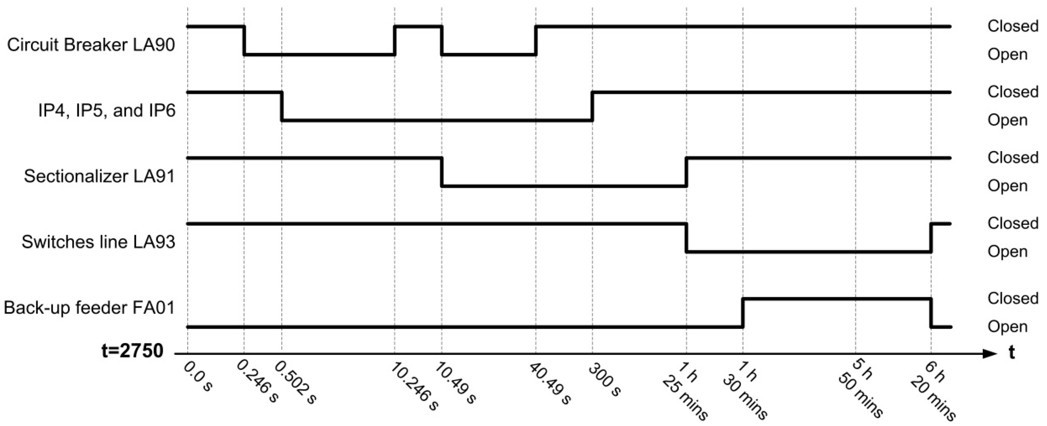
• Figure 6 shows a diagram with the status (e.g., opened/closed) of the protective devices and switches/disconnectors involved in this case.

5.4. Simulation Results

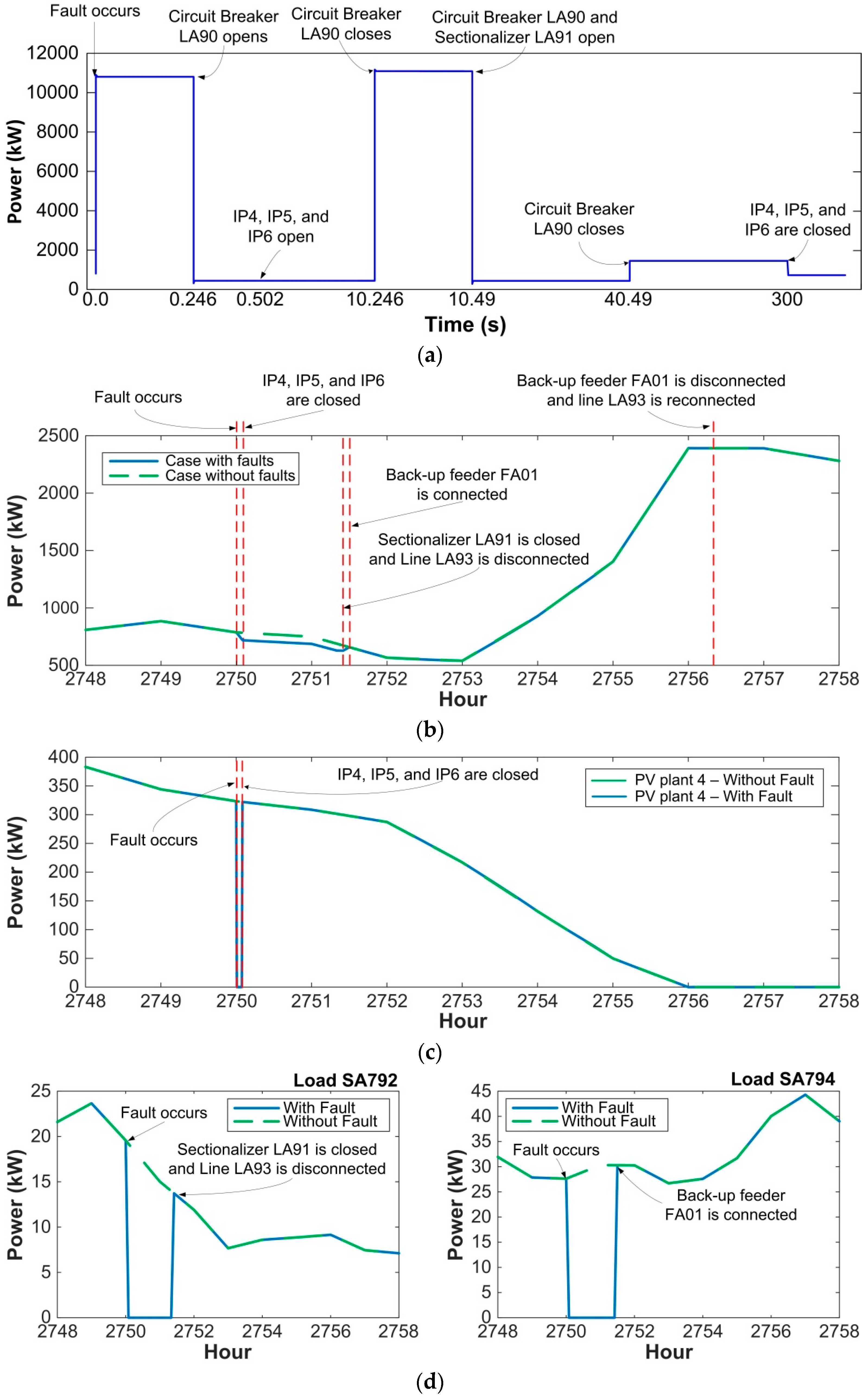
Figure 7 presents some results derived from the simulation of this case study. Note that, except for the first one, the plots have their time scale in hours, and they compare the power curves that result without the fault with those that are a consequence of the fault. The figures also incorporate some information about the operation of protective devices and switching operations.

Figure 7a presents the power provided from the high-voltage (HV) system. Power value exhibits a sudden increase when the fault occurs and remains approximately constant until circuit breaker LA90 performs the first opening action. Interconnection protections (i.e., IP4, IP5, and IP6) trip due to a low voltage condition at their PCCs; power values are not affected by this action since the entire feeder was previously isolated by circuit breaker LA90. The remaining value corresponds to the loads connected to the unfaulted feeder. Since the fault is still present after circuit breaker reclosing, a second opening operation is forced. This operation causes the sectionalizer LA91 to reach its count limit and open; as a consequence the circuit breaker will no longer sense any fault current. PV generators will be reconnected to the system after a normal voltage value has been confirmed at their PCCs. This action will cause a decrease in the power supplied from the HV system. Figure 7b presents the power supplied by the HV system during the complete simulation process: after the protection system has finished its operation sequence and the PV generators have been reconnected, a decrease in power can be observed when compared to pre-fault values. This decrease is a consequence of the loads disconnected by the operation of sectionalizer LA91. The procedure takes into account the time needed for the maintenance crew to reach the faulted line, isolate it, and return the sectionalizer to its original closed position. This sequence allows restoring service to all loads located upstream from the faulted line. The procedure also takes into account the time needed to perform load transfer when it is possible. For the present case, service can be restored to all loads downstream from the faulted line through the connection of a back-up feeder. Figure 7b shows how, after these two actions have been completed, service is restored to all loads in the system. Switching actions aimed at returning the system to its original state (i.e., reconnecting Line LA93 and disconnecting back-up feeder) are performed simultaneously and their effect on the system is neglected.

As mentioned above, the affected generators (i.e., PVplant4, PVplant5, and PVplant6) are separated from the system by their interconnection protection due to low voltage at their PCCs. Since no damage to the generators is assumed during the fault, they can be put back in operation as soon as possible; therefore, all tripped generators are reconnected after confirming normal voltage values at their PCCs. For the present case, those PV generators are located outside of the sectionalizer’s protection area and can be reconnected after the operation of the protection system; as a consequence, their downtime is very short, and the interruption can be considered momentary. Figure 7c presents the actual PVplant4 generation curve.

As a consequence of the sectionalizer operation, only loads SA792, SA794, and SA795 will suffer a sustained interruption. Load SA792 is located upstream the fault location and its service can be restored after isolating the faulted line and closing the sectionalizer; whereas loads SA794 and SA795 will remain without service until back-up feeder switch FA01 is connected. Figure 7d shows the power supplied to loads SA792 and SA794.

6. Studies and Results

This section details the different scenarios proposed in this paper for reliability analysis, presents the load- and generation-related reliability indices that will be calculated, and discusses the main simulation results. The positive impact that distributed generation (namely, PV generation) can have under some operating conditions is also discussed.

6.1. Reliability Studies

Three different scenarios have been considered to calculate reliability indices with and without distributed generation [5]:

• Only protective devices operate; that is, a protection device locks out after a permanent fault, and service is not restored before the faulted component is repaired.
• Switching operations aimed at isolating the faulted section are performed; this may restore service only to load nodes upstream the failed component.
• System reconfiguration may be used by means of transfer switches between feeders to restore service to some load nodes downstream the faulted section, depending on the system design.

The calculations are carried out with a time step of 1 h, but it is reduced when the fault/failure occurs since a shorter time step is required by protective device models in case of system fault. For more details about the time step size used in each interval from the moment at which the fault occurs until the moment at which the normal operation of the system is restored see [5].

According to IEEE Std 1366-2012 there exist a distinction between momentary and sustained interruptions [31]. On the other hand, faults/failures may be classified as temporary or permanent.

Although temporary distribution faults rarely exceed 5 min, depending on the grounding system design, it is possible to find longer temporary faults; therefore, momentary interruption (i.e., less than 5 min) should not be always seen as equivalent of temporary fault/failure (i.e., more than 5 min). A failure in an overhead line may be temporary or permanent, while a failure in any other component will be by default permanent. Finally, all faults are assumed by default bolted.

6.2. Some Remarks

• Network reconfiguration and surplus in PV generation can cause reverse power flow through voltage regulators. Reverse power flow can interfere with voltage regulator control and cause unacceptable operating conditions; therefore, voltage regulator control will be disabled during reverse power flow.
• A fault in a line section close to the substation will cause a voltage dip at the nodes of the adjacent feeder, and this could cause the operation of the undervoltage protection of PV generators. Protective devices have been coordinated to avoid these consequences; that is, the overcurrent relay installed to protect the faulted feeder will be faster that the undervoltage protection of PV generators connected to the adjacent feeder.
• Load transfer will be carried out only when normal operating conditions are ensured. That is, when load transfer is considered, the procedure will be as follows: (1) check for availability of back-up feeder; (2) if there is an available back-up feeder, load is transferred; (3) during the simulation, voltages at load points and phase currents through lines and voltage regulators are monitored; (4) when the simulation is finished, the procedure checks for the technical restrictions (all load point voltages are above 0.9 pu; phase current through distribution lines and voltage regulators do not exceed 110% of nominal rating); (5) if one of the previous restrictions is not satisfied the procedure will deem the operation not successful and repeat the simulation without considering load transfer.
• Some special situations have to be considered; one of these situations can occur when load transfer is possible and two maintenance crews are involved: one will take care of the repair and associated operations (e.g., isolation of the failed component), the other one will take care of the transfer maneuver. Both actions are considered independent from each other, and the moments at which the repair of the failed component will finish and the transfer maneuver will be made are randomly estimated. As a consequence of these calculations, the transfer maneuver should be made prior to the moment at which the other crew would finish the repair; if the time interval between the two moments is shorter than 15 min then the transfer operation is not carried out to avoid that an additional maneuver had to be made short after the failed component was repaired.
• A different situation can occur with the previous scenario if some remote control and small values are assumed for some switching times. Remember that back-up feeder connection time is randomly generated and follows an exponential distribution. Two cases have been considered:

  -

  Back-up feeder connection time is shorter than the time needed to disconnect the failed element and close the operated protective device: in this case the procedure will perform both actions simultaneously, using the longer time for both actions.

  -

  Back-up feeder connection time is longer than the time needed to disconnect the failed element and close the operated protective device: for this condition the procedure will perform both actions independently at their specified times.

• If a one-phase fault occurs on a distribution line protected by a fuse, two cases can be considered:

  -

  Phase voltages at LV load points are above 0.9 pu: the repair will be carried out in a normal manner; loads will not experience any interruption.

  -

  Phase voltages at LV load points are below 0.9 pu: the healthy phases will then be opened, isolating all elements downstream from the operated fuse.

  If a two-phase fault occurs on a distribution line protected by a fuse, the remaining phase must be opened to disconnect all voltage sources from the failed zone.

6.3. Reliability Indices

To assess the impact of DG on the distribution system reliability, the calculations presented in this paper compare the indices that result from the three scenarios with and without generation; however, for a better assessment the indices when PV generation units are connected to the test system have also been calculated assuming that the generation equipment (i.e., PV modules and interconnection transformers) never fails.

In addition to the classical distribution reliability indices [31], the following two additional indices related to power generation, and named according to [12], have been estimated:

• System Average Interruption Frequency Index for DG (SAIFI_DG):

  $$SAIF{I}_{DG}=\frac{{\displaystyle \sum _{i=1}^{k}P{G}_i}}{P{G}_T}$$

  (1)
• System Average Interruption Duration Index for DG (SAIDI_DG):

  $$SAID{I}_{DG}=\frac{{\displaystyle \sum _{i=1}^{k}P{G}_i}\cdot H_i}{P{G}_T}$$

  (2)

  where k is the number of sustained interruptions in the distribution system corresponding to a given year, PG_i is the number of rated kWs of PV generation disconnected from the system during an interruption in the system, PG_T is the total rated generation, measured in kW, and H_i is the duration of the disconnection for the PV generation affected by the interruption.

The index SAIFI_DG is the average number of interruptions that each kW of rated generation experiences, while the index SAIDI_DG is the average outage duration for each kW of rated generation.

A third index is the Actual Energy Not Produced (AENP). It is the difference between the actual energy produced when the system is simulated without any fault (i.e., base case) and that resulting when faults can occur.

6.4. Simulation Results

The calculation of probability density functions of reliability indices is made using a distributed computing environment with 60 cores, see Figure 1. The stopping criterion used for assessing convergence is the coefficient of variation (CV) [5], which helps to determine if enough executions have been performed in order to estimate the probability density function (PDF) of a variable. In this paper, it is assumed that the Monte Carlo method has converged when the CV of all calculated indices is below 5%.

Table 3. Reliability Indices—Sensitivity Study.

Index		Without DG	With DG (DG Equipment Does Not Fail)		With DG (DG Equipment Can Fail)
		360 runs	360 runs	420 runs	360 runs	420 runs
SAIFI (int)	Mean	1.203	1.203	1.1723	1.197	1.163
	Deviation	0.612	0.612	0.654	0.607	0.613
	CV (%)	2.680	2.6796	2.720	2.672	2.569
SAIDI (h/year)	Mean	2.703	2.641	2.596	2.676	2.587
	Deviation	1.375	1.285	1.280	1.426	1.373
	CV (%)	2.681	2.564	2.406	2.809	2.590
CAIDI * (h/int)	Mean	2.683	2.638	2.809	2.699	2.628
	Deviation	1.711	1.696	1.896	1.819	1.537
	CV (%)	3.362	3.388	3.293	3.553	2.854
AENS (kWh/year)	Mean	8592.6	8365.6	8266.3	8565.6	8186.9
	Deviation	4730.4	4354.3	4475.9	4976.6	4668.5
	CV (%)	2.901	2.743	2.642	3.062	2.782
SAIFIDG (int)	Mean		1.108	1.078	1.361	1.327
	Deviation	-----	0.658	0.697	0.696	0.684
	CV (%)		3.130	3.157	2.695	2.515
SAIDIDG (h/year)	Mean		1.659	1.634	6.212	6.057
	Deviation	-----	1.500	1.571	5.984	5.240
	CV (%)		4.763	4.692	5.077	4.221
AENP (kWh/year)	Mean		489.4	486.3	1837.3	1883.8
	Deviation	-----	593.2	613.5	2092.3	1908.7
	CV (%)		6.389	6.155	6.002	4.944

* CAIDI stands for Customer Average Interruption Duration Index [31].

shows the values obtained for some reliability indices derived after 360 and 420 runs, and considering only Scenario 3 (see Section 6.1). According to the results provided in Table 3, 360 runs are enough to estimate load-related reliability indices with enough accuracy. However, the CV value after 360 runs is more than 5% for those indices related to generation; the main reason is the low number of generation units that are affected by a fault. Reliability indices are calculated as recommended by IEEE Std 1366 [31] or according to the above expressions. The acronym AENS stands for Actual Energy Not Supplied, and was introduced in [5].

Table 4. Probability Distributions of Reliability Indices—420 runs.

Scenario	Index	Without DG		With DG (DG Equipment Does Not Fail)		With DG (DG Equipment Can Fail)
		Mean	Deviation	Mean	Deviation	Mean	Deviation
1—Service is restored to affected customers after repair	SAIFI (int)	1.205	0.652	1.205	0.652	1.200	0.612
	SAIDI (h/year)	5.522	3.170	5.522	3.170	5.689	3.302
	CAIDI (h/int)	5.074	2.307	5.074	2.307	5.007	2.189
	AENS (kWh/year)	17529.2	10179.6	17529.1	10179.6	17887.7	10456.7
	SAIFIDG (int)	-----	-----	1.078	0.697	1.327	0.684
	SAIDIDG (h/year)	-----	-----	4.640	3.946	9.325	6.246
	AENP (kWh/year)	-----	-----	1464.1	1713.7	2971.9	2620.4
2—Service is restored to some customers after switching	SAIFI (int)	1.176	0.654	1.176	0.654	1.167	0.613
	SAIDI (h/year)	3.778	2.396	3.778	2.396	3.936	2.569
	CAIDI (h/int)	3.809	2.441	3.809	2.441	3.741	2.216
	AENS (kWh/year)	11698.2	7232.8	11698.2	7232.8	12122.0	7722.2
	SAIFIDG (int)	-----	-----	1.078	0.697	1.327	0.684
	SAIDIDG (h/year)	-----	-----	3.256	3.319	7.900	5.862
	AENP (kWh/year)	-----	-----	1043.2	1375.4	2486.9	2310.8
3—Service is restored to some customers after reconfiguration	SAIFI (int)	1.173	0.654	1.173	0.654	1.163	0.613
	SAIDI (h/year)	2.654	1.316	2.596	1.280	2.587	1.373
	CAIDI (h/int)	2.861	1.909	2.809	1.896	2.628	1.537
	AENS (kWh/year)	8475.2	4631.5	8266.3	4475.9	8187.0	4668.5
	SAIFIDG (int)	-----	-----	1.078	0.697	1.327	0.684
	SAIDIDG (h/year)	-----	-----	1.634	1.571	6.057	5.240
	AENP (kWh/year)	-----	-----	486.3	613.5	1883.8	1908.7

shows the results obtained for the three scenarios. Given the results presented in Table 3, the number of runs considered without and with DG has been 420. Table 4 presents a summary of the probability distributions of these indices.

Table 5. Simulation Times—Scenario 3.

Reliability Study		Runs	1 core	60 cores
Base case with Distributed Generation		1 run	191 s	-
Without Distributed Generation		1 run	5256 s	-
		360 runs	-	38237 s
With Distributed Generation	DG equipment does not fail	1 run	5375 s	-
	DG equipment can fail	1 run	5427 s	-
	DG equipment does not fail	420 runs	-	45405 s
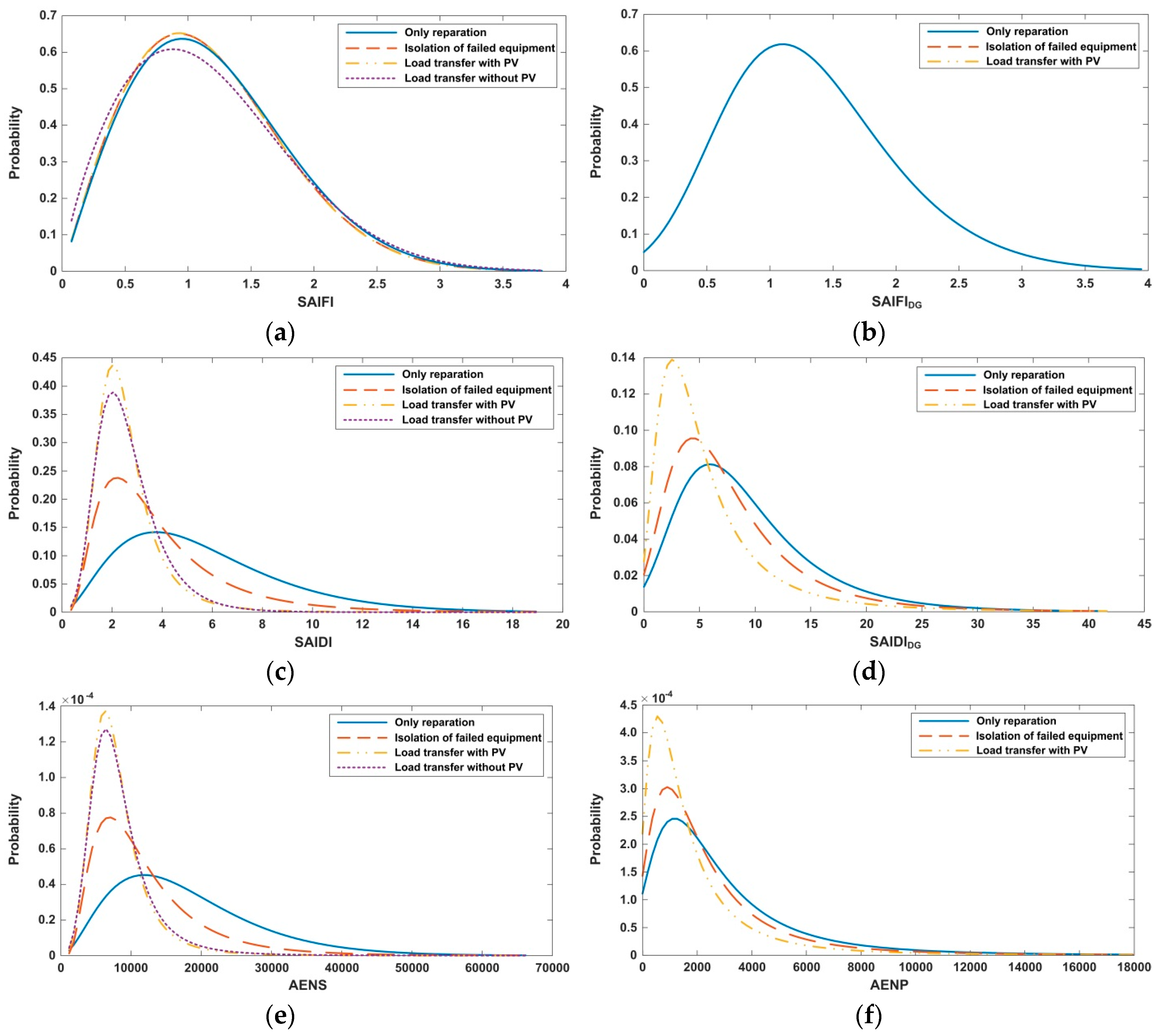
	DG equipment can fail	420 runs	-	46154 s

provides the computing time that was needed for the options considered with Scenario 3, which is the most sophisticated one and for which the longest simulation times are required. The probability density functions for some reliability indices are shown in Figure 8.

Load Indices: The restrictions upon the formation of islands causes load indices to present similar probability distributions with and without PV generation. Note that the SAIFI (System Average Interruption Frequency Index) index, which depends only on failure rates, is very similar in all studies. The differences are basically due to single-phase faults: when a single-phase fault provokes a fuse operation, affected loads may suffer a voltage drop instead of an interruption. Scenario 1 presents higher values for this index: as previously explained, every time a one-phase fault occurs, the system checks the minimum voltage at load terminals; if the minimum voltage is below 0.9 pu, the procedure will open the remaining phases, causing an interruption to all loads downstream from the operated fuse. Finally, Scenario 2 presents values slightly higher than Scenario 3 but lower than Scenario 1; single-phase faults protected by fuses are again responsible for this behaviour. As in Scenario 1, the procedure checks the minimum voltage at load terminals; if the minimum voltage is below 0.9 pu, then the failed line will be isolated and the operated fuse replaced. Under these circumstances only load downstream from the failed line will suffer a sustained interruption. If load transfer through a back-up feeder is possible (i.e., Scenario 3) and the connection time is lower than the time required to isolate the failed line and replace the operated fuse, the procedure will perform both actions simultaneously; as a consequence loads located downstream from the failed line will not experience any sustained interruption. The differences between SAIDI (System Average Interruption Duration Index) values for Scenarios 1 and 2 are clear: the possibility of isolating the failed element and closing the operated protection device reduces the interruption time experienced by loads upstream from the failed element, having this decrease an impact on the global SAIDI value. Moreover, the possibility of load transfer, which allows quickly restoring service to those loads located downstream from the failed element, will further reduce the index. As for AENS, the conclusions are similar to those drawn for SAIDI.

DG Indices: The results provided in Table 4 show that SAIFI_DG values are the same for all 3 scenarios, while SAIDI_DG values depend on the level of automation (i.e., the scenario under study). These results are reasonable since all protective devices between PV generators and the substation transformer are three-phase and the number of interruptions does not depend on the automation incorporated to the system. However, the SAIDI_DG reduction is lower when compared to load indices because the failure of DG equipment is independent from network automation level and normal operation can only be resumed after all repairs have been finished. As for AENP, its variation is similar to that obtained for SAIDI_DG.

6.5. Simulation Time

The minimum simulation time required for reliability assessment with the approach presented in this work would be approximately the time required for a single run if the number of runs and the number of cores are equal. However, both the number of runs and the simulation time would be much higher if the procedure had to be applied to a larger system (e.g., several hundreds of nodes). The computing times presented in Table 5 correspond to the complete simulation of the test system during a year; however, as shown in [5], a significant reduction of the simulation time without affecting reliability index accuracy can be achieved by simulating the system only when sustained interruptions are caused. Therefore, a significant reduction in simulation time is still possible; the quantities presented here should be seen as the upper limit of simulation time when reliability assessment is based on the application of a power flow simulator.

7. Impact of Distributed Generation on Distribution System Reliability

The main goal of this paper is to propose a procedure that could be used for reliability analysis of distribution systems with and without DG and considering different levels of automation. The results presented in Table 3 and Table 4 correspond to the study of the test system under certain load and generation conditions. Therefore, the conclusions derived from those results should be used with care. Although the differences obtained for load indices are not too significant with and without DG, the fact is that DG can positively impact reliability even if islanding conditions (i.e., microgrids) are not allowed. This section is aimed at clarifying how and when this is possible.

First, remember that PV generation can only help during day-time hours when solar radiation is non-zero; this means that under some operating conditions its impact during that period of the day can be significant. Second, restrictions in operating conditions have to be considered in order to determine whether load transfer is possible or not.

Two case studies corresponding to two different failures on the test system with and without PV generation are analysed below.

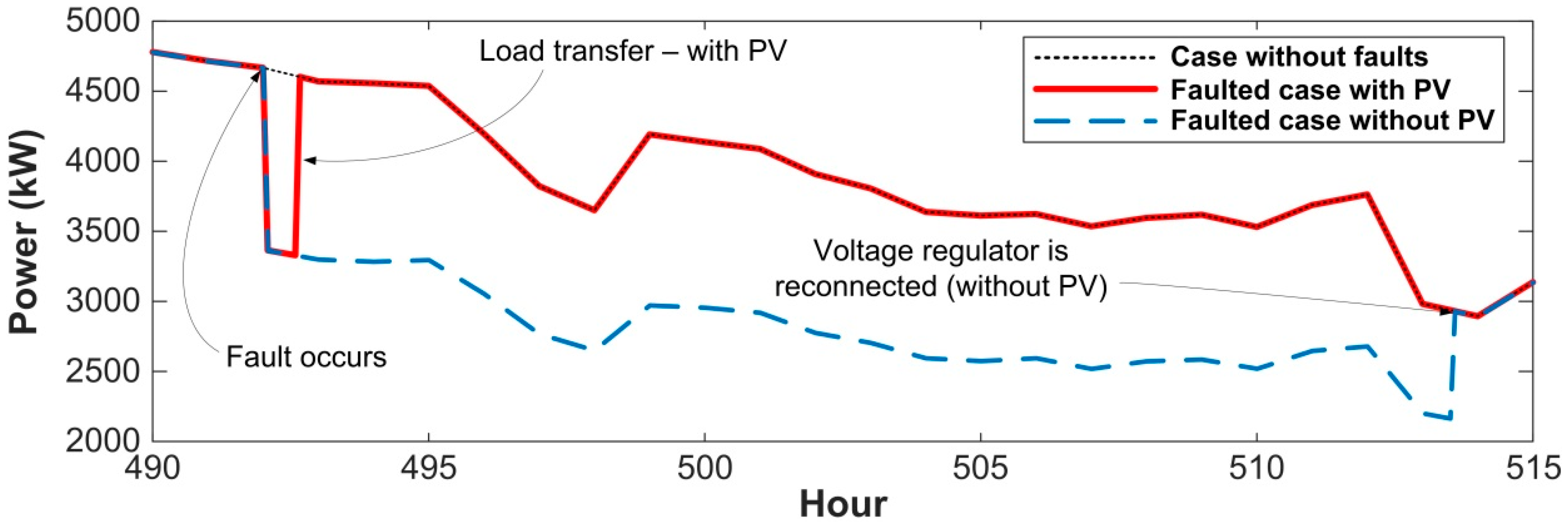
Figure 9 illustrates the impact of a three-phase failure in the voltage regulator located between nodes 743 and 747, see Figure 2. Given the location of the failed component, a load transfer using the intermediate switch transfer should be considered. However, since the failure occurs at noon of a January’s day, the presence of PV generators has a significant impact: without these generators, there would be an overload of the voltage regulator located on the right feeder, and load transfer is not made. As a consequence, service cannot be restored to all load nodes (about 3 MW of rated power) and the actual energy not supplied during service interruption reaches a value close to 23 MWh, see Figure 9.

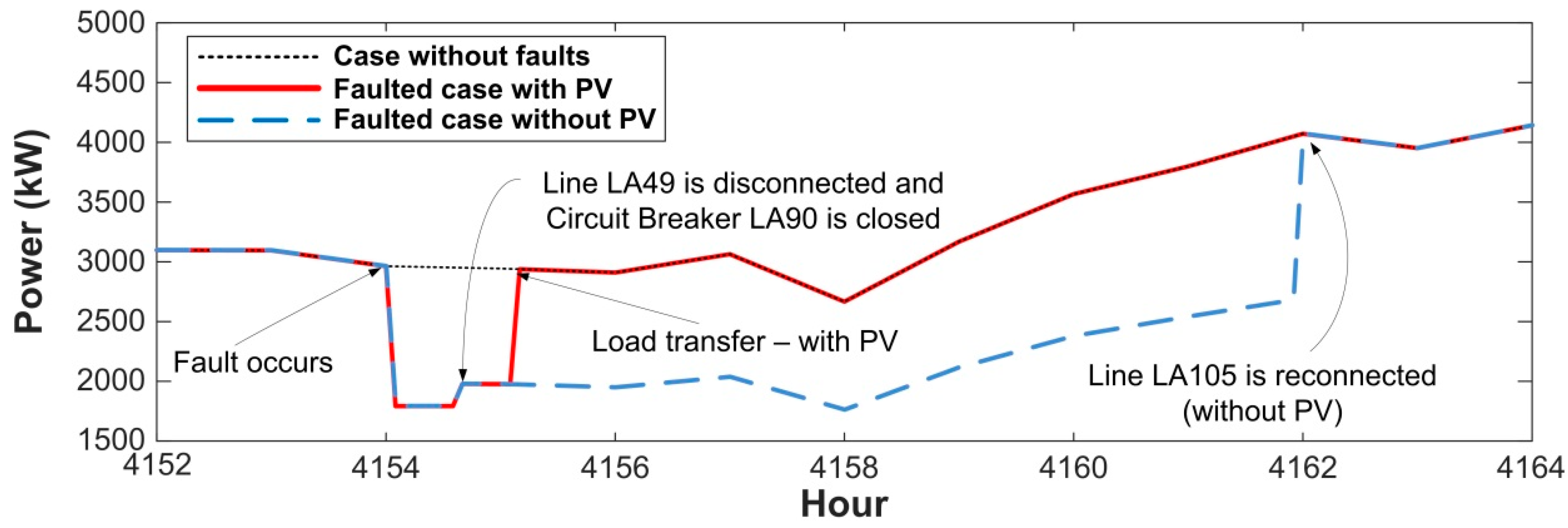
A similar case is presented in Figure 10: a one-phase fault occurs early in the morning (when PV generation is zero) in the line section located between nodes 803 and 805, see Figure 2. One more time, load transfer is not possible due to overload of a voltage regulator. Although the PV generation cannot initially affect the system operation because there is no solar radiation, due to the time required for repair and service restoration, solar generation becomes more important and can help the load transfer option, which would only be feasible with the presence of PV generation; see Figure 8.

An obvious conclusion can be derived from these two cases: if the load level was higher than that assumed in the previous study, the impact of PV generation would have been more significant than reflected in Table 3 and Table 4.

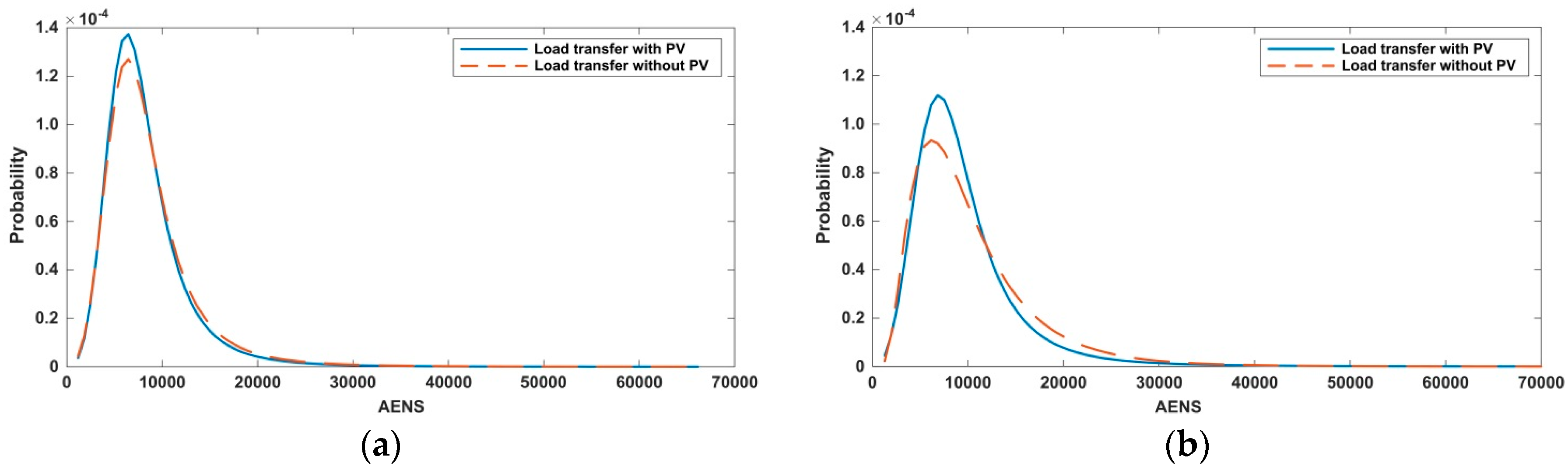
Figure 11 and

Table 6. Comparison of Reliability Indices. Scenario 3: Service is restored to some customers after reconfiguration—420 runs.

Index	Without DG		With DG (DG Equipment Does Not Fail)		With DG (DG Equipment Can Fail)
	Mean	Deviation	Mean	Deviation	Mean	Deviation
Initial operating conditions
SAIFI (int)	1.173	0.654	1.173	0.654	1.163	0.613
SAIDI (h/year)	2.654	1.316	2.596	1.280	2.587	1.373
CAIDI (h/int)	2.861	1.909	2.809	1.896	2.628	1.537
AENS (kWh/year)	8475.2	4631.5	8266.3	4475.9	8186.9	4668.5
SAIFIDG (int)	-----	-----	1.078	0.697	1.327	0.684
SAIDIDG (h/year)	-----	-----	1.634	1.571	6.057	5.240
AENP (kWh/year)	-----	-----	486.3	613.5	1883.8	1908.7
New operating conditions
SAIFI (int)	1.173	0.654	1.173	0.654	1.163	0.613
SAIDI (h/year)	2.970	1.785	2.721	1.418	2.796	1.612
CAIDI (h/int)	3.152	2.203	2.926	2.027	2.803	1.655
AENS (kWh/year)	10281.7	6423.4	9408.7	5378.1	9643.4	6023.5
SAIFIDG (int)	-----	-----	1.078	0.697	1.327	0.684
SAIDIDG (h/year)	-----	-----	1.801	1.786	6.344	5.283
AENP (kWh/year)	-----	-----	571.7	701.8	1907.5	1802.7

show the reliability indices that result with the initial and the new operating conditions, in which load profiles have been modified in order to produce a load increment during day-time hours without increasing load rated powers. Both studies were carried out considering Scenario 3. Under the new conditions, system reliability becomes more sensitive to PV generation and those indices related to interruption duration (SAIDI, CAIDI, and AENS) increase. Since PV generation can only provide support during day-time hours, PV generation can have a significant impact on system reliability if system loads are predominantly diurnal.

8. Discussion

When the service is restored after an outage, the demand is usually greater than before the outage. This phenomenon, referred to as cold load pickup, can affect the performance of some protective devices which can misinterpret the new condition as a fault, and initiate the de-energization of an unfaulted system. The factors that can affect the magnitude and duration of this phenomenon are many: outage duration, types of connected load, weather, restoration mode, outage causes, the presence of distributed generation and/or automatic transfer schemes, time of day, and load level. For a detailed discussion of this phenomenon and the above factors, see [32,33]. The impact of cold load pickup on reliability studies is usually neglected. Since load variation occurs after service restoration, the impact should also be quantified on the demanded power from the high voltage system and/or distributed generators. In addition, one can assume that at the time a new service interruption occurs the impact on the load level caused by the previous interruption has already disappeared. As mentioned above, the impact of this phenomenon is higher at the time service is restored since overcurrent conditions can be generated due to inrush currents; a deep analysis of these conditions is out of the scope of this work since a different simulation tool (e.g., an EMTP-like tool) would be required.

However, another approach can be applied if it is assumed that the transients caused during service restoration will not be dangerous for system components, and there will be no misoperation of protective devices. Under such assumption, the cold load pickup phenomenon can be included by considering an extended load model; that is, load profiles should be expanded for including the load variation to be considered at any time of the day in case of interruption, irrespective of its duration (i.e., momentary or sustained).

9. Conclusions

This paper has presented a procedure based on a Monte Carlo method for reliability assessment of overhead distribution systems with or without distributed generation using a multicore computing environment and a power flow simulator running in time-driven mode. This approach offers some important advantages (see also [5]): (1) the model can be realistic and detailed, and results can be very accurate; (2) simulation results provide a significant amount of information that can be used for other purposes (e.g., optimum location of DG units); (3) the information can also be used for estimating other performance indices than those presented here.

It is evident from the results presented in this paper, that although the use of a multicore computing environment can reduce the simulation time to approximately that corresponding to a single run with an adequate number of cores, this could be possible for large systems only when a much higher number of cores was available.

Although the main goal of the paper is to propose a procedure for reliability analysis, the results presented here prove that, depending on the operating conditions, distributed generation can improve the reliability of distribution systems, mainly due to the overload that could occur in a faulted system without the presence of embedded generation; this is especially important when load transfer between feeders is possible in the system under study.

The present work has been carried out with a detailed distribution system model but with several limitations (e.g., PV units inject only active power; DG is not used to control voltages of distribution system nodes). Future work should be addressed to solve aspects that could be important for an accurate analysis of the smart grid: a shorter time step should be used to cope with fast variations of PV generation; PV generation could inject/absorb reactive power; DG could be used to control the voltage of distribution system nodes; load profiles should be edited to cope with the phenomenon of the cold load pickup; more detailed models for reliability analysis, mainly for some DG technologies, could be used; islanding conditions should be allowed by incorporating microgrids to the distribution system. Note that some of these items imply much more powerful simulation tools.