
State Estimation of Permanent Magnet Synchronous Motor Using Improved Square Root UKF

Abstract
:1. Introduction
2. Square-Root UKF
2.1. The Minimal Skew Simplex Points
- (1)
- Choose the initial weight value:
- (2)
- Choose weight sequence:
- (3)
- Initialize the vector sequences of sigma points as:
- (4)
- Expand vector sequences for j = 2,…,n, according to:
2.2. Square-Root UKF for State-Estimation
- (1)
- Initialize withwhere denotes an initial guess for the initial state , and is the initial estimation variance. Chol (·) represents the matrix square-root using lower triangle Cholesky decomposition.
- (2)
- Sigma point calculation and time updatewhere qr{·} and cholupdate{·} represents QR decomposition and Cholesky factor updating.
- (3)
- Measurement update
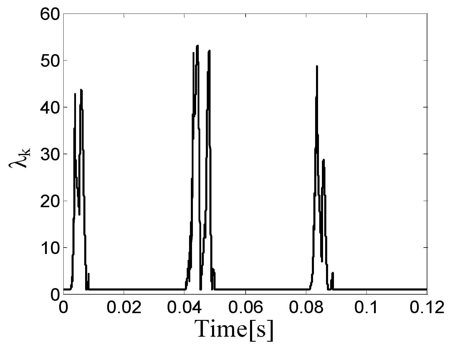
3. Improved SRUKF
4. Mathematical Model of PMSM and System Implementation
4.1. Mathematical Model of PMSM
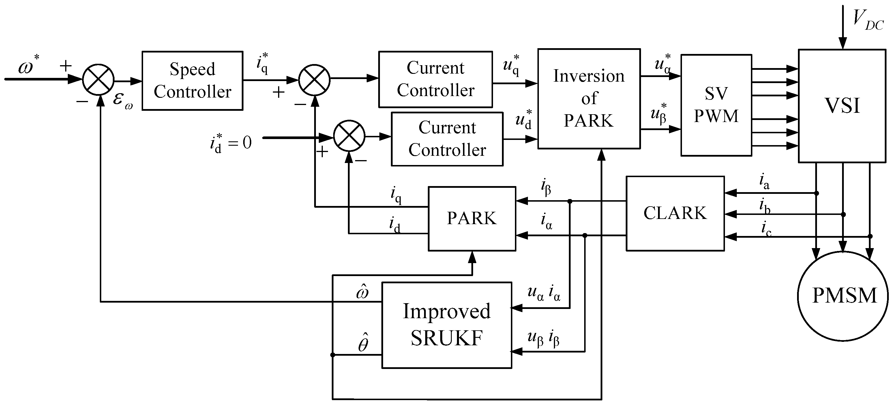
4.2. System Implementation
5. Simulation Results and Error Analysis
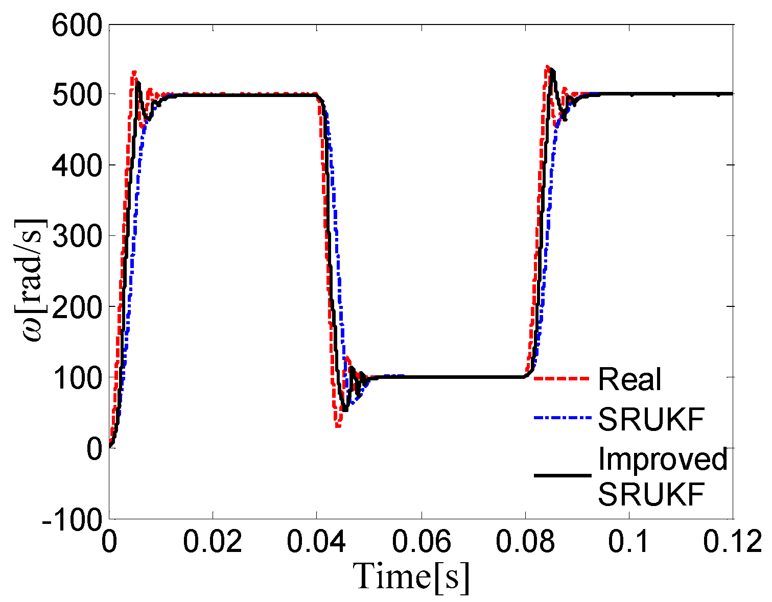
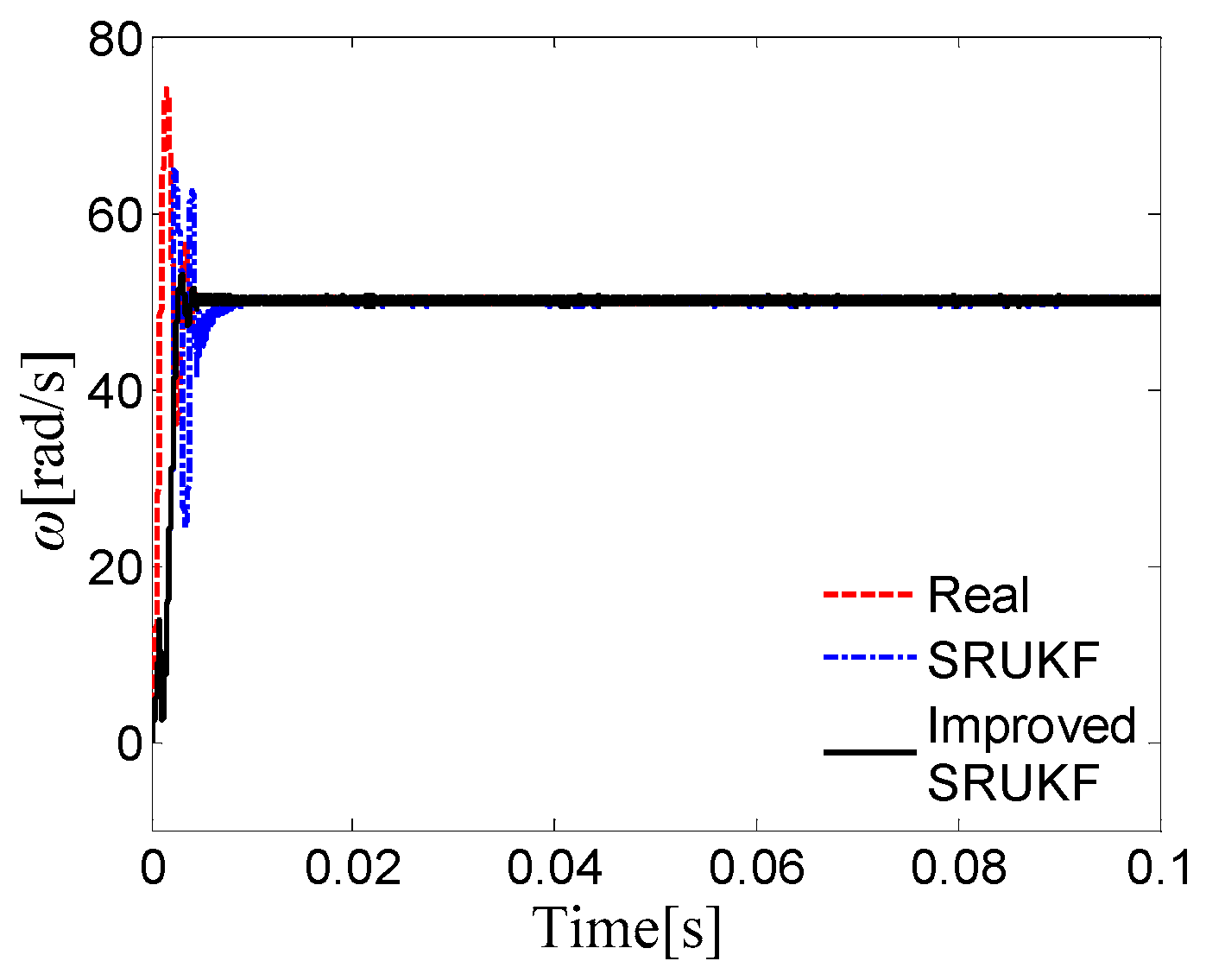
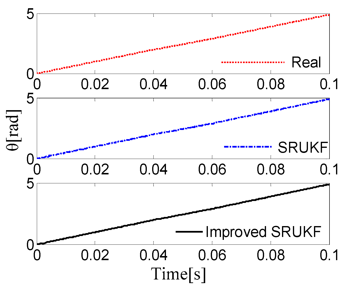
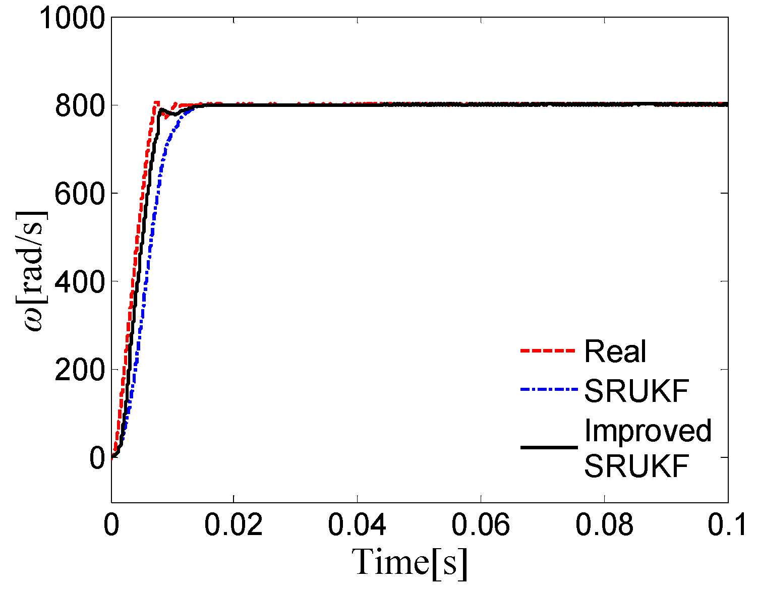
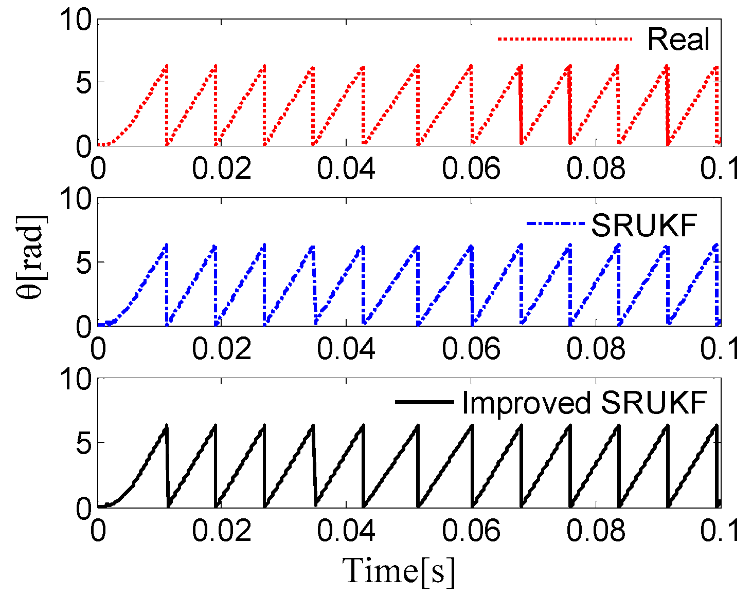
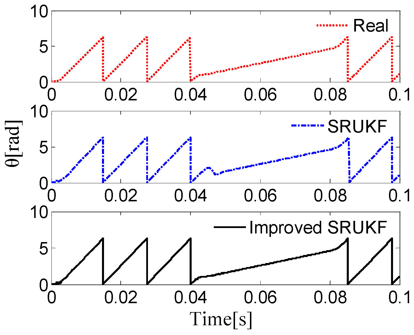
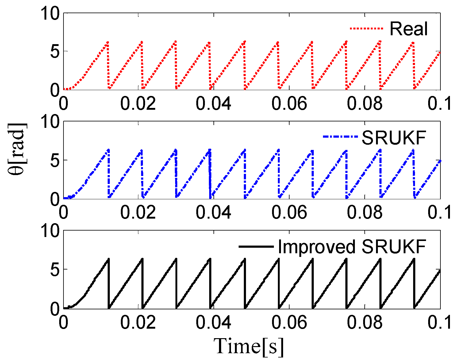
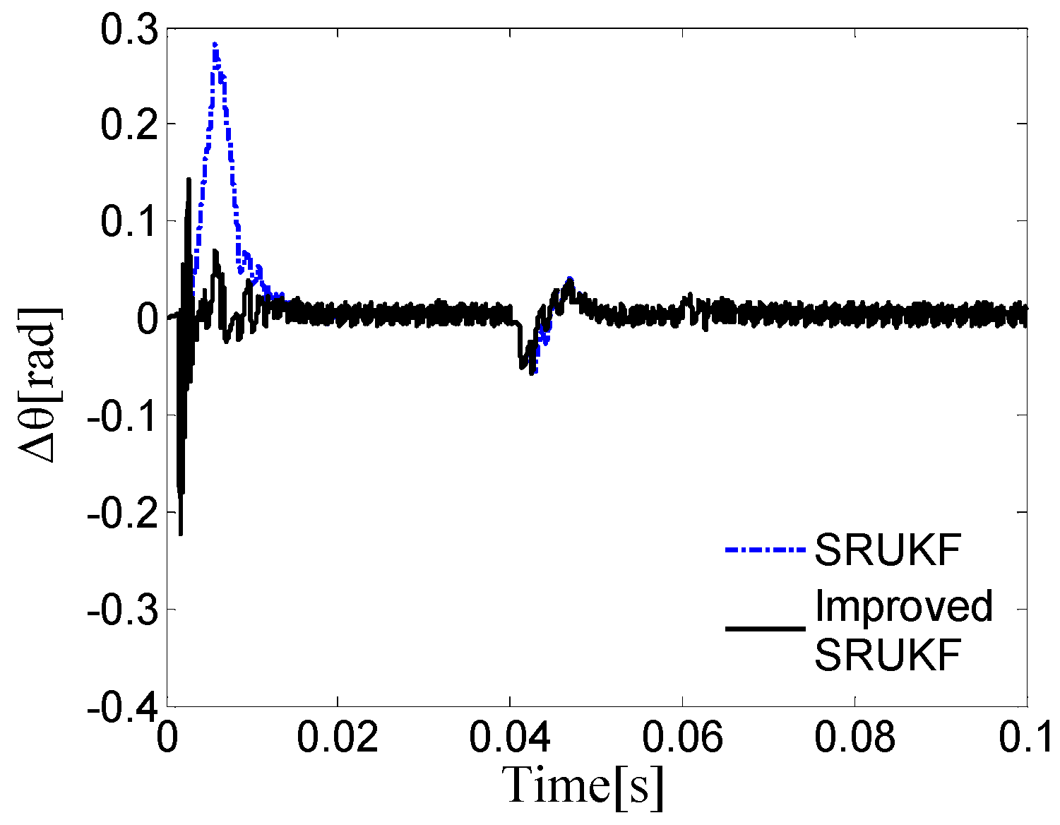
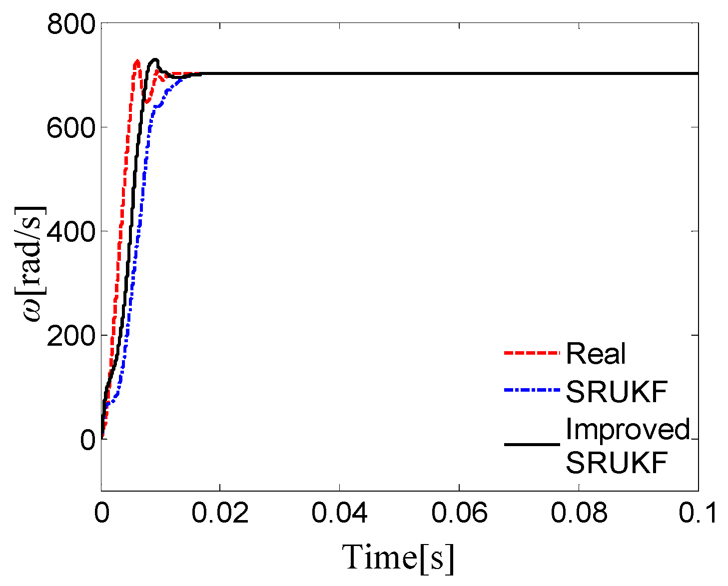
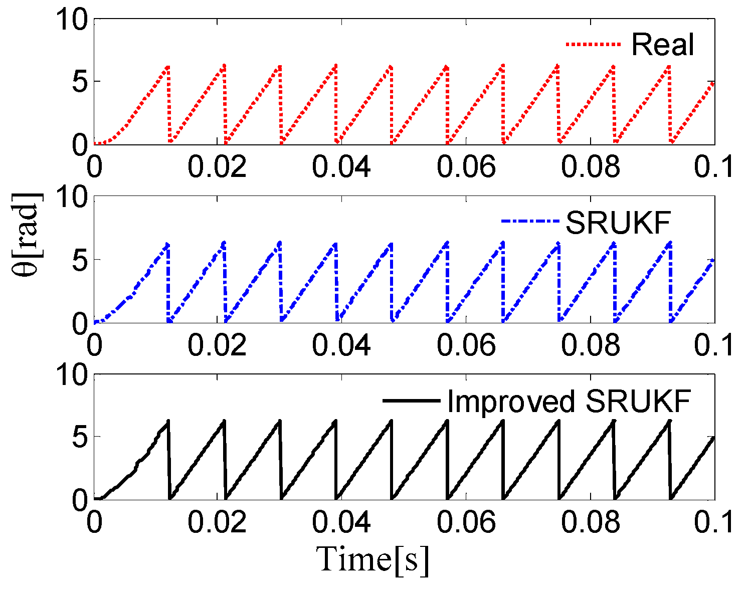
5.1. Simulation Results
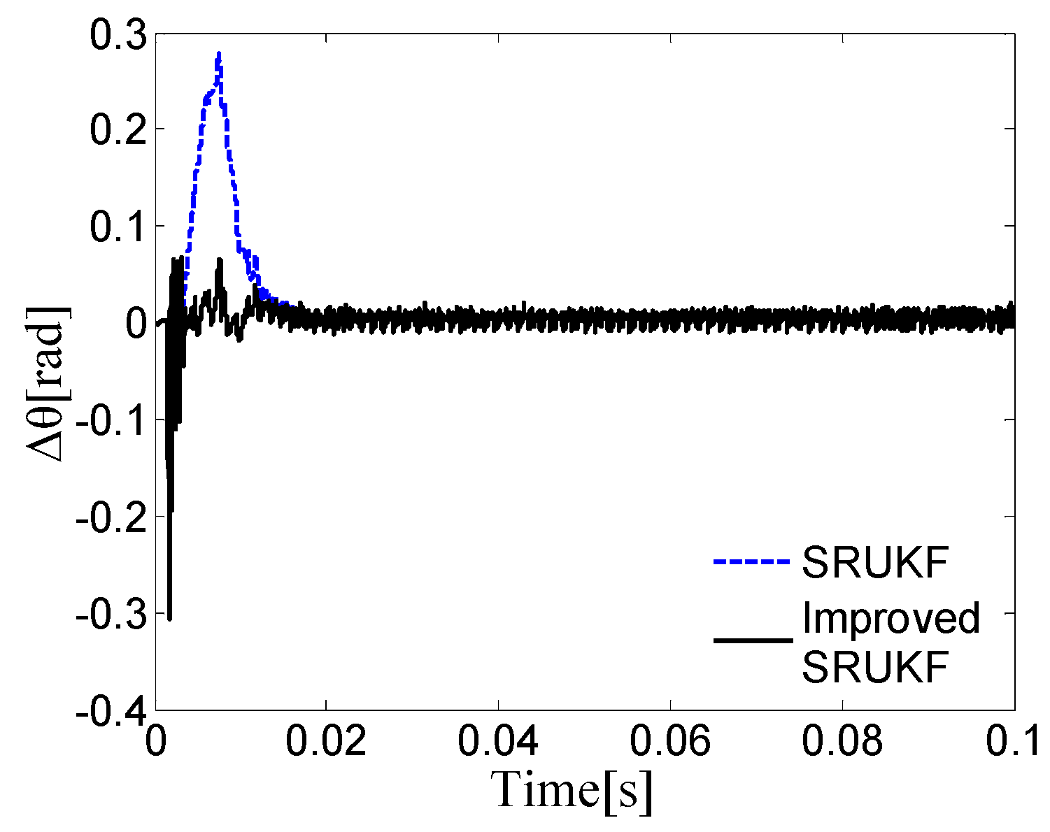
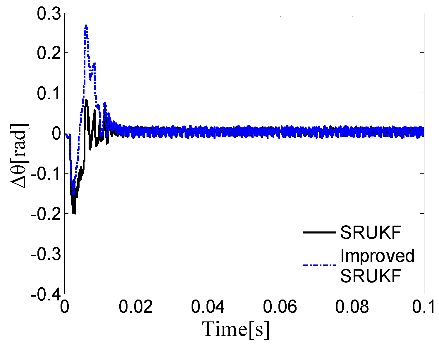
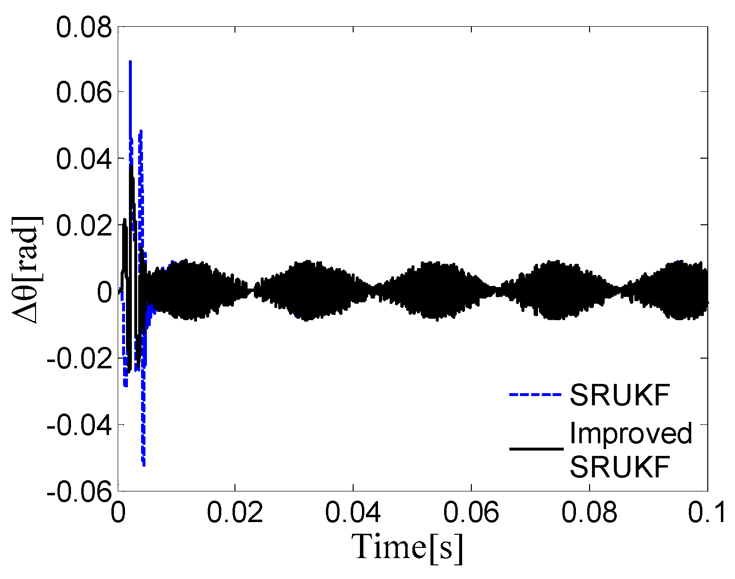
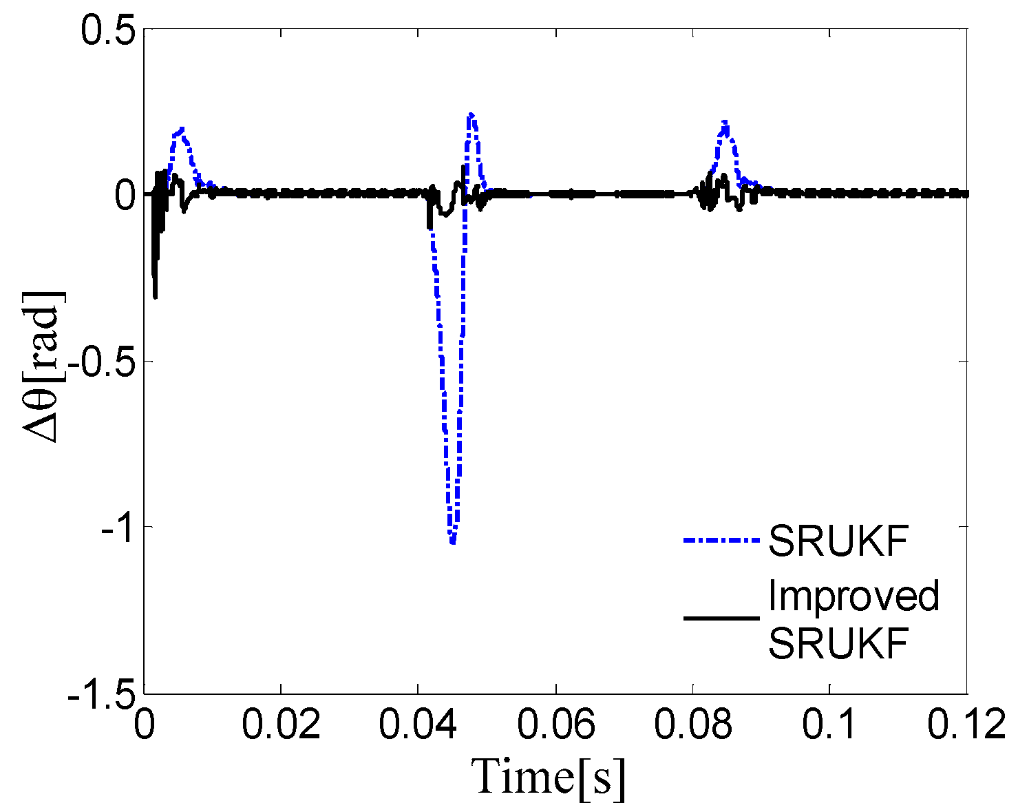
5.2. Error Analysis
6. Conclusions
Acknowledgments
Author Contributions
Conflicts of Interest
Nomenclature
| P1 | Number of poles pairs in torque winding |
| R | Stator resistance |
| Ld (Lq) | Stator inductance in d–q coordinate system |
| ψf | Magnet flux linkage |
| J | Rotor moment of inertia |
| M | Rotor mass |
| V | Rated voltage of torque winding |
| I | Rated current |
| Te | Electromagnetic torque |
| T | Mechanical time constant |
| Tm | Rated mechanical torque |
| Ts | Sampling period |
| θ | Rotor angle position |
| ω | Rotor speed |
| F | Friction coefficient |
| uα (uβ) | Stator voltage in α–β coordinate system |
| iα (iβ) | Stator current in α–β coordinate system |
References
- Kalman, R.E. A new approach to linear filtering and prediction problems. J. Basic Eng. 1960, 82, 35–45. [Google Scholar] [CrossRef]
- Alonge, F.; D’Ippolito, F.; Sferlazza, A. Sensorless control of induction-motor drive based on robust Kalman filter and adaptive speed estimation. IEEE Trans. Ind. Electron. 2014, 61, 1444–1453. [Google Scholar] [CrossRef]
- Salvatore, N.; Caponio, A.; Neri, F.; Stasi, S.; Cascella, G.L. Optimization of delayed-state Kalman-filter-based algorithm via differential evolution for sensorless control of induction motors. IEEE Trans. Ind. Electron. 2010, 57, 385–394. [Google Scholar] [CrossRef]
- Masi, A.; Butcher, M.; Martino, M.; Picatos, R. An application of the extended Kalman filter for a sensorless stepper motor drive working with long cables. IEEE Trans. Ind. Electron. 2012, 59, 4217–4225. [Google Scholar] [CrossRef]
- Laamari, Y.; Chafaa, K.; Athamena, B. Particle swarm optimization of an extended Kalman filter for speed and rotor flux estimation of an induction motor drive. Electr. Eng. 2015, 97, 129–138. [Google Scholar] [CrossRef]
- Bolognani, S.; Oboe, R.; Zigliotto, M. Sensorless full-digital PMSM drive with EKF estimation of speed and rotor position. IEEE Trans. Ind. Electron. 1999, 46, 184–191. [Google Scholar] [CrossRef]
- Lu, K.Y.; Lei, X.; Blaabjerg, F. Artificial inductance concept to compensate nonlinear inductance effects in the back EMF-based sensorless control method for PMSM. IEEE Trans. Energy Convers. 2013, 28, 593–600. [Google Scholar] [CrossRef]
- Kumar, S.; Prakash, J.; Kanagasabapathy, P. A critical evaluation and experimental verification of Extended Kalman Filter, Unscented Kalman Filter and Neural State Filter for state estimation of three phase induction motor. Appl. Soft Comput. 2011, 11, 3199–3208. [Google Scholar] [CrossRef]
- Julier, J.S.; Uhlmann, J.; Whyte, H.D. A new method for the nonlinear transformation of means and covariance in filters and estimators. IEEE Trans. Autom. Control 2000, 45, 477–482. [Google Scholar] [CrossRef]
- Julier, J.S.; Uhlmann, J. Reduced sigma point filters for the propagation of means and covariances through nonlinear transformations. In Proceedings of the American Control Conference, Anchorage, AK, USA, 8–10 May 2002; pp. 887–892.
- Ghahremani, E.; Kamwa, I. Online state estimation of a synchronous generator using unscented Kalman filter from phasor measurements units. IEEE Trans. Energy Convers. 2011, 26, 1099–1108. [Google Scholar] [CrossRef]
- Jafarzadeh, S.; Lascu, C.; Fadali, M.S. Square root unscented Kalman filters for state estimation of induction motor drives. IEEE Trans. Ind. Appl. 2013, 49, 92–99. [Google Scholar] [CrossRef]
- He, X.; Wang, Z.D.; Wang, X.F. Networked strong tracking filtering with multiple packet dropouts: Algorithms and applications. IEEE Trans. Ind. Electron. 2014, 61, 1454–1463. [Google Scholar] [CrossRef]
- Zhou, D.H.; Ye, Y.Z. Modern Fault Diagnosis and Fault-Tolerant Control; Tsinghua University Press: Beijing, China, 2000. [Google Scholar]


| Parameter | Symbol | Value |
|---|---|---|
| Number of poles pairs in torque winding | P1 | 4 |
| Stator resistance | R | 4.025 Ω |
| d-axis inductance | Ld | 11.9 mH |
| q-axis inductance | Lq | 11.9 mH |
| Magnet flux linkage | ψf | 0.245 Wb |
| Rotor inertia | J | 1.0 × 10⁻⁴ kg·m2 |
| Rotor mass | m | 1.2 kg |
| Rated voltage of torque winding | V | 240 V |
| Rated current | I | 5.86 A |
| The maximum electromagnetic torque | Te | 18.82 N·m |
| Mechanical time constant | T | 0.25 s |
| Rated load torque | Tm | 9.41 N·m |
| Speed range | ω | 0–1000 rad/s |
| Method | SRUKF | Improved SRUKF | |
|---|---|---|---|
| Speed | |||
| 50 rad/s | 6.7865 | 6.1343 | |
| 800 rad/s | 61.4532 | 25.1143 | |
| 700 rad/s load disturbance | 55.7270 | 25.3146 | |
| 500 rad/s to 100 rad/s to 500 rad/s | 71.6219 | 31.5823 | |
| parameters disturbance | 55.2042 | 43.0836 | |
| Method | SRUKF | Improved SRUKF | |
|---|---|---|---|
| Speed | |||
| 50 rad/s | 0.0066 | 0.0053 | |
| 800 rad/s | 0.0511 | 0.0133 | |
| 700 rad/s load disturbance | 0.0458 | 0.0156 | |
| 500 rad/s to 100 rad/s to 500 rad/s | 0.1541 | 0.0187 | |
| parameters disturbance | 0.1084 | 0.0451 | |
© 2016 by the authors; licensee MDPI, Basel, Switzerland. This article is an open access article distributed under the terms and conditions of the Creative Commons Attribution (CC-BY) license (http://creativecommons.org/licenses/by/4.0/).
Share and Cite
Xu, B.; Mu, F.; Shi, G.; Ji, W.; Zhu, H. State Estimation of Permanent Magnet Synchronous Motor Using Improved Square Root UKF. Energies 2016, 9, 489. https://doi.org/10.3390/en9070489
Xu B, Mu F, Shi G, Ji W, Zhu H. State Estimation of Permanent Magnet Synchronous Motor Using Improved Square Root UKF. Energies. 2016; 9(7):489. https://doi.org/10.3390/en9070489
Chicago/Turabian StyleXu, Bo, Fangqiang Mu, Guoding Shi, Wei Ji, and Huangqiu Zhu. 2016. "State Estimation of Permanent Magnet Synchronous Motor Using Improved Square Root UKF" Energies 9, no. 7: 489. https://doi.org/10.3390/en9070489