Interdependencies between Biofuel, Fuel and Food Prices: The Case of the Brazilian Ethanol Market ^†

Abstract

Brazil is currently the world’s largest sugar producer and exporter, as well as the world’s largest producer and consumer of sugarcane ethanol as a transportation fuel. The growth of this market originates from a combination of government policies and technological change, in both the sugarcane ethanol processing sector and the manufacture of flex-fuel vehicles. In recent years however, ethanol production has been questioned due to its possible impact on food prices. The present paper aims to explore the impact of Brazilian ethanol prices on sugar and gasoline prices. The relationships between a times series of these prices are investigated using a Vector Error Correction Model (VECM), supported by Granger Causality tests. In addition, Impulse Response Functions (IRFs) and Forecast Error Variance Decompositions (FEVD) are computed in order to investigate the dynamic interrelationships within these series. Our results suggest that ethanol prices are affected by both food and fuel prices, but that there is no strong evidence that changes in ethanol prices have an impact on food prices.

1. Introduction

The price boom of foodstuffs that emerged in the mid-2000s has been especially visible for agricultural commodities. It is noteworthy that prices were rather stable until the end of 2006, while from 2007 to 2008 they more than doubled, and then declined again in 2009, reaching 2006 levels. In the second half of 2010 prices increased again, followed by a slight fall in 2011. A vast amount of literature has emerged on the causes of this boom [1,2,3,4,5,6,7,8,9,10,11,12]. Several studies have led to heated debates on the role of speculation, increases in energy prices, export policy changes, the declining exchange rate of US dollar, and especially, in the case of food commodities, the role of biofuels.

This paper focuses on the role of biofuel in the determination of the rise of agricultural commodity prices. In fact, biofuel may compete for both renewable and non-renewable resources and this may therefore have an impact on its sustainability and that of food [13,14,15,16,17,18,19,20]. In order to be sustainable, biofuels should be carbon neutral, especially considering the necessity of fossil fuel substitution and global warming mitigation. In addition, biofuels should contribute to economic development and equity. Moreover, they should not affect the quality, quantity, and use of natural resources such as water and soil, not affect biodiversity and not have undesirable social consequences [21]. Nevertheless, the length and complexity of biofuel supply chains make the sustainability issue very challenging. Biofuels’ pathways include several successive segments over the fuels’ life cycle (e.g., feedstock production, conversion of the feedstock to biofuels, wholesale trade, retail, and use in engines) and multiple actors (e.g., feedstock suppliers, biofuel producers, biofuel consumers, and public authorities).

The diversion of land previously used in food production towards energy crops (Land Use Change-LUC) is considered to be one factor behind those food price hikes [22,23,24,25], mainly because of its impacts on Greenhouse Gas (GHG) and wider ecosystems. When demand for biofuels increases, farmers will have an incentive to meet this demand by producing more feedstock for biofuels production. This increase in production of feed and foodstock can either be met by increasing the yield (output) of existing cropland (yield intensification), or increasing cropland area by cultivating previously uncultivated land [26,27]. The higher the carbon stock of the specific vegetation the more carbon will be emitted into the atmosphere from cropland expansion. The release of carbon from expanding cropland for biofuel feedstock production in natural lands (due to burning or microbial decomposition of organic carbon stored in plants and soil) is known as the direct land-use change effect. Moreover, when feedstock used for biofuels is produced on existing cropland there are no direct LUC effects. However, since agriculture production is displaced, the price of the displaced products will increase. Due to the relatively high substitutability between agricultural products the global food price will increase in response to the reduced supply. In turn, the increase in food prices creates an incentive to expand cropland for agricultural production. The release of carbon from expanding cropland for production of displaced agriculture products, known as the indirect land-use change effect, could negate the carbon benefits associated with biofuel programs and affect the biodiversity, the soil quality, and the natural resources in a certain region [28,29]. In other words, indirect effects are mainly market related effects; changing market prices of different products is the link between biofuel promotion and indirect effects [30,31]. Careful assessment of these impacts has given rise to criticisms from economists, ecologists, NGOs, and international organizations, who call for additional analysis of biofuels’ effects [32]. Furthermore, the European Union and several countries have adopted certification scheme for biofuels to respond to these growing concerns and to address the sustainability issues derived from the expanding production of biofuels [33]. At the same time, the impact of biofuels on food prices has been fiercely debated principally in the light of the agricultural commodity price spikes in 2007/2008 and again more recently in 2010/2011.

Nowadays, world biofuel markets are dominated by ethanol and biodiesel [34,35]. In 2012, the combined global production of ethanol and biodiesel fell for the first time since 2000, with a decline of 0.4 per cent from 2011. Global ethanol production declined slightly for the second year in a row, to 83.1 billion litres, while the biodiesel output rose marginally, from 22.4 billion litres in 2011 to 22.5 billion liters in 2012 (Figure 1).

In 2014, global fuel production was 128 billion litres [37]. Currently ethanol accounts for 74 per cent of global biofuel production. In details, global fuel ethanol production was 94 bilion litres. The increase was due largely to good corn and sugar harvests and low crude oil prices, all of which kept production cost low. Blending mandates are expected to support biofuels for transport demand and production, even with the lower oil price environment. Overall, biofuels growth is forecast to stabilise, reaching over 4 per cent of road transport demand in 2020 [35].

In 2014, Brazil is the world’s largest sugar producer and exporter, as well as the world’s largest producer and consumer of sugarcane ethanol as a transportation fuel. Consequently, the rapid upward shift in ethanol demand has raised concerns about the impact of ethanol on the price level of agricultural commodities. Moreover, the introduction of flex-fuel vehicles that can use any combination of a petrol-ethanol blend, but also pure ethanol, has considerably enhanced the substitution possibilities between gasoline demand and ethanol demand.

Our analysis focuses on assessing the interdependent links between prices of gasoline, sugar and ethanol from November 2007 to November 2013. The relationships between these series are investigated using co-integration analysis with the use of VECM. Moreover, the estimation result of the VECM will be further supported by Granger Causality tests. IRFs and FEVD are also computed from this model in order to investigate the interrelationships between prices within the system. With this analysis, we aim to contribute to the current debate on the impact of the ethanol industry on food and gasoline prices, and thereby to provide guidance to both policy makers when formulating future fuel and food policies, and to economic agents when designing their pricing strategies.

The remainder of this paper is structured as follows: Section 2 presents an overview of the Brazilian ethanol market. After providing a brief review of the literature in Section 3, we then discuss in Section 4 the methodology used to assess the price relationships and the data needed for the analysis. The empirical results are presented and analyzed in Section 5. Finally, Section 6 describes the discussion and conclusions.

2. The Sugar-Ethanol Market in Brazil: An Overview

Brazil is the most important producer and consumer of ethanol in the world. The ethanol production was started in the early 1970s by a program which led to the development caused by local automobile companies with flex-fuel engine technology. Figure 2 shows the evolution of ethanol production from 1980 to 2013. The ethanol production increased from year to year. The successful implementation of the new fuel in the country is mainly attributed to innovation in the sector [38].

With 27.5 million cubic meters of ethanol produced in the year 2014, the Brazilian sugarcane ethanol production recorded an increase of 18 per cent compared with the previous year. About 93 per cent of the domestic production is concentrated in the Centre-South of the country, while more than half of this production is located in the state of São Paulo. About 90 per cent of the country’s total ethanol production is used mostly for domestic consumption, although recently exports have been growing in some years [40].

The growth of the Brazilian ethanol market has been realised due to a combination of factors, including government policies [35] and technical change both in the processing of sugarcane into ethanol and in the manufacturing of vehicles that can use high-level blends of ethanol with petrol. The national alcohol programme commenced in 1975 with the aim of reducing the country’s oil import bill. The programme consisted of a number of different policy instruments that included, inter alia, production quotas and an institutional setting of the price for ethanol at a level lower than that of petrol, combined with subsidies to ethanol distillers. The ethanol programme was effectively eliminated in the 1990s when a transition to full market liberalisation took place. Although nowadays the government no longer exercises direct control over ethanol production and its exports, it does set an official blending ratio of anhydrous ethanol to petrol of 20%–25%. In 2015, the Brazilian Government increased the ethanol blend in gasoline to 27% from 25%. The higher blend is the latest measure taken by the Brazilian Government. According to UNICA, the increase could have a positive effect on the sector in order to slow the decline in the cane industry due to the rising production costs combined with government gasoline subsidies.

Nevertheless, the success of contemporary sugarcane-ethanol as a future energy option to replace gasoline/diesel dependency can be ascribed to both its benefits for the reduction of GHG emissions and its relatively low production costs [41,42]. In particular, the Brazilian ethanol industry is estimated to have the lowest ethanol production costs in the world [43]. In 2013, the average production cost of hydrous ethanol is approximately 0.60–0.71 US dollars per litre [44]. These costs are strongly determined by the cost of sugarcane production and processing and by the rate of sugarcane conversion into ethanol. Investments in sugarcane agronomic research have also played a key role in reducing ethanol production costs. These developments have further improved ethanol competitiveness within the fuel market (mainly gasoline) and have increased the amount of sugarcane diverted to ethanol production. In fact, sugar and ethanol are produced on an integrated basis. The option to produce more or less of each product is influenced by the relative prices. When sugar prices increase, for example, producers can divert sugarcane production from ethanol to sugar, and vice versa. Moreover, the introduction of flex-fuel vehicles that can use any combination of petrol-ethanol blends, but also pure ethanol only, has enhanced the substitution possibilities between these fuels and the demand prospects for ethanol.

Therefore, the surge in prices, in conjunction with the continuously increasing substitution possibilities between ethanol and gasoline, provides a solid economic basis for the existence of co-movement in the gasoline-ethanol-sugar price complex in Brazil. Since we expect sugar, gasoline and ethanol prices to co-move in the long run, our analysis will assess co-integration relationships over time.

3. Food-Fuel Price Interdependence: A Brief Literature Review

Price interdependencies between food, energy and biofuel markets have therefore become a common topic of discussion for energy, environmental, and agricultural economists interested in the topic of the sustainable development of biofuels [45,46]. The food crisis, which was characterised by sharply increasing prices for agricultural commodities and crude oil, as well as for retail fuels and biofuels, captured very wide academic and policy attention during the year 2008, and it still continues to influence policy attitudes regarding biofuels versus food issues. The issue of food-biofuels interactions gained a new dimension and the research on the possible squeeze-out effects has become a frequently debated topic since that time [47].

Previous studies on food-fuel linkages have distinguished between two literature themes: one on the relationship between food-commodity and biofuel prices, and the other on the impact of the introduction of biofuel on food commodity prices [48]. In the first literature theme a large number of studies and reports have investigated the dynamics of price level links between the commodity and biofuel sector using time series models. Nowadays, the predominant methodological approaches are based on co-integration analysis and/or estimation of a VECM, or one of its generalised non-linear versions [49].

Several studies have focused on the US ethanol and Brazilian sugarcane market, while others have investigated the EU biodiesel sector. However, the US biofuel industry has attracted more attention than the EU biofuels sector and the Brazilian biofuel markets [50,51,52,53,54,55,56,57,58,59,60,61,62]. In particular, the link between the sugar and energy markets and between ethanol and crude oil/gasoline markets was examined by four authors.

It should be noted that Rapsomanikis and Hallam [63] and Balcombe and Rapsomanikis [64] focus on ethanol, sugar and crude oil prices to investigate the Brazilian ethanol industry. Both those articles rely on generalised (non-linear) versions of error-correction models. While sugar-oil and ethanol-oil are found to be non-linearly co-integrated, ethanol-sugar prices are linearly co-integrated. Both articles provide evidence that crude oil prices drive long-run feedstock price levels, while the latter drive long-run biofuel prices. The Brazilian ethanol industry is found unable to influence long-run crude oil price levels. A study on Brazil by Serra, Zilberman and Gil [65] found that the ethanol prices are positively related to both sugar and oil prices in equilibrium. Markets transmit the volatility in the oil and sugar markets to ethanol markets, with minimal transfer of volatility in the other direction. Another study on Brazil by Serra [66] uses non-parametric correction to time series estimations, and supports the long-run linkage between ethanol and sugarcane prices, and finds that crude oil and sugarcane prices drive ethanol prices, and not vice versa.

4. Materials and Methods

Times series models are appropriate instruments to study the temporal characteristics of price behaviour [67]. The biofuels-related price transmission literature has focused much attention on studying price level connections using co-integration analysis and VECM-type of models.

In accordance with the most current scientific literature in the present study we have adopted a VECM approach supported by Granger Causality tests [68,69,70,71]. We have considered the standard VECM according to the following equation:

$$\mathbf{\Delta }{\mathit{Y}}_{\mathit{t}}=\mathsf{\Pi }{\mathit{Y}}_{\mathit{t}-\mathit{1}}+{\displaystyle \sum }_{\mathit{i}=1}^{\mathit{p}-1}{\mathsf{\Gamma }}_{\mathit{i}}\mathbf{\Delta }{\mathit{Y}}_{\mathit{t}-\mathit{i}}+\mathit{\upsilon }+{\mathit{\epsilon }}_{\mathit{t}}$$

(1)

where Y_t is an m x 1 vector of variables as in a VAR; ΔY_t is an m x 1 vector of the first differences of the variables in Y_t; Y is an m x 1 vector of intercept coefficients; Π and the Γ_i are m x m coefficient matrices; ε_t is an m x 1 error vector with contemporaneous correlation, but no autocorrelation, like the error vector in a VAR. The VECM approach has been extensively documented; full details about the mathematics underlying the methodology can be found in the relevant references [72,73]. It is important to stress that the Π matrix, when it is not of full rank, can be decomposed as Π = αβ’ with beta being the matrix that expresses the co-integrating relationship. The co-integrating relationships represent linear equations that show the long-term relationships between the variables [50,74]. Moreover, the error-correction model (ECM), derived from the co-integrating equations by including the lagged error-correction term, reintroduces, in a statistically acceptable way, the long-run information lost through differencing. The error-correction term stands for the short-run adjustment to long-run equilibrium trends. The term also opens up the additional channel for Granger Causality [75]. So long as two variables have a common trend, causality (in the Granger sense, not in the structural sense) must exist in at least one direction [76,77] This Granger (or temporal) causality can be detected through the VECM derived from the long-run co-integrating vectors. The analysis also made use of the relevant techniques, variance decompositions (VDCs) and IRFs, to unveil Granger Causality, and to provide an indication of the short-run length. All analyses were conducted with the Regression Analysis of Time Series (Rats32s) statistical software (by Thomas A. Doan publisher 2005, Estima, Evanston, IL, USA).

Database

The empirical analysis in our study has utilised weekly prices of Brazilian hydrous ethanol (USD/litre), gasoline (USD/litre), and sugar (USD/50 kg bag), which were collected over the period from November 2007 to November 2013. There were a total of 311 observations. Data sources include the Centre for Advanced Studied on Applied Economics which provided Brazilian ethanol and sugar price data, as well as the Agência Nacional do Petróleo, Gás Natural e Biocombustíveis [78,79] which provided the data on gasoline prices. The indexed price series used in the analysis are presented in Figure 3.

5. Results

5.1. Stationary Analysis and Co-Integration Estimation

In our statistical test first weekly series were tested for the presence of unit roots. The Augmented Dickey Fuller test (ADF) was applied to the price series for ethanol, sugar and gasoline in order to check whether they have unit roots [80]. The ADF test verifies the null hypothesis of a unit root process against the alternative of a stationary process. The results for all price series (

Table 1. Unit root tests (ADF) for the weekly prices.

Price Series	Test Statistic	1%
Ethanol	−0.985	−2.58
Sugar	−0.269	−2.58
Gasoline	−1.541	−2.58

) show that none of them supports the stationarity assumption at the 1% significance level (presence of a unit root in all price series).

The ADF results are confirmed by Phillips-Perron (PP) and Kwiatkowski-Phillips-Schmidt-Shin (KPSS) tests (the results are available from the authors upon request). In the case of a non-stationary time series co-integration provides an appropriate statistical technique to investigate whether there is a significant long-term relationship between the prices. The Johansen procedure was applied to the series in order to estimate the number of co-integrating relationships. Moreover, in order to apply Johansen’s method, it is useful to know the lag length of the VECM [81]. A lag-structure analysis based on the Hannan Quinn information criterion (HQ) and Schwarz criterion (SC) was conducted yielding a consistent estimate of the lag length. The result suggests an optimal lag order of 2. The corresponding test statistics are given in

Table 2. Johansen test ethanol database.

p-r	r	Eigen-value	Trace	Trace *	Franc95	P-value	P-value *
3	0	0.070	34.059	33.911	35.070	0.065	0.067
2	1	0.022	11.514	11.484	20.164	0.502	0.504
1	2	0.015	4.6510	4.6470	9.1420	0.335	0.336

* Denotes the critical values.

.

The results indicate rejecting the zero hypotheses, and suggest the existence of one co-integration relationship between the prices (cointegrating rank = 1). Nevertheless, we will proceed to estimate the VECM model.

5.2. Vector Error Correction Model (VECM) Estimation

The presence of co-integration between variables suggests a long-term relationship between the variables under consideration. Then, a VECM can be applied. By normalising with respect to the ethanol price this statistical co-integration relationship (cointegration vector) can be estimated with the following equation:

$$\begin{array}{ccccc}{\mathrm{lnP}}_{\mathrm{ethanol}}=& 0.189 {\mathrm{lnP}}_{\mathrm{sugar}}& +& 0.699 {\mathrm{lnP}}_{\mathrm{gasoline}}& - 0.965\\ & \left(2.389\right)& & \left(2.959\right)& \left(4.339\right)\end{array}$$

(2)

where P_ethanol, P_sugar and P_gasoline are the level prices of ethanol, sugar and gasoline, respectively. The coefficients in parentheses are the statistical significance in terms of the t-value. All the parameter coefficients appeared to be statistically significant at the 1% confidence level. The parameters indicate that ethanol is positively related to sugar and gasoline in the long run. More specifically, the co-integration relationship suggests that, when sugar or gasoline prices change by 1%, ethanol prices change by 0.2% and 0.7%, respectively. The positive relationship between ethanol and sugar prices is plausible, given that feedstock costs represent a considerable part of ethanol production costs (60%). Furthermore, the long-run positive link between ethanol and gasoline prices may on the one hand, arise because ethanol serves as a substitute for gasoline. Hence, if gasoline prices rise, the demand for ethanol increases, which causes an increase in ethanol prices. In Brazil, where most vehicles can use pure ethanol and high ethanol blends, the consumption of ethanol is influenced by price parity; 25%–30% less than gasoline [82]. In details, consumer decisions are driven by the ratio between ethanol and gasoline prices. The 70 per cent ratio between ethanol and gasoline prices is the rule of thumb in determining whether flex car owners will choose to fill up with ethanol (price ratio below 70 per cent) or gasoline (price ratio above 70 per cent) [83]. Once the relationship has been estimated, causality tests were performed using the VECM. The analysis also made use of the techniques-IRFs and VDCs-to unveil Granger Causality and the short-run dynamics.

5.2.1. Granger Causality Tests

The properties of a co-integrated series also imply the existence of a causality relationship that can be tested by assessing whether the past observations of one of the two prices predict those of the other [84,85].

Granger causality tests were conducted by testing a joint hypothesis that the coefficients of an error correction term and lagged differenced variables in the estimated VECM are zero against the alternative that they are not. The null hypothesis that x does not Granger-cause y is tested with the use of the F-statistic. The results from the Granger causality tests are presented in

Table 3. Granger causality tests.

Direction of Casuality	P-value
Psugar → Pethanol	0.011
Pgasoline → Pethanol	0.000
Pethanol → Psugar	0.859
Pethanol → Pgasoline	0.924

. We test for all possible directions of causality. The arrow, →, indicates the direction of Granger Causality.

Table 3 presents the p-value for Granger Causality tests. The Granger causality tests reveal some interesting relationships between the prices. We find that both the gasoline and the sugar prices are not Granger caused by ethanol price (significant at the 5% level), while the ethanol price is Granger-caused both by the sugar and the gasoline prices. These results clearly identify that sugar and gasoline play a key role in the pricing of ethanol in both the short and the long run.

Granger-causality may not tell us the complete story about the interactions between the variables of a system. It is often of interest to know the response of one variable to an impulse in another variable in a system that involves a number of further variables as well. In this context, it is important to investigate the impulse response relationship between variables.

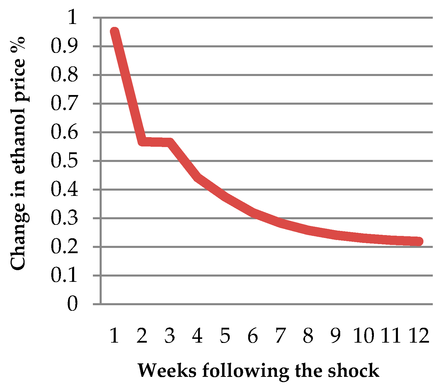
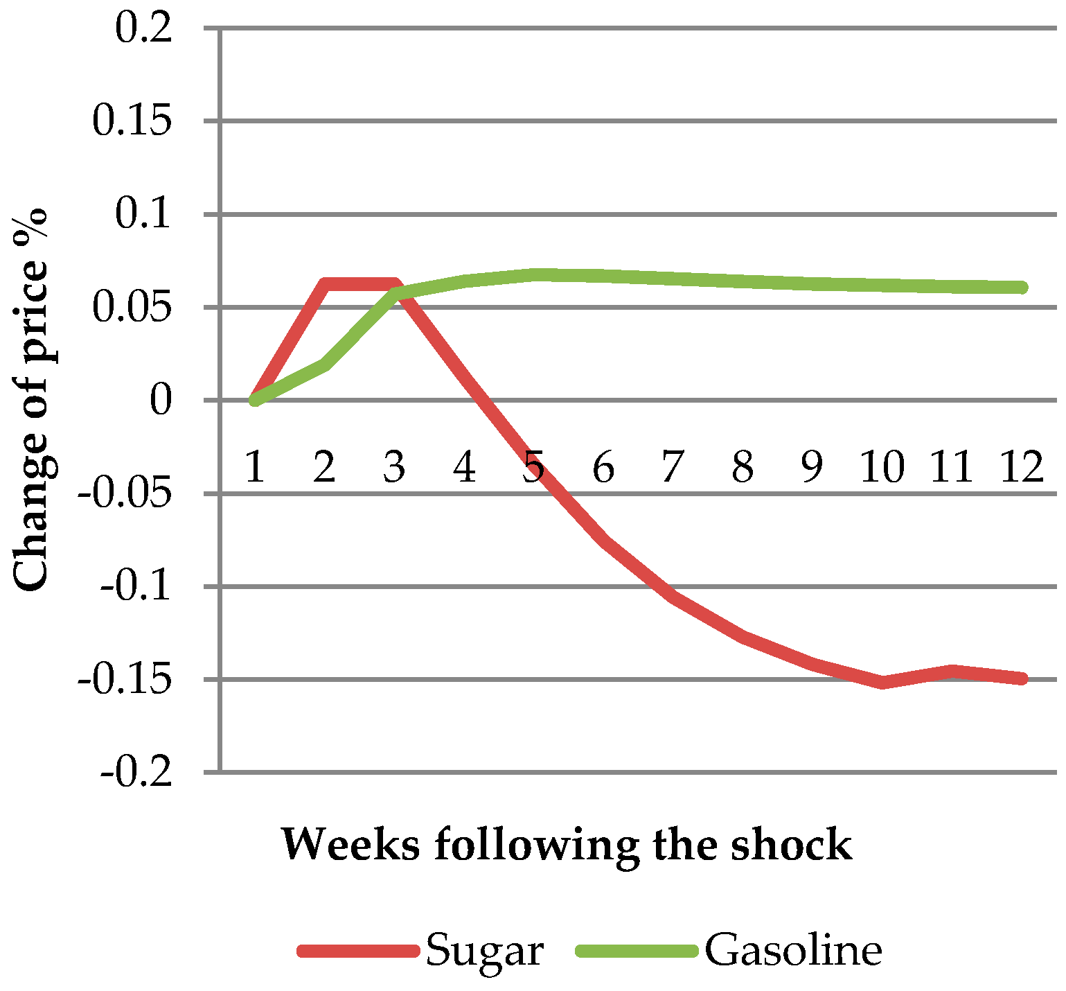
5.2.2. Impulse Response Analysis

In order to estimate the effect of each variable on the others, an impulse response analysis was carried out. Impulse response analysis allows us to quantify the effect of a unitary increase of one variable (the impulse) on other variables (response), including prospective values. In detail, the IRFs are used to track the responses of a system‘s variables to impulses of the system‘s shocks. IRFs measure the effect of a one standard-deviation shock of given variable on current and future values of variables. In particular, Figure 4 shows the accumulated IRFs of the ethanol price to a shock in sugar prices.

As shown in Figure 4 an increase in sugar prices causes a change in ethanol price of the same sign. In more detail, a shock of 1% in the sugar price induces an increase in the ethanol price from the first week. The magnitude of the response appeared to be an increase over time reaching a peak after 10 weeks (0.9%), and then it persists in subsequent periods. This is not surprising, given that the difference in the level of ethanol price is mainly associated with the quantity of sugarcane produced, as well as with the allocation of such material for sugar or ethanol production. Moreover, given the relevance of feedstock costs within the total costs of producing ethanol, it is not surprising to find that higher prices for sugar will lead to higher ethanol prices. On the contrary, an increase in the gasoline price is found to cause a decrease in ethanol prices (Figure 5).

Hence, if gasoline prices rise, its consumption decreases. This effect is reflected in the consumption of anhydrous ethanol which is used in blends with gasoline (27%). Consequently, the price of anhydrous ethanol drops, and this lower price is transmitted to pure ethanol because of the high correlation between the two markets [86].

At the same time, Figure 6 illustrates the accumulated IRFs of the sugar and gasoline price to a shock (1%) in the ethanol price. An increase in the ethanol price does not seem to produce an impact on both sugar and the gasoline prices.

5.2.3. Variance Decomposition Analysis

The empirical evidence from these results also found support in the VDC analysis carried out next. The VDC provided further evidence of relationships between the variables under investigation. The VDC showed the proportion of the forecast error of one variable due to the other variables. Therefore, VDC makes it possible to determine the relative importance of each variable in creating fluctuations in other variables [87]. As indicated in

Table 4. Variance decomposition analysis of ethanol after 12 periods (weeks).

Step	Ethanol	Sugar	Gasoline
1	20.980	0.788	78.233
2	22.700	6.777	70.523
3	23.639	7.872	68.489
4	23.146	9.474	67.380
5	22.905	10.211	66.884
6	22.755	10.613	66.632
7	22.687	10.798	66.515
8	22.657	10.882	66.462
9	22.644	10.918	66.438
10	22.638	10.934	66.428
11	22.636	10.940	66.424
12	22.635	10.943	66.422

, the variability of sugar prices explains 11% of the variance for ethanol prices, while gasoline prices account for 66% after 12 weeks.

At the same time, the variability of the price of sugar (

Table 5. Variance decomposition analysis of sugar after 12 periods (weeks).

Step	Ethanol	Sugar	Gasoline
1	0.000	100.000	0.000
2	0.035	78.783	21.182
3	0.032	79.193	20.775
4	0.049	78.536	21.415
5	0.065	78.417	21.518
6	0.077	78.340	21.583
7	0.083	78.310	21.606
8	0.087	78.297	21.616
9	0.088	78.291	21.620
10	0.089	78.289	21.622
11	0.089	78.288	21.623
12	0.089	78.288	21.623

) and of gasoline (

Table 6. Variance decomposition analysis of gasoline after 12 periods (weeks).

Step	Ethanol	Sugar	Gasoline
1	0.000	0.000	100.000
2	0.008	3.069	96.923
3	0.040	3.055	96.906
4	0.041	3.208	96.751
5	0.041	3.238	96.721
6	0.041	3.259	96.700
7	0.041	3.268	96.692
8	0.041	3.271	96.688
9	0.041	3.273	96.686
10	0.041	3.274	96.685
11	0.041	3.274	96.685
12	0.041	3.274	96.685

) after 12 weeks depends exclusively on the price of sugar and gasoline themselves (78% and 97%, respectively).

This analysis, on the one hand, supports the significant influence of both gasoline and sugar prices on ethanol prices; on the other hand, it confirms that rising ethanol prices are not directly causing inflated agricultural commodity prices [88].

6. Discussion and Conclusions

This study has aimed to examine price transmission patterns between Brazilian ethanol and related agricultural and energy markets. The links of this renewable market to fossil energy markets, on the one hand, and to agricultural raw product markets, on the other, were analysed using weekly prices of ethanol, sugar, and gasoline between November 2007 and November 2013. To investigate the relationships between these series, a co-integration analysis and a VECM were carried out. Moreover, IRFs and FEVD were computed in this model, in order to investigate the interrelationships within the sector.

Our results show that ethanol and gasoline, as well as ethanol and sugar price levels are linked in the long run by equilibrium parity. These links show that ethanol prices increment with an increase in both gasoline and sugar prices. The positive relationship between ethanol and sugar prices is not surprising, given the influence of feedstock costs within the total costs of producing ethanol (60%). Furthermore, gasoline prices may affect ethanol prices, because ethanol serves as a substitute for gasoline. The empirical results also show that sugar and gasoline prices drive ethanol prices in the short run.

Conversely, it was found that ethanol prices have limited power to influence food and energy prices. In fact, nowadays the variability of sugar prices depends especially on international sugar markets, while the Brazilian government establishes domestic gasoline prices. In particular, sugar prices will also increase as Brazil as the world’s major sugar producer and exporter influences the world sugar balance. Therefore, our analysis suggests that, for the markets and time span considered, ethanol prices are affected by both food and fuel prices, but there is no strong evidence that changes in biofuel prices affect food prices.

This study provide further evidence in favour of the “Food versus Fuel” debate. Concern over competition between biofuels and food production has been particularly acute, given the overwhelming use of food and feed crops for biodiesel production. To date, the literature has been very wide-ranging [32]. According to Hochman et al. [89] and Kristoufek et al. [90], the relationship between fuels and agri-food commodity prices depends on the market analysed (EU, US and Brazilian context), on the types of commodities, on the specification of the model and on the time series data and observation period (weekly, monthly or quarterly). Moreover, the dynamics of commodity prices are complicated and different factor may be affecting these markets [91]. The various calculations of the impacts of biofuel production on the mid-term projections of food and agricultural commodity prices are difficult to reconcile. This is largely due to the specific assumptions underlying each model, the scope of the studies (national/international), their time horizon, the choices of different policy scenarios, or even more simply the definition of “food prices” and of aggregate commodity prices [92]. For similar reasons, studies evaluating the impact of biofuel production on food and commodity prices to date do not provide a clear consensus.

According to different studies [46,48,90] we argue that this result does not imply that the introduction of ethanol has no impact on food prices. In fact, this study cannot capture the impact of biofuels on food prices, but only the linkages between fuel and food prices.

Some studies underline that the introduction of ethanol could have a lower impact on sugar prices. However, Brazil is a major food producer and exporter and official statistics demonstrate that the expansion of sugarcane planting has not affected the production of corn, soy, rice and beef, amongst other key commodities [93,94,95]. New land required for sugarcane production would be relatively small, and the same is true for the fall in other crops or livestock production [22]. Moreover, it is important to understand that almost half of all sugarcane harvested in Brazil is destined to sugar production, which is a food ingredient. It is also worth noting that sugarcane plantations are normally managed under a crop rotation system: sugarcane is a perennial plant that requires replanting after five to six years, at which point it is common to rotate the land to a grain crop like corn, soy or peanut.

Hence our analysis suggests that promoting ethanol in Brazil can be a useful tool to reduce both dependence on crude oil and GHG emissions [96,97,98]. Given his competitive advantage in ethanol production, the sugarcane industry is one of the pillars of the Brazilian economy. Brazilian ethanol is produced at low costs and its feasibility does not depend on subsidies. The competitive advantage from sugarcane ethanol, in terms of economic and environmental sustainability, also provides an opportunity to promote rural economies [17,18].

To conclude, our results contribute to the policy debate about biofuels as possible source of rises in agricultural commodity prices leading to food crises. We would like to underline that the policymakers could carefully distinguish between different biofuels. Differences in size and structure of the biofuels industry across the world, as well as differences in the feedstocks used by this sector, imply that policies should not be generalized [23]. According to Kristoufek et al. [90], the policymakers in any individual country have to be aware that biofuels are a broad phenomenon, with three leading players-the EU, the USA and Brazil. Significant development of advanced biofuels is necessary in order to promote biofuels that deliver substantial GHG savings (including LUC emissions) and reduce competition with food crops. In this contest, the European Commission developed Directive (EU) 2015/1513 with the aim of limiting the contribution of first generation biofuels towards attainment of the targets in the RED in favor of 2nd and 3rd generation biofuels.

Finally, the results of this study suggest that food-fuel linkage deserves much further investigation. The authors suggest that future study investigating the effect of the introduction of ethanol on food prices by using for example equilibrium model could support the results provide important information in order to complete the analysis.

References

1. Abbott, P.; De Battisti, B.A. Recent global food price shocks: Causes, consequences and lessons for African governments and donors. J. Afr. Econ. 2011, 20, i12–i62. [Google Scholar] [CrossRef]
2. Balcombe, K. The nature and determinants of volatility in agricultural prices: An empirical study from 1962–2008. FAO Commodity Market Rev. 2010, 1–24. [Google Scholar]
3. Sarris, A. Evolving structure of world agricultural trade and requirements for new world trade rule. In Proceedings of Food and Agriculture Organization of the United Nations-FAO Expert Meeting on “How to Feed the World in 2050” FAO, Rome, Italy, 24–26 June 2009; Available online: ftp://ftp.fao.org/docrep/fao/012/ak979e/ak979e00.pdf (accessed on 24 January 2014).
4. Gilbert, C.L. How to Understand High Food Prices. J. Agric. Econ. 2010, 61, 398–425. [Google Scholar] [CrossRef]
5. Gilbert, C.L.; Morgan, C.W. Food price volatility. Philos. Trans. R. Soc. Lond. B Biol. Sci. 2010, 365, 3023–3034. [Google Scholar] [CrossRef] [PubMed]
6. De Schutter, O. Food commodities speculation and food price crises: Regulation to reduce the risks of price volatility. United Nations Spec. Rapp. Right Food Brief. Note 2010, 2, 1–14. [Google Scholar]
7. Jacks, D.S.; O’Rourke, H.K.; Williamson, J.G. Commodity Price Volatility and World Market Integration since 1700. Rev. Econ. Statist. 2011, 93, 800–813. [Google Scholar] [CrossRef]
8. Huchet-Bourdon, M. Agricultural commodity Price volatility: An Overview. In OECD Food, Agriculture and Fisheries Working Papers; Organisation for Economic Co-operation and Development (OECD) Publishing: Paris, France, 2011; p. 52. [Google Scholar]
9. Muller, S.A.; Anderson, J.E.; Wallington, J.T. Impact of biofuels production and other supply and demand factors on food price increases in 2008. Biomass Bioenergy 2011, 35, 1623–1632. [Google Scholar] [CrossRef]
10. OECD-FAO. Agricultural Outlook 2011–2020. 2011. Available online: https://www.google.it/url?sa=t&rct=j&q=&esrc=s&source=web&cd=6&cad=rja&uact=8&ved=0ahUKEwjr_-nHgofMAhVCYQ8KHZewCTAQFghDMAU&url=https%3A%2F%2Fwww.donorplatform.org%2Findex.php%3Foption%3Dcom_cobalt%26task%3Dfiles.download%26tmpl%3Dcomponent%26id%3D1719%26fid%3D15%26fidx%3D0%26rid%3D1365%26return%3DaHR0cHM6Ly93d3cuZG9ub3JwbGF0Zm9ybS5vcmcvY29iYWx0L2NhdGVnb3J5LWl0ZW1zLzEtbGlicmFyeS84LWZvb2Qtc2VjdXJpdHk%252Fc3RhcnQ9MjA%253D&usg=AFQjCNExF9GlwBrP__b6WwkmDe82Hm1myQ (accessed on 3 February 2014).
11. Finco, A. Biofuels Economics and Policy-Agricultural and Environmental Sustainability; Franco Angeli: Milano, Italy, 2013; pp. 94–109. [Google Scholar]
12. Tyner, W.E. Biofuels and food prices: Separating wheat from chaff. Glob. Food Secur. 2013, 2, 126–130. [Google Scholar] [CrossRef]
13. Brons, M.; Nijkamp, P.; Pels, E.; Rietveld, P.A. A meta-analysis of the price elasticity of gasoline demand. A SUR approach. Energy Econ. 2008, 30, 2105–2122. [Google Scholar] [CrossRef]
14. Zhang, Z.; Lohr, L.; Escalante, C.; Wetzstein, M. Food versus fuel: What do price tell us? Energy Policy 2010, 38, 445–451. [Google Scholar] [CrossRef]
15. Ciaian, P.; Kancs, D. Interdependencies in the energy-bioenergy-food price systems: A cointegration analysis. Resour Energy Econ. 2011, 33, 326–348. [Google Scholar] [CrossRef]
16. Chinnici, G.; D’Amico, M.; Pecorino, B. Assessment and prospects of renewable energy in Italy. Calitatea 2015, 16, 126–134. [Google Scholar]
17. Chinnici, G.; D’Amico, M.; Rizzo, M.; Pecorino, B. Analysis of biomass availability for energy use in Sicily. Renew. Sustain. Energy Rev. 2015, 52, 1025–1030. [Google Scholar] [CrossRef]
18. Testa, R.; Foderà, M.; Di Trapani, A.M.; Tudisca, S.; Sgroi, F. Giant reed as energy crop for Southern Italy: An economic feasibility study. Renew. Sustain. Energy Rev. 2016, 58, 558–564. [Google Scholar] [CrossRef]
19. Kafle, K.; Pullabhotla, H.K. Food for the Stomach or Fuel for the Tank: What do Prices Tell Us? In Proceedings of the 2014 Annual Meeting, Minneapolis, MN, USA, 27–29 July 2014.
20. Havranek, T.; Irsova, Z.; Janda, K. Demand for gasoline is more price-inelastic than commonly thought. Energy Econ. 2012, 34, 201–207. [Google Scholar] [CrossRef]
21. Lora, E.E.S.; Palacio, J.C.E.; Rocha, M.H.; Reno, G.; Venturini, O.J.; del Olmo, O.A. Issues to Consider, Existing Tools and Constraints in Biofuels Sustainability Assessments. Energy 2011, 36, 2097–2110. [Google Scholar] [CrossRef]
22. De Souza Ferreira Filho, J.B.; Horridge, M. Ethanol expansion and indirect land use change in Brazil. Land Use Policy 2014, 36, 595–604. [Google Scholar] [CrossRef]
23. Popp, J.; Lakner, Z.; Harangi-Rákos, M.; Fári, M. The effect of bioenergy expansion: Food, energy, and environment. Renewable and Sustainable. Renew. Sustain. Energy Rev. 2014, 32, 559–578. [Google Scholar] [CrossRef]
24. Popp, J.; Harangi-Rákos, M.; Gabnai, Z.; Balogh, P.; Antal, G.; Bai, A. Biofuels and Their Co-Products as Livestock Feed: Global Economic and Environmental Implications. Molecules 2016, 21, 285. [Google Scholar] [CrossRef] [PubMed]
25. Ahlgren, S.; Di Lucia, L. Indirect land use changes of biofuel production—A review of modelling efforts and policy developments in the European Union. Biotechnol. Biofuels 2014, 7, 1. [Google Scholar] [CrossRef] [PubMed]
26. Searchinger, T.; Heimlich, R. Avoiding bioenergy competition for food crops and land. Creating a Sustainable Food Future. 2015, pp. 1–44. Available online: http://nocache.wri.org/sites/default/files/avoiding_bioenergy_competition_food_crops_land.pdf (accessed on 8 April 2015).
27. Searchinger, T.; Heimlich, R.; Houghton, R.; Dong, F.; Elobeid, A.; Fabiosa, J.; Tokgoz, S.; Hayes, D.; Yu, T. Use of US Croplands for Biofuels Increases Greenhouse Gases through Emissions from Land Use Change. Science 2008, 319, 1238–1240. [Google Scholar] [CrossRef] [PubMed]
28. Perimenis, A.; Walimwipi, H.; Zinoviev, S.; Muller-Langer, F.; Miertus, S. Development of a Decision Support Tool for the Assessment of Biofuels. Energy Policy 2011, 39, 1782–1793. [Google Scholar] [CrossRef]
29. Edwards, R.; Mulligan, D.; Marelli, L. Indirect land use change from increased biofuels demand. Comparison of models and results for marginal biofuels production from different feedstocks. Joint Research Centre (JRC) Scientific and Technical Reports: Ispra, Italy, 2010; Available online: http://www.eac-quality.net/fileadmin/eac_quality/user_documents/3_pdf/Indirect_land_use_change_from_increased_biofuels_demand_-_Comparison_of_models.pdf (accessed on 8 April 2015).
30. Delzeit, R.; Klepper, G.; Lange, K.M. Assessing the Land Use Change Consequences of European Biofuel Policies and its Uncertainties. Review of IFPRI study, study on behalf of the European Biodiesel Board by Kiel Institute for the World Economy: Kiel, Germany, 2011. Available online: http://www.ebb-eu.org/EBBpressreleases/Review_iLUC_IfW_final.pdf (accessed on 8 April 2015).
31. Zilberman, D.; Hochman, G.; Rajagopal, D. Indirect Land Use: One Consideration Too Many in Biofuel Regulation. Agric. Resour. Econ. Update 2010, 13, 1–4. [Google Scholar]
32. Bentivoglio, D.; Rasetti, M. Biofuel sustainability: Review of implications for land use and food price. REA 2015, 70, 7–31. [Google Scholar]
33. Finco, A.; Padella, M.; Bentivoglio, D.; Rasetti, M. Sostenibilità dei biocarburanti e sistemi di certificazione. EDA 2012, 2, 247–269. (In Italian) [Google Scholar]
34. Fatih, B. World energy outlook 2015. International Energy Agency, 2015; p. 1. Available online: http://www.worldenergyoutlook.org/weo2015/ (accessed on 20 January 2016).
35. International Energy Agency. Medium-Term Renewable Energy Market Report 2015. Available online: https://www.iea.org/Textbase/npsum/MTrenew2015sum.pdf (accessed on 20 January 2016).
36. Worldwatch Institute. Available online: http://www.worldwatch.org/biofuel-production-declines-0 (accessed on 12 March 2014).
37. REN21. Renewables 2015 Global Status Report. 2015. Available online: http://www.ren21.net/wp-content/uploads/2015/07/REN12-GSR2015_Onlinebook_low1.pdf (accessed on 3 February 2016).
38. De Freitas, L.C.; Kaneko, S. Is there a causal relation between ethanol innovation and the market characteristics of fuels in Brazil? Ecolog. Econ. 2012, 74, 161–168. [Google Scholar] [CrossRef]
39. UNICA-The Brazilian Sugarcane Industry Association. Available online: http://www.unicadata.com.br/historico-de-producao-e-moagem.php?idMn=32&tipoHistorico=4 (accessed on 29 April 2014).
40. UNICA. Detalhamento das exportações mensais de etanol pelo Brasil. 2014. Available online: http://www.unicadata.com.br/listagem.php?idMn=23 (accessed on 2 July 2014).
41. Crago, C.L.; Khanna, M.; Barton, J.; Giuliani, E.; Amaral, W. Competitiveness of Brazilian sugarcane ethanol compared to US corn ethanol. Energy Policy 2010, 38, 7404–7415. [Google Scholar] [CrossRef]
42. Shikida, P.F.A.; Finco, A.; Cardoso, B.F.; Galante, V.A.; Rahmeier, D.; Bentivoglio, D.; Rasetti, M. A comparison between ethanol and biodiesel production: The Brazilian and European experiences. In Liquid Biofuels: Emergence, Development and Prospects; Springer-Verlag: London, UK, 2014; pp. 25–53. [Google Scholar]
43. Martins-Filho, J.; Burnquist, H.L.; Vian, C.E.F. Bioenergy and the rise of sugarcane based ethanol in Brazil. Choices 2006, 21, 91–96. [Google Scholar]
44. Programa de Educação Continuada em Economia e Gestão de Empresas (PECEGE ESALQ/USP). Custos de produção de cana-de-açúcar, açúcar e etanol no Brasil: fechamento da safra 2012/2013; 1a Ediçao; Universidade de São Paulo, Escola Superior de Agricultura “Luiz de Queiroz”/Departamento de Economia, Administração e Sociologia: Piracicaba, SP, Brazil, 2013; pp. 23–44. (In Portuguese) [Google Scholar]
45. Hochman, G.; Sexton, S.; Zilberman, D. Food and Biofuel in Global Environment. In Handbook of Bioenergy Economics and Policy; Khanna, M., Scheffran, J., Zilberman, D., Eds.; Springer Science & Business Media: New York, NY, USA, 2009; pp. 267–286. [Google Scholar]
46. Kristoufek, L.; Janda, K.; Zilberman, D. Mutual Responsiveness of Biofuels, Fuels and Food Prices. CAMA Working Paper 38. 2012. Available online: http://cama.crawford.anu.edu.au/pdf/working-papers/2012/382012.pdf (accessed on 24 July 2014).
47. Vacha, L.; Janda, K.; Kristoufek, L.; Zilberman, D. Time-Frequency Dynamics of Biofuels Fuels-Food System. Energ. Econ. 2013, 40, 233–241. [Google Scholar] [CrossRef]
48. Zilberman, D.; Hochman, G.; Rajagopal, D.; Sexton, S.; Timilsina, G. The impact of biofuels on commodity food prices: Assessment of Findings. Am. J. Agr. Econ. 2013, 95, 275–281. [Google Scholar] [CrossRef]
49. Serra, T.; Zilberman, D. Biofuels-related price transmission literature: A review. Energ. Econ. 2013, 37, 141–151. [Google Scholar] [CrossRef]
50. Zhang, Z.; Lohr, L.; Escalante, C.; Wetzstein, M. Ethanol, corn, and soybean price relations in a volatile vehicle-fuels market. Energies 2009, 2, 230–339. [Google Scholar] [CrossRef]
51. Saghaian, S.H. The impact of the oil sector on commodity prices: Correlation or causation? J. Agric. Appl. Econ. 2010, 42, 477–485. [Google Scholar] [CrossRef]
52. Serra, T.; Zilberman, D.; Gil, J.M.; Goodwin, B.K. Nonlinearities in the US corn-ethanol-oil-gasoline price system. Agric. Econ. 2011, 42, 35–45. [Google Scholar] [CrossRef]
53. Du, X.; McPhail, L. Inside the black box: The rice linkage and transmission between energy and agricultural markets. Energy J. 2012, 33, 171–194. [Google Scholar] [CrossRef]
54. Qiu, C.; Colson, G.; Escalante, C.; Wetzstein, M. Considering macroeconomic indicators in the food before fuel nexus. Energy Econ. 2012, 34, 2021–2028. [Google Scholar] [CrossRef]
55. Wixson, S.E.; Katchova, A.E. Price asymmetric relationships in commodity and energy markets. In Proceedings of the 123rd European Association of Agricultural Economists (EAAE) Seminar, Dublin, Ireland, 23–24 February 2012.
56. Gardebroek, C.; Hernandez, M.A. Do energy prices stimulate food price volatility? Examining volatility transmission between US oil, ethanol and corn markets. Energy Econ. 2013, 40, 119–129. [Google Scholar] [CrossRef]
57. Busse, S.; Brümmer, B.; Ihle, R. Interdependencies between fossil fuel and renewable energy markets: The German biodiesel market. Diskussionspapiere//Department für Agrarökonomie und Rurale Entwicklung, 2010. Available online: http://www.econstor.eu/handle/10419/45604 (accessed on 24 July 2014).
58. Busse, S.; Brümmer, B.; Ihle, R. Price formation in the German biodiesel supply chain: A Markov-switching vector error correction modeling approach. Agric. Econ. 2012, 43, 545–560. [Google Scholar] [CrossRef]
59. Peri, M.; Baldi, L. Vegetable oil market and biofuel policy: an asymmetric cointegration approach. Energy Econ. 2010, 32, 687–693. [Google Scholar] [CrossRef]
60. Hassouneh, I.; Serra, T.; Goodwin, B.K.; Gil, J.M. Non-parametric and parametric modeling of biodiesel, sunflower oil, and crude oil price relationships. Energy Econ. 2012, 34, 1507–1513. [Google Scholar] [CrossRef]
61. Rajcaniova, M.; Pokrivcak, J. The impact of biofuel policies on food prices in the European Union. Ekon. Cas. /J. Econ. 2011, 5, 459–471. [Google Scholar]
62. Bentivoglio, D.; Finco, A.; Bacchi, M.R.P.; Spedicato, G. European biodiesel market and rapeseed oil: What impact on agricultural food prices? Int. J. Global Energy Issues 2014, 37, 220–235. [Google Scholar] [CrossRef]
63. Rapsomanikis, G.; Hallam, D. Threshold cointegration in the sugar-ethanol-oil price system in Brazil: evidence from nonlinear vector error correction models. FAO commodity and trade policy research working paper 22. 2006. Available online: http://sharing.mywordsolution.com/xtringfiles/240_thresholdVectorErrorCorrection.pdf (accessed on 24 July 2014).
64. Balcombe, K.; Rapsomanikis, G. Bayesian estimation of nonlinear vector error correction models: the case of sugar-ethanol-oil nexus in Brazil. Am. J. Agric. Econ. 2008, 90, 658–668. [Google Scholar] [CrossRef]
65. Serra, T.; Zilberman, D.; Gil, J. Price volatility in ethanol markets. Eur. Rev. Agric. Econ. 2011, 38, 259–280. [Google Scholar] [CrossRef]
66. Serra, T. Volatility spillover between food and energy market: A semiparametric approach. Energy Econ. 2010, 33, 1155–1164. [Google Scholar] [CrossRef]
67. Wright, W. The economics of grain price volatility. Appl. Econ. Perspect Policy 2011, 33, 32–58. [Google Scholar] [CrossRef]
68. Engle, R.; Granger, C. Cointegration and error correction representation, estimation and testing. Econometrica 1987, 55, 251–276. [Google Scholar] [CrossRef]
69. Granger, C.W.J. Some Recent Developments in a Concept of Causality. J. Econometrics 1988, 39, 199–211. [Google Scholar] [CrossRef]
70. Myers, R.J. Time series econometrics and commodity price analysis: A review. Rev. Mark. Agric. Econ. 1992, 62, 167–181. [Google Scholar]
71. Erjavec, N.; Cota, B. Macroeconomic granger-causal dynamics in Croatia: evidence based on a vector error-correction modelling analysis. Ekonomski pregled 2003, 54, 139–156. [Google Scholar]
72. Pfaff, B. Analysis of Integrated and Cointegrated Time Series with R, 2nd ed.; Springer: New York, NY, USA, 2008. [Google Scholar]
73. Pfaff, B. Var, svar and svec models: Implementation within R package vars. J. Stat. Softw. 2008, 27, 1–32. Available online: http://vps.fmvz.usp.br/CRAN/web/packages/vars/vignettes/vars.pdf (accessed on 22 July 2014). [Google Scholar] [CrossRef]
74. Zafeiriou, E.; Arabatzis, G.; Tampakis, S.; Soutsas, K. The impact of energy prices on the volatility of ethanol prices and the role of gasoline emissions. Renew. Sust. Energ. Rev. 2014, 33, 87–95. [Google Scholar] [CrossRef]
75. Haixia, W.; Shiping, L. Volatility spillovers in China’s crude oil, corn and fuel ethanol markets. Energy Policy 2013, 62, 878–886. [Google Scholar] [CrossRef]
76. Granger, C.W. Some recent development in a concept of causality. J. Econ. 1988, 39, 199–211. [Google Scholar] [CrossRef]
77. Miller, S.M.; Russek, F.S. Co-integration and error-correction models: The temporal causality between government taxes and spending. Southern Econ. J. 1990, 57, 221–229. [Google Scholar] [CrossRef]
78. Center for Advanced Studies on Applied Economics (CEPEA). Center for Advanced Studies on Applied Economics (CEPEA), Alcohol and sugar prices datasets. Available online: http://cepea.esalq.usp.br/alcool/ (accessed on 29 April 2014).
79. Agência Nacional do Petróleo, Gás Natural e Biocombustíveis-ANP. Available online: http://www.anp.gov.br/preco/ (accessed on 29 April 2014).
80. Dickey, D.A.; Fuller, W.A. Distribution of the Estimators for Autoregressive Time Series with a Unit Root. J. Amer. Statistical Assoc. 1979, 74, 427–431. [Google Scholar]
81. Johansen, S. Statistical analysis of cointegration vectors. J. Econ. Dynam. Control 1988, 12, 231–254. [Google Scholar] [CrossRef]
82. Tenkorang, F.; Dority, B.L.; Bridges, D.; Lam, E. Relationship between ethanol and gasoline: AIDS approach. Energy Econ. 2015, 50, 63–69. [Google Scholar] [CrossRef]
83. Barros, S. Brazil-Biofuels-Ethanol and biodiesel. GAINT Report Number: BR15006; 2015. Available online: http://gain.fas.usda.gov/Recent%20GAIN%20Publications/Biofuels%20Annual_Sao%20Paulo%20ATO_Brazil_8-4-2015.pdf (accessed on 3 February 2016). [Google Scholar]
84. Granger, C.W.J. Testing for Causality: A personal viewpoint. J. Econ. Dynam. Control 1980, 2, 329–352. [Google Scholar] [CrossRef]
85. Pala, A. Structural Breaks, Cointegration, and Causality by VECM Analysis of Crude Oil and Food Price. Int. J. Energy Econ. Policy 2013, 3, 238–246. [Google Scholar]
86. Marjotta-Maistro, M.C. Desafios e perspectivas para o setor sucroenergético do Brasil. 2011. Available online: http://hdl.handle.net/123456789/589 (accessed on 22 May 2014).
87. Ratanapakorn, O.; Sharma, S.C. Dynamic analysis between the US stock returns and the macroeconomic variables. Appl. Finan. Econ. 2007, 17, 369–377. [Google Scholar] [CrossRef]
88. Chagas, A.L.S. Etanol ou Alimento: Existe Esse Trade-off? Informaçoes FIPE: Sao Paulo, Brazil, 1 March 2010; pp. 11–16. (In Portuguese) [Google Scholar]
89. Hochman, G.; Rajagopal, D.; Timilsina, G.; Zilberman, D. Quantifying the causes of the global food commodity price crisis. Biomass Bioenerg. 2014, 68, 106–114. [Google Scholar] [CrossRef]
90. Kristoufek, L.; Janda, K.; Zilberman, D. Price transmission between biofuels, fuels, and food commodities. Biofuels, Bioprod. Biorefin 2014, 8, 362–373. [Google Scholar] [CrossRef]
91. Nazlioglua, S.; Erdemb, C.; Soytasc, U. Volatility spillover between oil and agricultural commodity markets. Energy Econ. 2012, 36, 658–665. [Google Scholar] [CrossRef]
92. Gerber, N.; van Eckert, M.; Breuer, T. Biofuels and food prices: A review of recent and projected impacts. RIO9-World Climate & Energy Event 2009, 17, 19. [Google Scholar]
93. Goldemberg, J.; Coelho, S.T.; Guardabassi, P. The sustainability of ethanol production from sugarcane. Energy policy 2008, 36, 2086–2097. [Google Scholar] [CrossRef]
94. Féres, J.; Reis, E.; Speranza, J. Assessing the “food-fuel-forest” competition in Brazil: Impacts of sugarcane expansion on deforestation and food supply. 2010. Available online: http://cerdi.org/uploads/sfCmsContent/html/323/Feres_foodfuelforest.pdf (accessed on 18 November 2015).
95. Sousa, E.L.L.; Macedo, I.C. Ethanol and bioelectricity-Sugarcane in the future of the energy matrix; União da Indústria de Cana-de-Açúcar (UNICA): São Paulo, SP, Brazil, 2010; pp. 1–315. [Google Scholar]
96. Finco, A.; Bentivoglio, D.; Nijkamp, P. Integrated evaluation of biofuel production options in agriculture: An exploration of sustainable policy scenarios. IJFIP 2012, 8, 173–188. [Google Scholar] [CrossRef]
97. Rasetti, M.; Finco, A.; Bentivoglio, D. GHG balance of biodiesel production and consumption in EU. Int. J. Global Energy Issues 2014, 37, 191–204. [Google Scholar] [CrossRef]
98. Padella, M.; Finco, A.; Tyner, W.E. Impacts of biofuels policies in the EU. Econ. Energy Environ. Policy 2012, 1, 87–104. [Google Scholar] [CrossRef]
Figure 1. World Ethanol and Biodiesel production 1975–2012 [36].
Energies 09 00464 g001
Figure 2. Ethanol production in Brazil from 1980 to 2013 [39].
Energies 09 00464 g002
Figure 3. Indexed price series %.
Energies 09 00464 g003
Figure 4. Ethanol response to a shock to the sugar prices.
Energies 09 00464 g004
Figure 5. Ethanol response to a shock to the gasoline prices.
Energies 09 00464 g005
Figure 6. Sugar and gasoline responses to a shock to ethanol prices.
Energies 09 00464 g006