Review

Variability Characteristics of European Wind and Solar Power Resources—A Review

Department of Electric Power Engineering, Norwegian University of Science and Technology, Trondheim N-7034, Norway
*
Author to whom correspondence should be addressed.
Energies 2016, 9(6), 449; https://doi.org/10.3390/en9060449
Submission received: 18 December 2015 / Revised: 27 May 2016 / Accepted: 31 May 2016 / Published: 20 June 2016

Abstract

:
This paper reviews the most recent and relevant research into the variability characteristics of wind and solar power resources in Europe. The background for this study is that wind and solar resources will probably constitute major components of the future European power system. Such resources are variable, and EU plans to balance the variability with more grids and demand response. Thus, planning for the future power system requires an in-depth understanding of the variability. Resource variability is a multi-faceted concept best described using a range of distinct characteristics, and this review is structured on the basis of seven of these: Distribution Long-Term (hours to years), Distribution Short-Term (less than one hour), Step Changes, Autocorrelation, Spatial Correlation, Cross Correlation and Predictable Patterns. The review presents simulations and empirical results related to resource variability for each of these characteristics. Results to date reveal that the variability characteristics of the future power system is limited understood. This study recommends the development of a scheme for greater systematic assessment of variability. Such a scheme will contribute to the understanding of the impacts of variability and will make it possible to compare alternative power production portfolios and impacts of grid expansions, demand response and storage technologies.

1. Introduction

1.1. Background

The need to reduce greenhouse gas (GHG) emissions is widely accepted, and a transformation of the energy system will represent an important contribution towards these reductions. The European Union (EU) has specified a target of a 40% cut in GHG emissions compared to 1990 levels and has agreed that renewable energy sources (RES) should constitute a minimum 27% share of energy consumption by 2030. Furthermore, the EU has stipulated a long-term goal to reduce GHG emissions by 80%–95% compared to 1990 levels by 2050 [1]. The Energy Roadmap 2050 explores the different ways in which a transition of the energy system might take place in order to achieve the GHG reduction target. Low emission scenarios in the Roadmap show that electricity will constitute a much larger share of the energy system than at present. The relative share of the electricity in the energy system may be almost doubled in 2050 compared to 2011. The share of RES in electricity consumption must rise substantially in all scenarios, achieving 64% in a High Energy Efficiency scenario and 97% in a High Renewables scenario. In the High Renewables scenario, wind power provides more electricity than any other technology. The Roadmap also indicates that solar power will be an important resource in the future low-carbon power system. The expansion of variable renewable electricity is already progressing rapidly, with worldwide annual growth rates for wind and solar PV of 21% and 55%, respectively, from end-2008 to 2013. In 2013, Denmark, Germany and Spain had renewable electricity generation shares of 56%, 25% and 42% respectively, with more than half of this share being from wind and solar energy in each country [2].
The European Council of October 2014 called for all EU Member States to achieve interconnections of at least 10% of their installed electricity production capacity by 2020. This means that each Member State should have in place cables that allow at least 10% of nationally produced electricity to be exported to its neighbouring countries. One of the reasons for the requirement is that electricity grids better can manage increasing level of renewables, particularly variable renewables like wind and solar. The EU is looking into raising the target to 15% by 2030. However, higher targets may be case specific depending among other on the geographical position of a country and its energy mix, for example the weight of renewables in it [3]. The EU Commission also consider demand side flexibility as an important contribution to smooth out future variable production from RES [4].
In Northern Europe in general and for Germany in particular the hydropower system in Scandinavia is considered as an opportunity for balancing variable renewable production. This is among other described by the Germany Advisory Council on Environment in their study “Pathways to 100% renewable electricity system” [5]. Norway and Sweden have approximately 116 TWh in hydro storage installations, and the hydropower reservoirs in Norway constitutes about half of the total reservoir capacity in Europe [6]. In periods with surplus in the production in Germany (or Northern Europe), the hydropower production in Scandinavia can be quickly regulated down and the consumption partly supplied by imports from Continental Europe. In periods with deficits in wind and solar power production in Germany and neighbouring countries, the hydro power production in Scandinavia can easily be increased to meet the demand in the deficit areas.

1.2. The Scope of this Paper

As mentioned above, a major challenge linked to RES is the variability of the most promising resources. Weather conditions determine the output from variable renewable resources, i.e., the production cannot be adjusted in the same way as of dis-patchable power plants. Variable RES generation does not perfectly follow the load, so integration costs occur when accommodating variables RES in a power system [7]. Variable generation sources include solar, wind, ocean and some run-of-river hydro technologies.
Variability cannot be expressed using a single measurable parameter. It is a multi-faceted concept best described by a range of distinct properties [8]. Thus, variability has different characteristics and these characteristics may vary according to the time scale over which they are measured. It is important to understand these variability characteristics in order to optimally design and operate the future power system.
The difference between the power load and the variable RES production is often called the net load. Since the production and the load in a power system have to always be balanced, the net load has to be supplied by dis-patchable production or from some kind of storage. Power production from wind and solar resources have very low marginal costs, and increasing shares of wind and solar production results in periods with low and even negative prices. This will result in reduced profitability for conventional dis-patchable technologies like gas turbines, coal and nuclear plants. In the longer run high fixed cost technologies may leave the market and there will be less capacity left for balancing the net load [9]. The literature describes different options for balancing power production from variable RES, mainly large scale energy storage, expansion of interconnection capacity, demand response, flexible power plants, market integration and system operation closer to real time [10,11]. In order to be able to evaluate a cost-efficient combination of these options, the aim of this paper is to establish a state-of-the-art overview of the knowledge about the variability characteristics of renewable resources for the European region in a long term perspective.
Many papers have been published on the variability of RES production in relation to net load. It is likely that the load profile will change in the future, on the one hand due to reduced energy consumption resulting from e.g., zero-energy homes and, on the other, the charging of electric vehicles (EVs), etc. that will increase consumption. Studies of future net load should be based on the anticipated future load profile or scenarios for different possible future load profiles. In this review, we primarily focus on resource variability in order to limit the scope of the paper. Knowledge about the future load profile should be a topic for a separate review.
There are also papers about costs for integration of renewables, e.g., [7,12,13] has shorter time-perspective than our study and quantify costs by use of present power market prices and conventional thermal production. However, according to [12] “…there are a number of integration options that can effectively reduce integration costs… Most integration options are costly and it is unclear to which extend these options are economically efficient. Deriving an efficient mix of integration options requires carefully analysis of power system considering the complex integration of variable renewables, other generation technologies and integration options...”. The paper mentions cross-border transmission, demand flexibility and different types of storage as important integration options. It also mentions the impact of geographical correlation of variable RES for connections of regions. We do not focus on costs in this study, but aim instead to contribute to increased understanding of the variability characteristics of wind and solar resources in Europe in a long term perspective. Based on the knowledge of the variable characteristics, the contribution of and costs for alternative integration options can be studied in a next step beyond this paper. By review of available scientific literature, we aim to find out what is the knowledge of the variability of future wind and solar power production in Europe along two dimensions:
  • How localisation, share and mix of wind and solar power production can contribute to smooth the output (impact of geographical correlation). The aggregated power production from several variable resources may be smoother than the output from each of the resources. e.g., according to [14], the challenges of integrating variable generation into power systems to a large extent depend on the penetration level, the mix of wind and solar and the regional circumstances. Given EU’s ambition for increases of wind and solar power production and for increased integration of the power system, we review in this paper what is the knowledge of how different penetration levels of wind and solar power production, the mixes of the resources and the localisation of the resources can smooth out variability.
  • How the aggregated wind and solar power production will vary in different time perspectives in order to be able to study how the variability can be balanced by measures with different properties. According to among other [11], there are large uncertainties related to how much demand response which will be available in a future power system. There is probably more flexibility available in the short time perspective than in a longer perspective. The paper studies the impacts of five options for integration of variable RES at minimum cost in Western-Europe in 2050 and assumes certain quantities of flexibility in demand. Instead of assuming specific quantities of demand, it is possible to turn the perspective the other way around. Based on knowledge of variability from wind and solar power production it is possible to study the impacts on the power system dis-patch and costs if demand flexibility contributes with different level of responses in different time perspectives. Furthermore, different types of storage have different properties. Thus, it is important to understand how an aggregated wind and solar power production in Europe varies in different time perspectives to be able to assess which type of storage can balance which part of the variability. E.g., according to [15] there are presently three alternatives for long term storage in the power system: pumped-storage-hydro power or hydropower reservoirs, compressed-air-energy-storage (CAES) and chemical hydrogen storage. Furthermore, as mentioned above conventional dis-patchable technologies with high fixed costs may leave the market in the long run. Both CAES and hydrogen have high up-front costs and also other disadvantages [15] in its present form while the hydropower system in Scandinavia can already to some degree be used for balancing variable production if the interconnectors are increased [6]. Thus, it is of particular interest to understand how often long lasting periods with low production from wind and solar resources will occur.
Our focus on the variability of wind and solar production is also motivated by the IEA ECES26 report (International Energy Agency, Electric Energy Storage) [16]. This report includes a survey of 16 relevant studies with respect to assessment of storage demand for Germany and Europe. It concludes that robust results about future need for specific technologies cannot be derived from the studies, due to their different assumptions about the future. As an alternative, assessing the overall need for balancing is promising. Therefore, sound derivations of need for balancing measures require, locally based assessment while estimates of the need of specific storage options according to the report seem to be almost meaningless. The “need for balancing” in [16] is the variable production from wind and solar resources minus the load, i.e., the net load. Except that we have chosen not to include load at this stage, our approach is in accordance with the recommendations from the IEA expert group. The review in this article focuses on Europe because of the specific EU-stipulated RES contribution targets and also because of EUs ambitions and plans for solution of the variability challenge. Given the EU target of increased integration of the power system, the review employs a wide range perspective. In case of characteristics for which only limited results are available, single sites results are considered. Results from other regions are included when only limited EU results are available.
According to the EU Energy Roadmap 2050, wind and solar resources will make considerably greater contributions to the future power system than other renewable resources, including tidal power. For example, in the High RES scenario, wind power will constitute 44% of installed power capacity in 2050, solar 27%, and other variable renewables only 1.4%. Based on the EU Road Map scenarios, we will limit our study to the variability of wind and solar resources.
In summary, the overall storyline for this review is an integrated European power system in a long term perspective (2050), with very high shares of variable wind and solar power production and which aims to use interconnectors, demand response and storage as much as possible to balance the variability. What is the knowledge of the variability in such a power system?

1.3. Methodology/Structure of Report

We started the review with identification of variable characteristics. The identification was based on findings in the scientific literature. The characteristics are described in Section 2. In this Section, the choice of structure is compared with the few other structures of RES variability characteristics we found in scientific papers. In the next step, scientific papers were studied in order to identify the knowledge front for each characteristic in Europe. We studied the knowledge front for both onshore and offshore wind, for solar resources and for wind and solar resources in combination. Even though we focused on the variability of the natural resources, we included papers about e.g., net load if those papers provided relevant results for our scope. We focused on scientific papers from the most recent years. However, if few results were published the recent years, we also tried to include older results. Section 3 describes the findings for Europe for each of the characteristics. Section 3.1 describes analytical studies that are referred to repeatedly in this paper. Section 3.9 provides a structured summary of the variability characteristics and their respective research fronts. In Section 4 we describe how the variability characteristics relate to the power system. Section 5 discusses the findings and identifies the research gap.

2. Variability Characteristics

In this section, different variability characteristics are identified based on the articles reviewed. A large number of scientific articles have been published addressing the variability of renewable resources. However, we found a limited literature that presents a structured overview of various variability characteristics and their respective research fronts. We chose to structure the review according to the following variability characteristics: Distribution Long Term, Distribution Short Term, Step Changes, Autocorrelation, Spatial-correlation, Cross-correlation and Predictable Pattern.
Some variability characteristics are identified based on a paper analyzing solar, wind and tidal resources by focusing on a small geographical region in the UK [
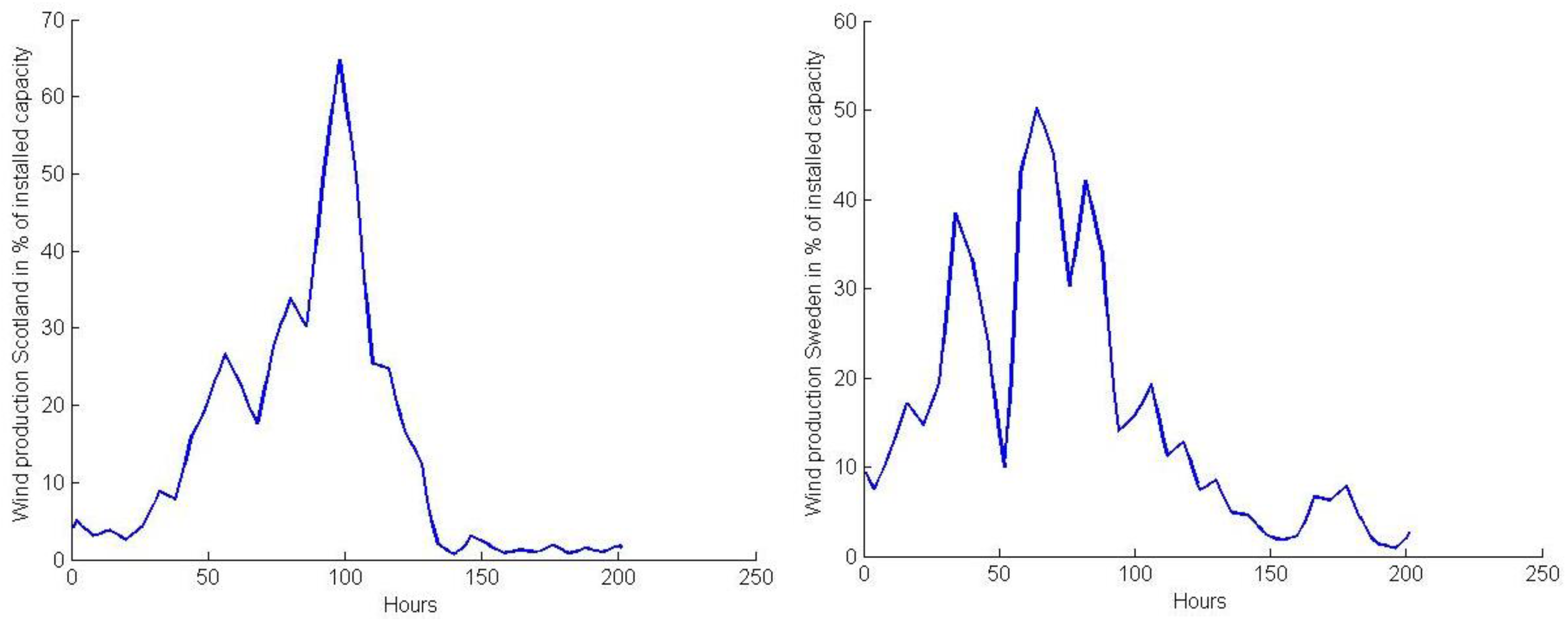
8]. Distribution is one of several variability characteristics. It can be defined as discrete power outputs recorded during stipulated time periods, and assessed over a longer period of time. For the purposes of this review, we have chosen to split “Distribution” into two categories; Short-Term (minutes, less than one hour) and Long-Term (one hour or more). There are several reasons for this subdivision:
  • Several power markets operate with an hourly resolution (Day-ahead Market).
  • Often, a variety of technologies will be used for balancing short-term (e.g., batteries) and longer-term variations (e.g., thermal plants with start-up costs).
  • Databases (at least in the case of wind resources) often have a resolution of one or several hours (e.g., see examples in [17]).
Several of the papers reviewed refer to ‘Step Changes’ as a variability characteristic. Step changes are changes in resource availability that occur over short time steps ranging from minutes to a few hours, and is the third characteristic that we review in this study. Another variable characteristic is Autocorrelation [
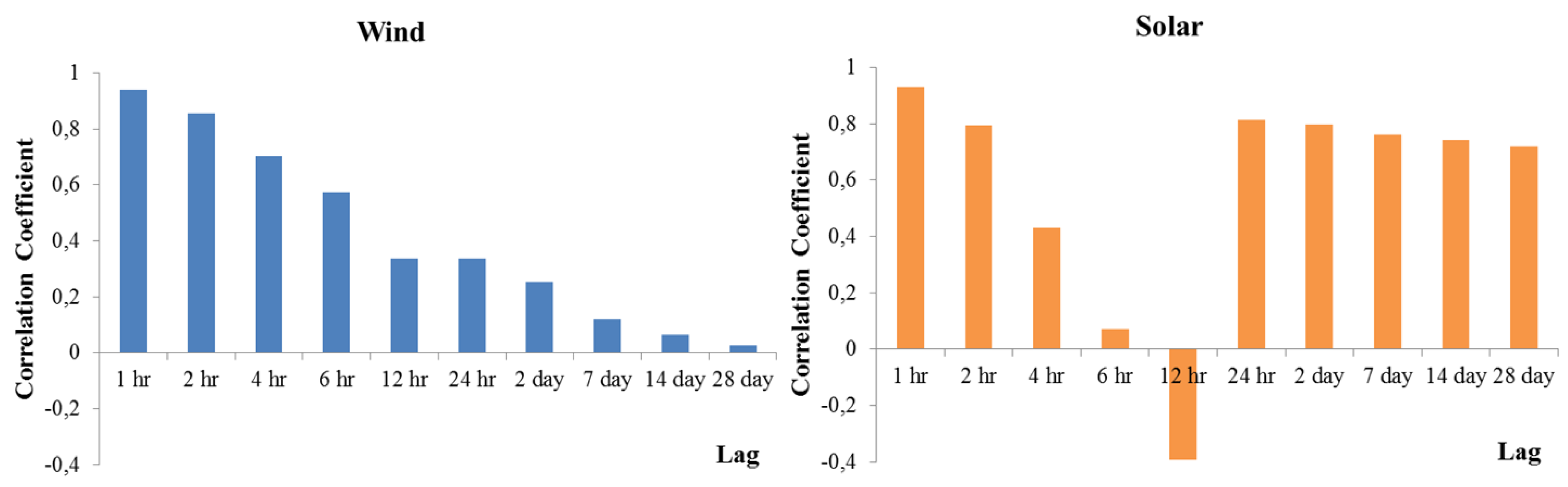
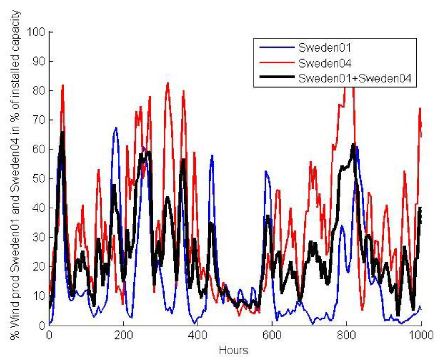
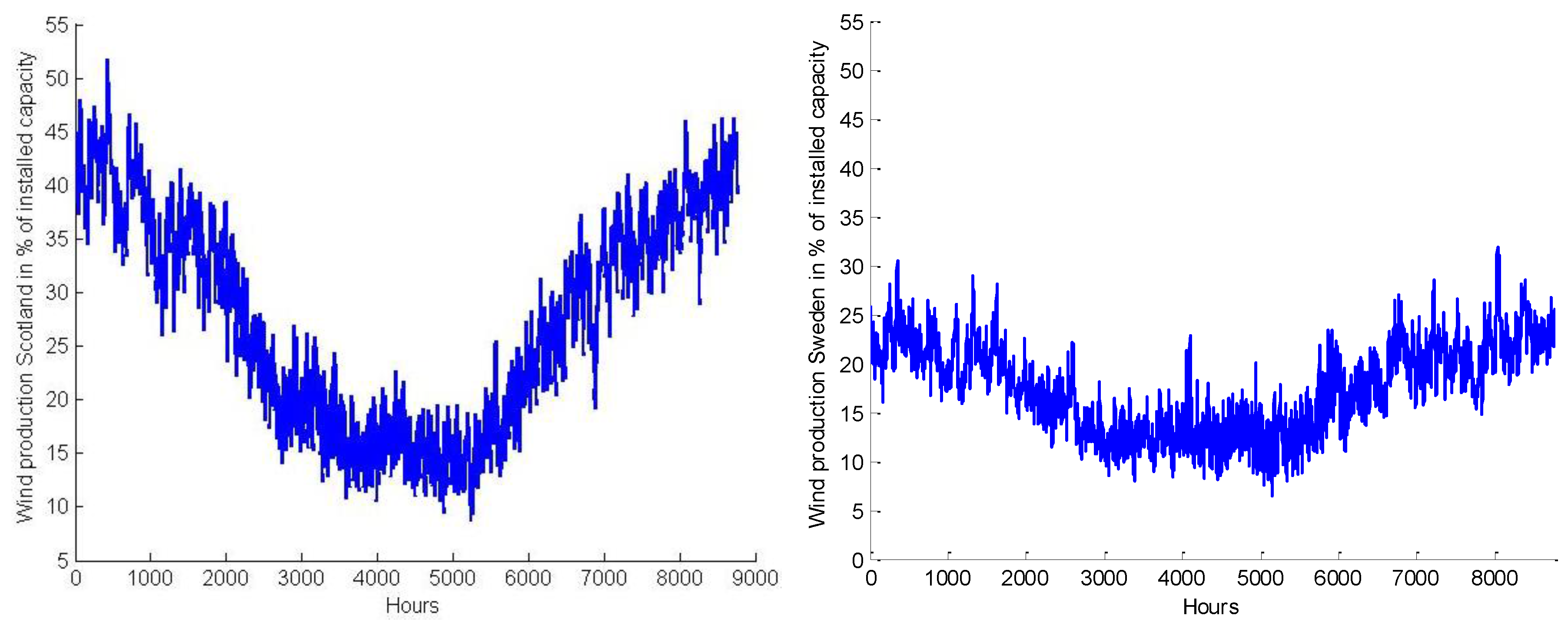
8]. Autocorrelation can be defined as the “existence of statistical dependence among successive values of the same variable”, and this is the fourth characteristic we discuss. The correlation of wind speed records between spatially distributed sites, and the corresponding correlation of solar radiation records for distributed sites have been, and still are, the focus of many research projects. For this reason, we identify Spatial Correlation as one of the variability characteristics. Wind and solar resources may exhibit different diurnal and seasonal patterns. However, they also complement each other to some degree. In studies of future power systems in which renewables make major contributions, it is useful to study the characteristic called Cross Correlation. Wind, solar and tidal resources also exhibit predictable patterns [8]. We have chosen to identify the annual and diurnal Predictable Patterns of renewables as a distinctive variability characteristic. Pattern prediction for wind and solar resources is a complex process, and forecasting is a topic addressed in many scientific papers. Unpredictability could also have been considered as a variability characteristic, but is not included in this review in order to limit scope of the study.
A recent study about variability of wind and solar power production in the present European power system includes the several of the same characteristics as discussed in this paper [18]. The paper do not used the same names of the characteristics as in this paper, but the content is mainly the same. The paper has some additional characteristics related to the demand, e.g., surplus in net load. Surplus in net load is an important aspect of a system with high shares of variable renewable production. It should be added in further extensions of this work with future load profiles included.
There are studies which categorize variability properties of RES related to the power system costs the property causes, e.g., [14]. In this study variable production is split in uncertain, location-specific and temporal variability. Uncertain includes the limited predictability of inherent natural variations of wind speed or solar irradiation. This property is the same as our Unpredictability characteristic. Location-specific is costs which occur because the primary energy carrier of wind and power cannot be transported like fossil or nuclear fuels. The location specific property is related to our Spatial Correlation characteristic. However, the perspectives are very different: e.g., [14] discusses the location specific costs while our study discusses how spatial (non) correlation can be used to smooth out variability (in the Conclusion section). Finally, according to [14] temporal variability has two impacts. The first one is increased ramping and cycling, and the second one is temporal matching of variable RES supply profiles with demand. Ramping and cycling is correspondent to our characteristic Step Changes. Again, the perspectives of our study and [14] is very different: [14] seems to have focus more on the present system than our study and assumes that demand is fairly price-inelastic while our study focuses on establish knowledge to be able to assess which parts of the variability can be balanced by demand flexibility.
Each of the characteristics is discussed in detail in the following sections. For each of the seven characteristics we provide a general description and a description of the knowledge front for onshore and offshore wind and solar power production for Europe.

3. Knowledge Front for Wind and Solar Variability per Characteristic

3.1. Relevant Simulation Studies

The following provides a description of simulation studies that will be referred to several times in the subsequent discussions.

3.1.1. A Simulation of Large-Scale Wind Power Production Based on Reanalysis Data

This is unpublished work that we include in this review to illustrate some of the variability characteristics. A method developed as part of the EU-funded project TradeWind was used to calculate wind data series [19,20]. Hourly time series for wind speed and power production have been developed covering a 64-year period from 1950 to 2013. The wind speed time series are based on NCEP (U.S. National Centre for Environmental Prediction) Reanalysis data taken from the website of the NOAA/OAR/ESRL PSD in Boulder, Colorado, USA [21]. The reanalysis dataset has a temporal resolution of 6 h and a spatial resolution of 2.5 degrees in both latitude and longitude. A two-dimensional linear interpolation of neighbouring reanalysis points is applied to obtain wind speeds at the selected locations (nodes). A linear interpolation of the 6-hourly values is used to generate hourly values. Wind speeds are adjusted using country-specific factors. Since wind speed values are averaged and smoothed out, and because the wind energy output data represents that from many wind turbines, a regional power curve is used for the computation [19]. Several of the illustrations in this paper are based on the geographical locations set out in Table 1.

3.1.2. A Simulation of Wind Power Production in Europe in 2030 [22]

This study includes simulations of different aspects of wind variability in Europe, as projected for 2030. The German Meteorological Office supplied a wind speed data set with hourly resolution for the years 2010 and 2011. The COSMO EU model covers all of Europe and has a point-to-point distance of 7 km [23]. The installed wind power capacities range from the “high scenario” obtained from the TradeWind project [24]. Table 2 shows the assumed installed onshore and offshore capacities for selected countries and for Europe as a whole in 2030 compared to 2010.
The offshore data sets used here are based on the assumptions set out in the “Global Offshore Wind Farms Database” provided by 4C Offshore [25]. The data sets assume the existence of about 320 offshore wind farms in 2030 (see Figure 1). Data for European onshore wind farms, with the exception of Germany, are based on reference [26]. Data for Germany are derived from all registered wind power facilities connected to the grid [27,28].
Each wind power facility is simulated separately—firstly to avoid the scaling errors that always occur when scaling up single wind farm data as representative of the installed capacity of an entire area, and secondly, to incorporate the effects of geographical smoothing. The simulations incorporate surface roughness length, topography, the turbine characteristics for onshore and offshore facilities, and anticipated future wind power curves.

3.1.3. The Impact of Future Offshore Wind Farms on Wind Power Generation in the UK [29]

This study incorporates two cases from the UK: (1) the “current” wind farm distribution involving approximately 10.2 GW installed capacity spread across 317 wind farms; and (2) a “future” distribution scenario involving approximately 50 GW capacity distributed across 515 installations. Offshore wind makes a significant contribution to capacity in scenario 2 (75% of total wind capacity), compared with 35% in the current scenario (1). Much of the new offshore capacity is located in wind farm clusters located in the North Sea. This study employs a 34-year reanalysis dataset (MERRA from NASA-GMAO) to produce a synthetic hourly time series of UK-aggregated wind generation.

3.1.4. Using Reanalysis Data to Quantify Extreme Wind Power Generation Statistics [30]

This case study is based on UK-aggregated power generation from 188 wind farms. Hourly wind data for the period 1980–2011 is based on reanalysis data (MERRA from NASA-GMAO). The resulting generation estimates exhibited high levels of correlation with recorded data from the UK National Grid, both for instantaneous hourly values and the for time intervals greater than about 6 h. Extreme wind power generation was also studied.

3.1.5. Experience from Power Generation from 100 Grid-Connected Photovoltaic (PV) Systems Distributed across Germany [31]

This study used data from 1995 derived from 100 monitored PV systems with a time resolution of 5 min. The installed power of this ensemble is 243 kW. The distribution of sites covers an area of 600 km by 750 km. The PV systems comprise standard grid-connected rooftop systems ranging in size from 1 to 5 kW.

3.1.6. Integration of Wind and Solar Power in Europe [32]

A model is developed incorporating onshore wind and solar (PV) power production for the period 2001–2011 across 27 countries in Europe. The time series are based on NASA-derived reanalysis data and consist of hourly values of wind speed and solar irradiance recorded at a spatial resolution of 0.5°E/W and 0.66°N/S. The weather data were converted into wind and PV power production time series for each spatial grid cell, and subsequently aggregated to form regional or country-specific datasets. The model assumed that the combined solar and wind sources contributed with 50% of the energy supplied to the total power system. Analyses were also carried out for the PV contribution in the following wind/PV mixes: 0%, 20%, 40% and 60%. The load profile for each country was also included. The study assumed the same relative contributions from wind and PV generation in each country.

3.1.7. Seasonal Optimal Mix, and Balancing and Storage Needs in a Future Europe (“High Renewables” Scenario) [33,34]

This study modelled a future European power system based entirely on a mix of varying contributions from wind and solar generation. Hourly wind data for the period 2000–2007 was derived from WEPROG (Weather & Wind Energy Prognosis) and was scaled down to a spatial resolution of 47 × 48 km2. Solar radiation data were computed directly based on net short wave radiation at the surface, total cloud cover, and a standard cloud and surface albedo. National 2020 targets served as guides for a rough distribution of wind and PV capacities.

3.1.8. Simulation of Wind and Solar Power Generation in Sweden [35]

Several aspects of wind and solar generation variability were analysed in a study based on a scenario from Sweden. Annual power consumption in Sweden is currently about 140–150 TWh and different combinations of 10 TWh/year of wind and solar production were integrated into the system. The study used hourly time series of wind and solar data recorded over an 8-year period, obtained from the Swedish Meteorological and Hydrological Institute.

3.1.9. An Assessment of the Current Variability of Wind and Solar Power Production in EU [18]

In this recent publication, several aspects about variability of wind and solar power production in EU is studied. The study provides knowledge about variability in wind and solar power production per country for all countries in EU with a significant wind or solar power production. In addition, analysis results about variability at aggregated EU level is included. A main part of the results has an hourly resolution, but some are also at 15 min level.
Another publication that we refer to several times in this study is reference [17]. This constitutes a review of variability assessments and forecasting linked to solar, wind, wave and tidal resources. The aim of the paper is to summarise the state of knowledge for each resource, and to compare the approaches used for the respective resources.
Until recently, only very few studies had been published that modelled significant levels of contributions from wind and solar production in Europe. This is also confirmed in reference [32]. In recent years several large-scale studies have been published [36,37,38,39,40], all of which employ the same data model as described in reference [33], above. We failed to find any verification of the data model used in these studies. Furthermore, they are all based on the same assumptions for upscaling of wind and solar power production capacities. They all focus on exploring solutions to the variability issue rather than variability as such. The solutions analysed include increases in transmission capacities, storage, and generation over-capacities.

3.2. Distribution Long-Term

Both wind and solar resources exhibit a distribution measured over different time steps. Distribution can be quantified over stipulated time periods as discrete power outputs assessed over a longer period of time. There are several measures of distribution such as ‘position’ (mean value or median) or ‘spread’ (standard deviation, maximum and minimum values, 25th and 75th percentiles, 5th and 95th percentiles, etc.). ‘Capacity factor’ (CF) is another parameter used in connection with distribution, for example:
CF = Eannual/(Prated × 8760)
where Eannual represents the total energy generated over a year, and Prated is the maximum designed power output. Other time periods may also be used [8]. The term ‘full load hours’ is defined as annual production divided by the nominal capacity. While the parameters position and spread can be derived directly from the energy resource, the capacity factor and full load hour parameters require a mechanism to convert resource terms into produced power terms.
Figure 2 provides an illustration of the variability characteristic Distribution Long-Term. The variability of wind power production in Scotland is shown on the left, and in northern Sweden on the right. The figures show average hourly production over the year for a period of 64 years (‘Average Hour All Year’), average production for all hours in all years (‘Average All Values’), average production for all hours during the year with the total lowest production (‘Average Lowest Year’), average production in the year with the total highest production (‘Average Highest Production’) and finally, the lowest production (‘Absolute Min Value’) and the highest production (Absolute Max Value) in one hour for all hours in the dataset.

3.2.1. Wind

For most onshore wind power generation sites, the yearly CF varies between 20% and 40%. Full load hours vary between 1800 and 3500 per year. Offshore locations, and some extreme case sites onshore, my achieve up to between 4000 and 5000 full load hours per year [41]. A published overview of wind energy data concluded that the variation in mean power output from one 20-year period to the next exhibits a standard deviation of 10% or less. Simulations of offshore wind power production for countries bordering the North Sea, based on six years of reanalysis data, generated a CF of between 0.39 and 0.43 (average 0.41) [20]. Table 3 shows the calculated mean, minimum and maximum values for annual wind power generation in Europe and the North and Baltic Seas for 2010 and 2030 (study described in Section 3.1.2) [22].
The highest wind speeds in both years were observed offshore north-west Scotland, while the greatest variation occurs in the North Sea along the Norwegian coast, Ireland and Wales. These variations can also be observed in the area between Germany and Denmark. Furthermore, the coastal and onshore areas of Germany, Denmark and the UK are also subject to large annual variations. The regions most subject to annual variations include the main European sites for future offshore wind farm constructions.
Table 3 shows that European wind power production in 2030 is as low as between and 3.0% during some periods. These figures seem very low considering the distribution of the sites. However, a comparison with German TSO (Transmission System Operator) production data from 2010 revealed that the minimum production in Germany for that year was as low as 122 MW of an installed capacity of 25 GW, i.e., 0.5%.
Table 3 also indicates that maximum future production in Europe will represent about 60% of installed capacity. Wind power production is below 10% of installed capacity for approximately 1000 h, and above 50% for only about 600 h of a year.
Source [18] finds that the aggregated minimum European wind power production in 2014 was 4% of installed capacity, e.g., close to the 2.5%–3% found in [22]. Per country the minimum values are all less than 1%. The paper also found that the lowest value in the winter period (December–February) was 9%, and that the production is higher than 21% of installed capacity 91% of the time.
Current wind farm distribution in the UK exhibits a mean value of 32.7% [29] (study described in Section 3.1.3). The annual capacity factor for future wind farm distribution is consistently larger, with a mean value of 39.7%. Annual variations in capacity factor are large (between 33.2% and 45% based on the 34-year time series). During the 20th century, significant inter-annual and inter-decadal variations in wind-speed were recorded [42,43], and such variations would have had a major impact on wind-power resources [44,45]. Future trends also have to be taken into consideration [46].
Sources [22,29] reveal very different yearly capacity factors. There are two probable reasons for this:
  • Source [29] considers only the UK which as a country has among the best wind resources in Europe, while source [22] analyses Europe as a whole.
  • Source [29] assumes a greater contribution from offshore wind (75%) to the production portfolio than source [22] (25%).
Table 4 shows the hourly variation in wind power production for the Nordic region [47]. The table shows mean, median, standard deviation, range and minimum and maximum production values as a percentage of installed capacity both for a single site and for the aggregated Nordic region.

3.2.2. Solar

Full-load hours in Scandinavian countries for sites using optimally-inclined PV modules range from 650 h/year to about 800 h/year, while full-load hours of up to 1500 h/year can be achieved in southern Europe, and in particular in western Mediterranean regions such as Portugal, Spain, Sicily, Corsica and Crete (see Figure 3).
For a combined 100 PV module system, generated power is in the range 0% to 65% of overall installed power [31]. Thus, the maximum power production of combined PV systems is significantly less than that for the installed power of the entire ensemble. A study of the variability of wind, solar and tidal production in the Bristol Channel area in the UK revealed a yearly solar power CF of 14.5% [8].

3.2.3. Wind/Solar

In a European study based on 100% wind and solar production, a calculation was made of the hourly ‘mismatch’ (generated wind and solar minus load for each hour) for the wind and solar contributions [34] (study described in Section 3.1.7). Table 5 shows the hourly 90%, 99% and 99.9% quintiles for different wind contributions (column a). The solar PV contribution is thus equal to 1 minus the number in column a. The quintiles are normalised to average hourly load. The results are compared with another study and discussed in the Section ‘Step Changes’.
A Swedish study [35] investigated mean, maximum and standard deviation values for a case involving a combined total of 10 TWh/year from wind and solar generation within the overall national power system (see Table 6, the study is described in Section 3.1.8). The highest variability in terms of deviation between the maximum and mean output and standard deviation is as expected for a system purely based on solar resources subject to diurnal and seasonal variations. The lowest variation (std. dev. 0.75 GW) occurs for a mix involving a higher wind (7 TWh/year) and lower solar (3 TWh/year) contribution. This is due to the negative correlation between wind and solar contributions, and will be further discussed in the section ‘Cross Correlation’.

3.3. Distribution Short-Term

Distribution over shorter time periods can be measured in the same way as for Distribution Long-Term, i.e., using parameters such as mean value per period (less than an hour), standard deviation, 25th and 75th percentiles etc.

3.3.1. Wind

The fast variations (seconds to minutes) of aggregated wind power output are quite small due to the aggregation of wind turbines and wind farms and hardly impact the system [50]. Source [10] recommends that in situations involving increasing contributions of wind generation to the grid, it will be important to analyse variations at sub-hourly scale.
We found only very few articles that addressed large-scale analyses of intra-hourly wind variations. There are examples of simulations carried out at a few sites in sources [51,52]. Source [53] describes an analysis of the Irish power system over a one year period at resolutions of 5, 15, 30 and 60 min. These analyses were carried out in preparation for a future power system in which installed wind capacity (5200 MW) will meet 40% of annual electricity demand. One of the conclusions here is that intra-hourly (higher resolution) simulations are more beneficial than hourly data in cases where the focus is on system flexibility in terms of ramping. The Irish study confirms that there are few wind integration studies involving sub-hourly resolution, and this is highlighted in source [54].
For offshore wind farms, production from individual wind turbines exhibits high levels of correlation. At resolutions of minutes, the aggregated variations can be significant. This issue has also been studied in connection with offshore production at the Horns Rev wind farm in Denmark [51]. We failed to find any large-scale offshore wind studies with sub-hourly resolution.

3.3.2. Solar

The high-frequency variability in PV output is far more rapid than for wind turbines. For example, solar irradiance variability at a given point can produce ramps as high as 80% over intervals of one minute under broken cloud conditions [55]. We present more information relevant to Distribution Short-Term for solar resources in the Section ‘Spatial correlation’.

3.3.3. Wind/Solar

We found only very few studies that addressed Distribution Short-Term, as defined, for both wind and solar power generation. The recent publication [18] includes some results related to ramps for wind power production and solar power production in EU at 15 min time steps. The results are presented separately for wind and for solar power production.
The literature dealing with the time step length issue is also very limited [56]. The aim of this study was to determine the relevance of the ‘standard’ one hour time step. In this connection, an intra-hourly resolution analysis was carried out for a system incorporating both wind and solar production. However, because of the many factors affecting the type of autonomous system considered in this study, it was not possible to come up with a general recommendation in terms of what time step to select prior to running a simulation.

3.4. Step Changes (Ramping)

Step Changes are changes in resource availability measured across short time steps, and represent the speed at which energy is transferred (ramped up or down) to the power generation plants. Figure 4 shows examples of step changes in simulated power production scenarios in Scotland and northern Sweden (study described in Section 3.1.1). In this example, production in Scotland decreases by about 40% (from 66% to 25%) over a 12-h period, while in Sweden it decreases from 38% to 10% in 18 h, followed by an immediate increases to 49% in 13 h.

3.4.1. Wind

The distribution of step changes both for single wind farms or interconnected generation in a given area has been relatively well studied [17]. Source [57] studied the variability of net load in situations involving large-scale distributed wind power in Denmark, Finland, Germany, Ireland, the Netherlands, Portugal and Spain. Most data were acquired at actual wind power production sites, which in most cases were very well dispersed. The data from these countries exhibited temporal resolutions of between 10 min and one hour. The study focused on wind ramps as a percentage of the average load in the country in question. According to the study, at wind penetration levels of 20% there is a clear increase in the largest magnitude ramps. Results indicate that the steepest upward ramps could be expected during the mornings (all year round) and during winter evenings.
Table 7 shows maximum hourly upward and downward ramping values for European wind power generation (onshore and offshore), and for offshore generation in the North and the Baltic Seas. The values are expressed as a percentage of installed capacity [22] (study described in Section 3.1.2). The results are similar to the results found in [18]. This study concludes that the maximum 1 h wind ramps in the present EU system is 6% of installed capacity.
Table 7 shows that the ramps linked to offshore production in the North and Baltic Seas are steeper than those linked to the combined European onshore and offshore case. The reason for this variability is the clustering of future offshore wind farms and a lower smoothing effect.
A case study carried out in Great Britain based on 33 years of reanalysis data examined the frequencies of a variety of extreme wind power generation events, as well as their seasonal and inter-annual variability [30] (study described in Section 3.1.4). The time series suggest that ramps of over 60% within a 6-h period are possible. The results also display high levels of inter-annual and seasonal variability. Although large ramps are less common in summer than in winter, the size of the most extreme ramps is only slightly larger in winter.
The number of ramps in UK power output is expected to increase about five-fold between ‘current’ and ‘future’ scenarios [29] (study described in Section 3.1.3). However, there is very little difference in the number of ramping events in terms of a change in UK-aggregated capacity factor. There seems to be potential for an increase in the number of ramping events associated with high speed cut-out events in the ‘future’ scenario. In the ‘current’ scenario, cut-out events do occur, but rarely contribute to the steepest ramping events at national level. As the contribution from offshore wind increases, cut-out events become more prominent and constitute a significant component of national ramps, although the magnitude of these ramps remains within the range observed for current wind farm distribution.
The most significant variations are caused by the passage of storm fronts, when wind turbines reach their storm limit (cut-out wind speed) and shut down rapidly from full to zero power generation. However, over larger geographical areas it will take hours for wind power capacity to cease entirely during a storm due to the smoothing effect. For example, in western Denmark on 8 January 2005, during one of the biggest storms for decades, it took six hours for the installed wind power to drop from 2000 to 200 MW (5 MW/min) [50]. This corresponds to a 15% reduction per hour.

3.4.2. Solar

Recent research published in 2014 applied partly empirical methods to determine the maximum power fluctuation associated with an arbitrary set of PV plants [17]. Sources [58,59] provide relationships between percentiles and step changes in power, time resolution, solar plant areas and the number of plants.
A study of 100 actual PV sites in Germany demonstrated that 5-min ramps in normalised PV power generation (measured PV power divided by the installed capacity of the PV) at any given site may exceed ±50%, but that aggregated ramp data from the same 100 sites never exceeded ±5% (study described in Section 3.1.5) [31].
In Europe, the frequency of steep ramps caused by PV fluctuations clearly increases from north to south [32]. For most European countries, the steepest hourly solar PV ramps represent up to between 18% and 25% of capacity. In the Nordic countries, the range is between 12% and 14%. PV has a far stronger influence on hourly ramp rates than is the case for wind power if the diurnal pattern of the sun is included in the calculations. In summer, steep ramps will occur on a daily basis due to the effect of the sunset and simultaneous load increases.

3.4.3. Wind/Solar

In a study of 27 European countries [32], an analysis was carried out of net load production ramps of one hour for 30% and 50% wind and solar resource contributions (α) (study described in Section 3.1.6). Different contributions (0%, 20%, 40% and 60%) from solar resources (β) were also studied. β is share of α, e.g., if α is 0.3 and β is 0.2, the total share of wind and solar power production in the system is 0.3. The share of solar power production is 0.2 of 0.3, i.e., 0.06 of the total power production. The frequency distribution profiles of net load ramps maintained the same shape as for a 100% wind mix case up to a threshold PV contribution of 20%. In some countries the threshold was as high as 30%. Increasing PV capacity above these thresholds resulted in large increases in the frequency of steep ramps. These results are valid independent of the variation in resource potential in the different countries. Table 8 shows a net load ramp of one hour as a mean for all 27 countries involved in the study and their respective statistical dispersions for different values of α and β. As the table shows, normalised ramp sizes increase with increasing contributions of wind and solar, and also increase with the relative increase in contribution made by PV in the wind/PV mix. The excess energy was not cut off, demonstrating that residual load can rise from a negative value to the maximum value, resulting in a normalised ramp of more than one.
In another study of a future European power system based entirely on wind and solar power production [34], an analysis was made of the hourly balancing quintiles (study described in Section 3.1.7). The study concluded that among the alternative PV contributions (10%, 20%, 30% and 40%), the combination 90% wind/10% solar resulted in the lowest balancing requirements. Table 5 shows that the balancing requirements increase with increased PV contribution.
Both of the above-mentioned studies conclude that the frequency of hourly ramps will increase with increased solar resource contribution. The first examines hourly net-ramps and concludes that for a 50% wind/50% solar mix, variability increases especially in scenarios where the solar contribution is greater than 20%–30% of the total RES contribution, i.e., more than 10%–15% of total production [32]. This compares with the results from the second study in which a 10% solar contribution results in the lowest requirement for balancing power.
A study of hourly ramps for a combined wind and solar production scenario in Sweden confirmed that ramps are steeper the larger the solar contribution (see Table 6) [35].
In the present EU power production system, there are currently no significant increase in gradients of the residual load. This is explained by the counter-correlation of solar gradients and load and the low absolute gradients of wind power compared to the load gradients [18].

3.5. Autocorrelation (Persistence)

The autocorrelation characteristic is derived from a calculation of the correlation between a single variable (time series vector) and a time-shifted version of itself [8]. A value of 1 means that two time series are completely correlated, i.e., they vary equally. A value of 0 indicates no correlation. A value of −1 means that two time series varies with opposite signs. Autocorrelation is illustrated for wind speed and solar irradiance in Figure 5.
Extended periods of very low and very high production are of particular interest in connection with power systems due to the need for back-up sources (in the case of low production), and possible production curtailment (in the case of high production). Furthermore, if production from renewable resources persists above a certain level it can be used to supply base load. Figure 6 illustrates cases of persistent low wind production (less than 5%) from Scotland and northern Sweden. The longest period of production below 5% of installed capacity in these countries is 282 and 205 h, respectively, for this dataset covering 64 years.

3.5.1. Wind

The persistence of periods with very low and very high wind availability has been analysed based on data from the UK acquired over a 33-year period [30] (study described in Section 3.1.4). Table 9 shows when capacity factors have passed pre-defined thresholds for a period greater than 24 h. For both event types, the thresholds selected are shown together with the corresponding mean, minimum and maximum frequency data.
A simulation of future European wind power production found that production can be less than 5% for periods of as long as 48 h [22] (study described in Section 3.1.2).
Persistent occurrences of high and low levels of wind power generation for current and future wind power production scenarios have been studied for the UK [29] (study described in Section 3.1.3). An analysis is presented of the mean frequency with which the UK-aggregated capacity factor remains below a given threshold (5%, 10% and 20%). There is a large inter-annual variability in the frequency of persistent events. For example, for the current wind farm distribution scenario the UK-aggregated capacity factor remains below 20% for at least 10 h between 65 and 82 times a year, depending on the year. The future wind farm scenario displays fewer persistent low level generation events. For example, in the current scenario there are 16 occasions per year on average in which the UK-aggregated capacity factor falls below 5% for at least 12 h, compared to only nine in the future scenario. On the other hand, there are a greater number of persistent high level generation events in the future distribution scenario than there are in the current model.
A few articles are available describing how wind power production can supply base load. In source [60], a method is proposed for analysing the potential contribution of wind power production to stable (base load) supply within a given region. The method uses so-called principal component analysis (PCA) to investigate the spatiotemporal balancing of wind energy resources, and then determines the wind farm locations that optimally reduce wind power fluctuations. The method was tested by analysing a 3-year data set exhibiting hourly resolution from the southern Iberian Peninsula including offshore areas. The results revealed valuable spatial balancing patterns between two specific areas within the region. Furthermore, if balancing patterns are taken into consideration, the optimal allocation and interconnection of wind farms across a given region can substantially reduce wind power fluctuations. Firm capacity factors of 15% and 6% were obtained for winter and summer, respectively. Firm capacity is defined as the fraction of installed wind capacity that is available with the same probability as that of a thermal plant. However, the ability of wind power to provide reliable capacity in central and northern Europe has been shown to be limited [61,62,63]. By optimal allocation of wind power plants, probably sixteen % of yearly average wind production in Corsica could be used to supply base load [64].

3.5.2. Solar

A German study involving a system made up of 100 PVs found that during the summer, for a stipulated period of ±90 min each side of mid-day, monitored data indicated that the power generated by the PV modules from a distributed ensemble may be able to supply a given percentage of installed power during this time window [31] (study described in Section 3.1.5). The figures were approximately 10% and 20% for June and July, respectively.

3.6. Spatial Correlation

The wider the geographical distribution of wind turbines or solar-based power production units, the greater the reductions in the impact of power generation variability. This is because changes in local weather patterns do not affect all turbines/solar units at the same time [41]. If these changing weather patterns move over a larger area of country, the maximum rates of increase and decrease in production are much smaller for an aggregated power output from geographically dispersed wind farms or solar based production units than from a single, large farm. To some extent, variations will be smoothed out even if the distribution of wind turbines or solar panels is limited to a smaller geographical area. In the case of wind farms, a given gust of wind will not hit individual turbines at the same time. There will be small time delays. Thus, the overall effects of turbulent wind conditions (wind speed variations occurring over minutes and seconds) will be smoothed out as the number of turbines installed in a given wind farm increases [65]. The effect of aggregation within a single wind or solar farm is visible mainly when observed over shorter time scales, and many articles dealing with both wind and solar power production describe this phenomenon [17]. Figure 7 shows spatial correlation data for wind power production in terms of installed capacity from both northern and southern Sweden.

3.6.1. Wind

For a large area containing geographically dispersed wind farms, variations over seconds and minutes will not be significant. Such areas as a whole will also be subject to substantially fewer calm periods, because the wind will almost always be blowing somewhere in the area in which the system is installed. Furthermore, maximum production levels will not reach nominal installed capacity because the wind will not have the same strength at all sites simultaneously. Production from any given turbine is zero for 10%–20% of the time, and at nominal (full) capacity for 1%–5% of the time. In contrast, production from many aggregated wind farms is rarely below 5%, or above 75%, of nominal capacity. Maximum production from large-scale, geographically dispersed, wind power systems will be between three and four times greater than average production [66,67]. At shorter time scales, the correlation is less well displayed, and variations are thus smoothed out more rapidly [68].
The smoothing effect of a specified area has an upper limit [41]. Saturation will occur within the variation—in other words, an increasing number of turbines will not reduce the relative variations in total wind power production in the area in question. The smoothing effect will only increase if the area expands. However, there is also a limit to how much the variation can be smoothed out by area expansion. The precise smoothing effect of geographical distribution depends greatly on local weather effects and the total size of the area.
The largest hourly variations are about ±30% of installed capacity for areas measuring approx. 200 km × 200 km (e.g., in eastern or western Denmark), about ±20% for areas of approximately 400 km × 400 km (e.g., in Denmark, Finland and Germany) and about ±10% across larger regions covering several countries such as in the case of the Nordic countries [47]. These are extreme values. Most of the time the variations will be within ±5% of installed capacity.
Only limited research has been conducted (in 2006) to assess the historical variability of wind energy density across different spatial scales, or the degree to which one can derive robust projections of future wind energy density [69]. The article is a study of the inter-annual variability of wind indices across Europe. It uses two sets of historical data to analyse the variability and spatial coherence of annual wind indices. The wind speeds are recorded four times a day—at 00, 06, 12 and 18 UTC. The two data sets are:
  • An NCEP/NCAR reanalysis containing wind components at 10 m at a 1.875° × 1.875° grid from 1953 to 2001.
  • ECMWF ERA-40 reanalysis data containing wind components at 10 m on a 2.5° × 2.5° grid from 1958 to 2001.
The study found a high degree of inter-annual wind variability in northern European countries, and a high degree of covariance between the wind indices in these countries. Reanalysis data sets suggest that the axis about which the correlations of latitudinal integrated wind indices across Europe change signs is located at approximately 45°N, and that there is evidence of the existence of compensating trends in wind energy indices north and south of this latitude. In Europe, the 45th parallel extends between the Caspian Sea coast of the Russian Caucasus in the east, to the French Bay of Biscay coast in the west.
Source [70] describes a method designed to suppress the variation in the output of aggregated wind power by means of the geographic allocation of power generation sites. The method is applied in the Nordic countries and Germany using meteorological wind speed data as input. The results show that the coefficient of variation (standard deviation/mean) was 0.54 for the optimised aggregation of sites, compared to 0.91 for current wind power installations (2013). Because of the similarities in weather patterns across northern Europe, even greater benefits can be achieved by integrating countries both north and south of the Alps.
Source [71] addresses the cross-correlation between wind power resources, and how production sites should be located if the objective is to limit the total portfolio output variability. The study covers five European countries and is based on hourly wind power production data acquired over a two-year period (2006–2007) and obtained from the Transmission System Operators’ website and wind power installed capacity data from EWEA. Table 10 shows mean and standard deviation data for Spain, Germany, Austria, Denmark and France.
The table shows that there is a negative correlation between both Spain and Germany, and Spain and Denmark. These results are in accordance with the findings of the study described in source [69]. The study concludes that major benefits could be achieved from a more internationally coordinated renewable deployment policy providing incentives for the location of new wind farms that maximise the efficiency of overall European wind portfolios.
According to [18] there is a considerable smoothing effect of geographical spreading of wind power production in the present EU system. While individual considered countries usually reach peak production of wind power of almost the installed capacity, the maximum power production for EU is reduced to 61% of the installed capacity.
For analytical purposes, both meteorological wind models and scaled-up real power wind data run the risk of overestimating variability if too few sites are used. Modelled wind power data may introduce too much variability if meteorological models overestimate the correlation between grid points [57], or if wind variability between grid points is not handled properly [17].
Production from individual turbines is highly correlated in offshore wind farms, and the smoothing effect from several turbines will often be less than for onshore production. However, minute-to-minute variations are less important [47,52]. A possible future power system incorporating large offshore wind farms may, on the one hand, contribute towards reducing the smoothing effect due to wind farm clustering and, on the other hand, increase smoothing as a result of the inclusion of a larger geographical region.

3.6.2. Solar

In general, the spatial variability of the solar resource is significantly less than that for wind energy [17]. Nevertheless, the effects of clouds can result in substantial spatial variability in solar production. The main issue in current (2014) solar variability research centres on to which degree smoothing of intra-hourly fluctuations can be achieved using different degrees of geographical production unit dispersion. Current research efforts focus in particular on determining issues such as the relationships between cloud speeds, correlations between sites, time resolution and overall variability. The time scales studied range from seconds to several minutes. The relevant time scale depends on the correlation between sites, which in turn depends on the distance between them. For example, sources [72,73,74], and other studies, indicate that close-to-zero correlations are achieved for distances from a few up to tens of kilometres for resolutions of seconds or minutes.
The smoothing effect of solar power production in the current EU system is very limited [18].
In a German study [31], described in Section 3.1.5, power fluctuations (expressed as the relative probabilities of time step to time step changes) were analysed for two cases: (i) an ensemble of 40 PVs and (ii) an ensemble of 100 PVs. One of the conclusions reached was that power characteristics are determined mainly by the large spatial distribution of the sites and not by the number of sites. No significant differences were expected as a result of increasing the number of PV systems by a number greater than 100.
The smoothing effect on the aggregated output of both distributed solar and wind power is discussed in a Swedish study [35] (described in Section 3.1.8). The study identifies smoothing effects for both wind and solar, but these effects are greater for the former. In the case of wind farms, the correlation is strongest for adjacent wind farms, but decreases with increasing distance. For distances greater than 500 km, the hourly correlation is between 0.2 and 0.4. For even greater distances the value is about 0.1. This is in accordance with results from previous wind-related studies. In contrast to wind turbines, the correlation between radiation stations is stronger and converges towards a value just under 0.8 for the largest distances. This is because radiation follows similar diurnal and seasonal patterns.

3.7. Cross-Correlation

Production from European wind resources tends to be higher in winter than in summer, while the opposite is the case for solar [75]. Thus, at least in terms of the utilisation of seasonal variations, consideration should be given to a combination of wind and solar power production. According to source [75], only limited research has been carried out to date on the smoothing effects resulting from such combinations. This study addresses the effects across a 350,000 km2 region in the southern half of the Iberian Peninsula. Daily estimates for wind and solar resources in 2007 obtained from the Weather Research and Forecasting (WRF) mesoscale model are used in an analysis of the seasonal smoothing effects of wind and solar combinations. The study identified considerable smoothing effects, in particular in the autumn when wind and solar resources exhibited a correlation of up to –0.56. The study also investigated the optimal location of wind and solar production sites based on their variability and correlation for a minimisation of variability in total power production.
The correlation between large-scale solar and wind power generation was investigated in a study of a future scenario in Sweden [35] (study described in Section 3.1.8). Some of the main conclusions were as follows:
  • On a national scale, negative correlations exist between wind and solar power at all time scales, from hourly (−0.2) to annual totals (−0.44). However, the strongest values are recorded for monthly (−0.74) totals due to systematic opposite variation in seasonal availability.
  • A combination of solar and wind generation assumes a minimum standard deviation at 30% solar and 70% wind power (annual production) due to negative correlations. However, the hour-by-hour variability is always higher when solar makes a greater contribution due to more rapid fluctuations in solar irradiance.
  • Spatial dispersion is less important for the correlation between solar and wind resources than for smoothing within the same energy source.
The study concludes that the Swedish results should be generally applicable, at least for similar climatic conditions. Wind and solar correlations have also been analysed in other countries such as Canada [76], Italy [77] and China [78]. Negative correlations between solar and wind power have been observed in these studies, especially on a seasonal basis [17].
Source [33] is a study of the optimal seasonal mix between wind and solar generation in a 100% wind and solar-based power production system for Europe (study described in Section 3.1.7). The study concludes that the optimal mix is 55% wind and 45% solar—the reason being that wind exhibits greater correlation on the demand profile than solar variations. Compared to other scenarios such as ‘wind only’ or ‘solar only’, the optimal mix reduces the need for stored energy by a factor of two.
The results of the aforementioned study [33] are compared with the 70% wind and 30% solar result for the Swedish study [35]. One reason for the difference may be the more limited availability of solar resources in the Nordic region.

3.8. Predictable Patterns

The variability of wind and solar resources exhibits predictable diurnal and seasonal patterns, which are both most visible for solar radiance. Both seasonal and diurnal solar irradiation variability depends on the motion of the sun across the sky and is thus predictable with high precision based on standard mathematical formulae [33]. Wind resources may also exhibit diurnal patterns and follow a daily pattern driven by the sun. There are many sites where the wind starts blowing in the morning and later calms down in the evening.
In central and northern Europe, wind power production exhibits a distinct seasonal variation. Production is greater in winter than in summer [47]. Production during summer accounts for 60%–80% of the yearly average, while production during the winter is between 110% and 150% of the yearly average (according to data for the period 2000–2002). Furthermore, as noted above, there is a tendency in Europe for the wind to increase in the morning and decrease in the evening. In northern Europe, this phenomenon is more pronounced in the summer.
Figure 8 shows yearly patterns of wind power production in terms of per cent of installed capacity for Scotland (on the left in the diagram) and northern Sweden (on the right). The curves show average production per hour for the 64 years over which data are available. The curves exhibit clear seasonal profiles and confirm the results set out in source [47].
Source [32] describes a study of the temporal distribution of 1-h ramps for wind and PV power in Ireland, Germany and Italy for the meteorological year 2011. Wind production tends to decrease at around sunrise and sunset, after which it increases again. This pattern is most prominent in Germany and other central European countries. In contrast, the Scandinavian and Mediterranean countries rarely experience steep wind ramps. The frequency of steep ramps related to PV fluctuations clearly increases in a north-south direction across Europe.

3.9. Overview of the wind and solar variability characteristics and the knowledge front for each characteristic

Table 11 provides an overview of the identified wind and solar variability characteristics and the knowledge front for each of the characteristic in a future European long-term perspective.

4. The Variability Characteristics and Their Relationship to the Power System

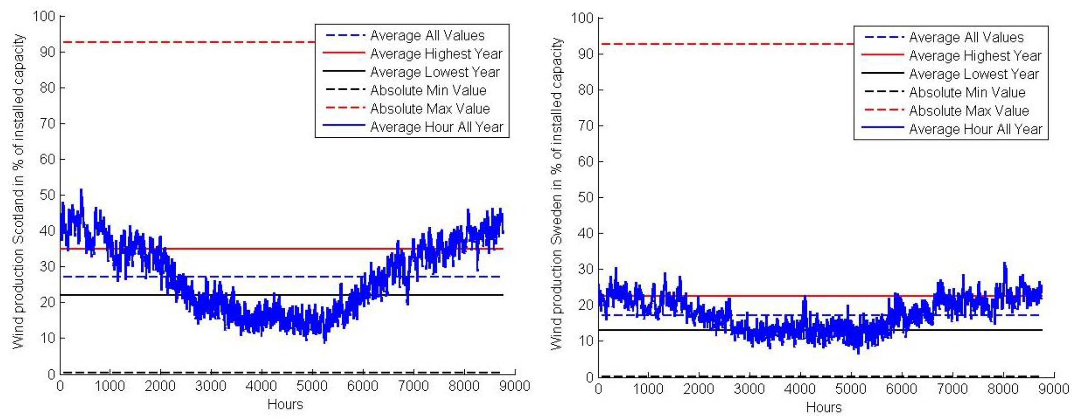
The variability characteristics have different impacts/relationships to the power system. Distribution long and short term include in our definition among other minimum and maximum values for production from aggregated wind and solar resources. The minimum value indicates the base load production that can be expected from the wind and solar resources. Looking at the net load (the difference between the load and the production from variable resources), the net load has to be supplied in all time intervals. In the present power system dis-patchable generators will balance the net load. Thus, the minimum net load value indicates the fraction of the generators capacity that must be capable of shutting off or operating at significant part load [79].
The difference between maximum and the minimum net load value indicates the minimum generator fleet power capacity that is required to meet the load demand of the system. Reserve requirements will be in addition to this value. In a future power system, energy storage and demand flexibility may balance parts of the difference between the maximum and the minimum net load value. The distribution characteristic also includes the average of the wind and solar power production. The average value gives indications for the present system how much of the total installed dis-patchable generators that are typically used over a given time period. Dis-patchable generators will in the present system over a time period balance the difference between the maximum net load and the average net load. Thus, this difference gives indications about the revenue possibility for the owners of conventional generators.
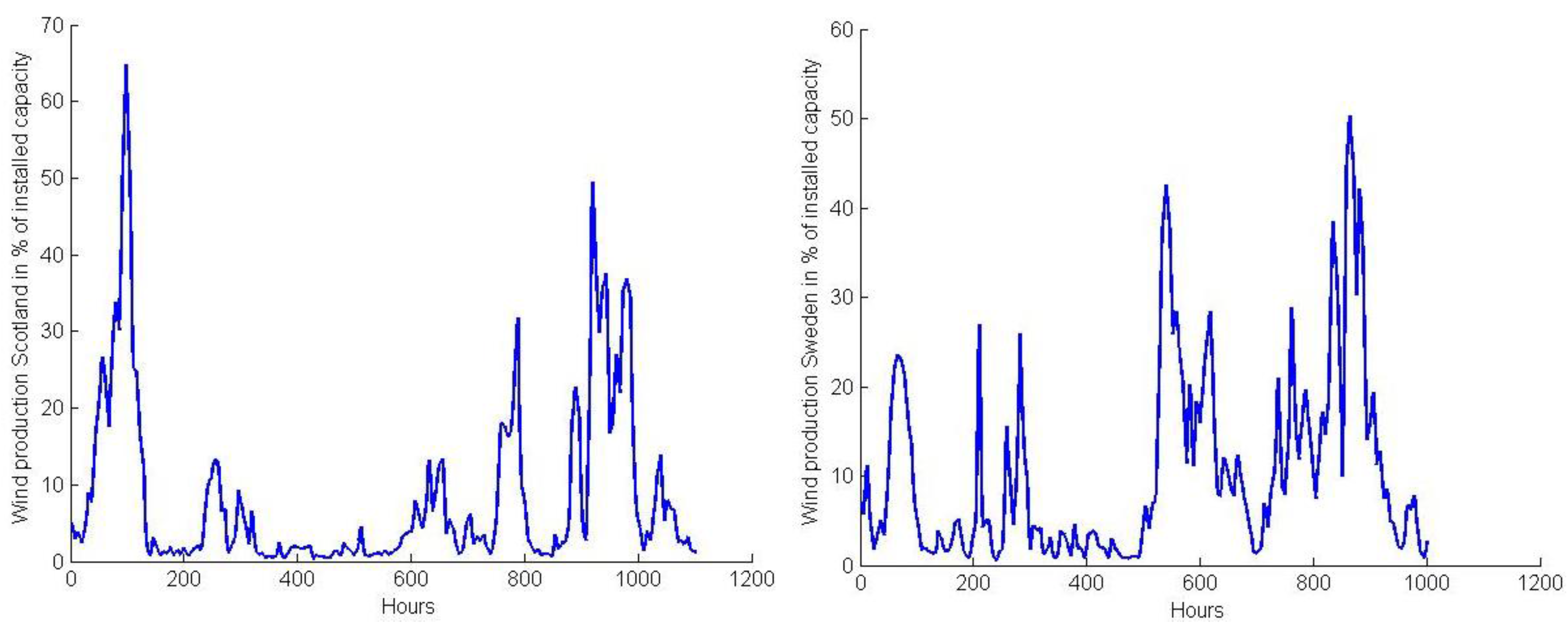
The step change characteristic gives in the present system information about how fast the conventional production have to either increase or decrease production. If storage and demand response shall balance the step changes, it gives information about expected response time and capacity of those measures. Furthermore, the frequency of the step changes gives information about how often the storage has to charge or dis-charge or how often demand has to respond to sudden increases or decreases in output from wind and solar power production plants.
The auto-correlation characteristic provides knowledge about long lasting periods with consecutive low or high net load. In the present system, the periods with low production can be balanced by dis-patchable production. In a future system with limited dis-patchable capacity left in the system, such periods may be particularly challenging. Storage technologies except for hydro-reservoirs, hydrogen and compressed air will discharge in a few hours. Furthermore, demand response will likely reduce after a few hours. Long lasting periods with surplus in the net load will result in reduced income for the owners of dis-patchable power plants as the plants have to run on part-load or shut down. Furthermore, parts of the renewable production may be curtailed, and that will lead to reduced income for the owners of the renewable production.
The characteristic predictable patterns of wind and solar resources impacts how new measures for balancing the variability match with the needs for balancing. E.g., if hydropower in Scandinavia is going to be used for balancing some of the future variability in the production in Germany, the relationship between the Predictable patterns and the yearly pattern for reservoir filling and depleting should be studied. E.g., in summer time the reservoirs are often filled up and it is not possible to pump more waters to the reservoirs even if there is surplus in the production from PV plants in Continental Europe.
The characteristics spatial correlation and cross-correlation can be utilised to smooth out production and reduce variability by connection different regions with grids.

5. Discussion and Conclusions—The Research Gap

The aim of this paper is to establish a state-of-the-art overview of the knowledge about the variability characteristics of renewable resources for the European region in a long term perspective. The review is motivated by EUs long term targets for renewable power production and also for their ambition to use demand flexibility and increased interconnectors to reduce variability challenges. By review of available scientific literature, we aim to identify the knowledge front for variability of future wind and solar power production along two dimensions:
  • How location, mix and optimal shares of wind and solar power production can contribute to smooth out the variability (correlation of resources).
  • How the aggregated wind and solar power production will vary in different time perspectives in order to be able to study how the variability can be cost-efficiently balanced by measures (demand response, different type of storage, grids) with different properties.
We structured the review in seven variable characteristics: distribution long-term (durations greater than one hour), distribution short-term (durations less than one hour), step changes, autocorrelation, spatial correlation, cross correlation and predictable patterns. This categorisation could have been organised in several ways, and there is no single correct answer to the problem. The approach proposed here represents a means of systematically subdividing a multi-faceted variability concept. Each of the characteristics is described in general terms, accompanied by a discussion of recent and relevant research related to wind power (onshore and offshore), solar power, and combined wind/solar power systems. The article focuses mainly on results from Europe, but a large number of the findings have global relevance.
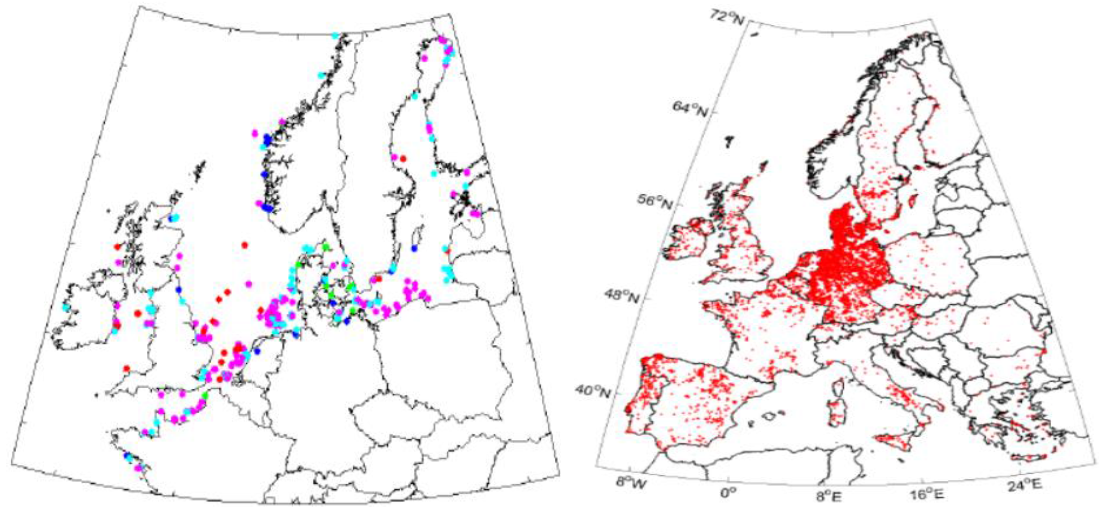
The first dimension is mainly related to the characteristics spatial correlation, cross correlation and predictable patterns. We found results confirming that the output from an integrated European power production based on solar and wind resources can be smoothed dependent on the mix and location of wind and solar resources. e.g., there is compensating trends in wind energy North and South of 45°N, so by increasing grid capacities between North and South Europe, it is probably possible to reduce variability. Source [71] showed that there is negative correlation between wind resources in e.g., Germany and Spain. The results are in accordance with source [69] which concludes that major benefits could be achieved from a more internationally renewable deployment policy providing incentives for the location of new wind farms that maximises the efficiency of overall European wind portfolios. These two studies focus only on wind power production focus. The source [33] showed that for an example of a 100% wind and solar based power production in Europe, the optimal mix of wind and solar in a seasonal perspective was 55% wind and 45% solar. However, the results in this paper are based on one specific scenario of the future portfolio and the results cannot be assumed to have general validity. All in all, we find that optimal mix and location wind and solar resources are limited studied for Europe. There are indications about possibilities for considerable reductions in variability, and we recommend that this is further investigated. It should in particular be related to EUs ambitions for increases in cross-border connection to 15% of installed electricity production capacity.
Turning to the second dimension, it can be assessed based on the four characteristics: distribution long-term, distribution short-term, step changes and autocorrelation. We found very limited results for these characteristics both on a national level and on an integrated European level for the future power system. In general, issues related to the variability of power production from onshore wind or solar resources are the subject of far more scientific papers than those related to offshore wind resources or wind and solar in combination. Furthermore, studies addressing variability in relation to a single or just a few wind or solar farms are much more common than those addressing large geographical regions, such as Europe as a whole.
EU aim to use demand response to balance some of the variability from future wind and solar power production. But since short term variations of combined wind and PV production are limited studied, it is difficult with present available knowledge to assess how the power system will be impacted if the demand side contribute with different volumes and durations of flexibility.
As mentioned in Section 1.2, for assessment of the value of the increased connection between the hydropower dominated Scandinavian system and the Germany and other neighbouring countries it is of particular interest to know how often and how long there are periods with very low production from the wind and PV based production (auto-correlation and cross-correlation). There are some results available for single countries or regions. Source [22] showed that the wind power production can be less than 5% for up to 48 h at an integrated European level. The study does not include PV production, and further studies are necessary.
In Table 12 we have indicated the impacts of the variability characteristics on the future power system and questions for further research. The list of questions does not aim to be exhaustive. The four first characteristics in the list will need to be balanced by demand response, storage, more grids or dis-patchable production and we indicate in the Table which efforts are most relevant. The research questions listed in Table 12 must be studied based on simulations of the future European power system and with different location and sizes of wind and solar power production. The simulations must include different scenarios for future load profiles. Furthermore, the simulations must include studies of possible locations of increased interconnectors between European countries given EU’s ideas of increasing cross-border connections to 15% on a case-by-case basis.
We recommend the establishment of a scheme that permits a more systematic assessment of production variability. This will promote a greater understanding of the issues at hand, and will permit a comparison of the different power production portfolios combined with different increases of interconnectors. The characteristics as proposed in this paper could constitute a starting point for such a scheme, although further work should be carried out to enable the inclusion of issues such as measures and metrics for consistent comparison.
Even though the EU is aiming to develop a future power system with very high contributions from wind and solar production, we have found only a few studies that have analysed the variability characteristics of such a system:
  • One study [32] addresses 1-h ramps in the future European power system for different contributions of wind and solar production. The study is described in Section 3.1.6.
  • One paper investigates the least-cost options for integration of intermittent renewables in low-carbon power system [11]. The investigations is based on many assumptions related to production mixes and renewable power production location, demand, demand flexibility, transmission capacities, storage, costs for technologies, fuels, CO2 etc. Western Europe is aggregated to 6 regions and one year of meteorological data is used in the simulations.
  • Two studies, [33,34], based on the same datasets, address the optimal mix of wind versus solar contributions as part of a European power system based entirely on renewable resources. The first of these studies introduces a seasonal perspective, while the other addresses energy storage capacity needs and annual balancing energy requirements and examines how hourly balancing power varies with generation capacity surpluses. These studies are also described in Section 3.1.7.
In general these studies are “snapshoots” of the future. In addition, several studies have been carried out based on the same weather conditions and system model as is applied in source [33]. These include sources [36,37,38,39,40]. These studies analyse solutions to issues caused by variability in the future European power system, but none of them include demand response. To our understanding all these studies uses the same scenario for renewable production. Thus, it is likely that the results are not valid for other development of location and mixes of wind and solar power production.
As said in the introduction to this review: “Deriving an efficient mix of integration options requires carefully analysis of power system considering the complex integration of variable renewables, other generation technologies and integration options” [12]. The variability is complex in itself and has many characteristics as shown in this study. Our final recommendation is to establish a basic understanding about this variability before it is assessed how it most cost-efficient can be balanced. By combining too many assumptions and simplifications into the same analyses, it is a possibility that opportunities are lost, e.g., hardly any study focuses on how to utilise the wind and solar resources themselves to smooth out production in a European perspective. Furthermore, by understanding the variability it is possible as proposed in the first section of this review to study how demand flexibility can balance variability in different time perspectives, instead of just assuming a certain share. This recommendation is in accordance with the recommendations in the IEA ECES26 report [16] described in Section 1.2.

Acknowledgments

The Research Council of Norway (HydroBalance project) and several Norwegian power utilities financially supported this work. Any opinions, findings, conclusions, or recommendations expressed in this paper are those of the authors and do not necessarily reflect the views of the Research Council of Norway or the Norwegian power utilities.

Author Contributions

Ingeborg Graabak is the main author of the review paper. Magnus Korpås contributed with comments and advices in the development of the paper.

Conflicts of Interest

The authors declare no conflict of interest.

Abbreviations

The following abbreviations are used in this manuscript:
CAESCompressed Air Energy Storage
CFCapacity Factor
EUEuropean Union
EVElectric Vehicles
GHGGreenhouse Gas
PVPhoto Voltaic
RESRenewable Energy Sources
TSOTransmission System Operator

References

  1. EU Energy Road Map 2050. Communication from the Commission to the European Parliament, the Council, the European Economic and Social Committee and the Committee of the Regions. Energy Road Map 2050. Brussels, 15 December 2011. Available online: http://eur-lex.europa.eu/legal-content/EN/TXT/PDF/?uri=CELEX:52011DC0885&from=EN (accessed on 1 July 2015).
  2. Renewables 2014. Global Status Report. Available online: http://www.ren21.net/Portals/0/documents/Resources/GSR/2014/GSR2014_KeyFindings_low\%20res.pdf (accessed on 1 February 2016).
  3. European Commission Press Release 25 February 2015. Available online: http://www.europa.eu/rapid/press-release_MEMO-15-4486_en.htm (accessed on 15 February 2016).
  4. Energy: New Market Design to Pave the Way for a New Deal for Consumers. Brussels, 15 July 2015. Available online: http://europa.eu/rapid/press-release_MEMO-15-5351_en.htm (accessed on 15 February 2016).
  5. German Advisory Council on Environment. Pathways towards a 100% Renewable Electricity System. Special report. Available online: http://www.umweltrat.de/SharedDocs/Downloads/EN/02_Special_Reports/2011_01__Pathways_Chapter10_ProvisionalTranslation.pdf?__blob=publicationFile (accessed on 1 April 2016).
  6. Ess, F.; Haefke, L.; Hobohm, J.; Peter, F.; Wünsch, M. The significance of international hydropower storage for the energy transistion. Prognos, October 2012. Available online: http://wec-austria.at/en/files/publikat/121023_prognos_study_international_storage_en.pdf (accessed on 1 April 2016).
  7. Hirth, L.; Ueckerdt, F.; Edenhofer, O. Integration costs revisited—An economic framework for wind and solar variability. Renew. Energy 2015, 74, 925–939. [Google Scholar] [CrossRef]
  8. Coker, P.; Barlow, J.; Cockerill, T.; Shipworth, D. Measuring significant variability characteristics: An assessment of the three UK renewables. Renew. Energy 2013, 53, 111–120. [Google Scholar] [CrossRef]
  9. Nuclear Energy Agency. Nuclear Energy and Renewables—System Effects in Low-Carbon Electricity Systems. ISBN: 978-92-64-18851. OECD, 2012. Available online: https://www.oecd-nea.org/ndd/pubs/2012/7056-system-effects (accessed on 1 February 2016).
  10. Holttinen, H.; Meibom, P.; Orths, B.; Lange, M.; O’Malley, M.; Tande, J.O.L.; Estanquerio, A.; Gomez, E.; Söder, L.; Strbac, G.; et al. Impacts of large amounts of wind power on design and operation of power systems, results of IEA collaboration. Wind Energy 2011, 14, 179–192. [Google Scholar] [CrossRef]
  11. Brouwer, A.S.; van der Broek, M.; Zappa, W.; Turkenburg, W.C.; Faaij, A. Least-cost options for integrating intermittent renewables in low-carbon power systems. Appl. Energy 2016, 161, 48–74. [Google Scholar] [CrossRef]
  12. Ueckerdt, F.; Hirth, L.; Luderer, G.; Edenhofer, O. System LCOE: What are the costs of variable renewables? Energy 2013, 63, 61–75. [Google Scholar] [CrossRef]
  13. Katzenstein, W.; Apt, J. The cost of wind power variability. Energy Policy 2012, 51, 233–243. [Google Scholar] [CrossRef]
  14. Ueckerdt, F.; Brecha, R.; Luderer, G. Analyzing major challenges of wind and solar variability in power systems. Renew. Energy 2015, 81, 1–10. [Google Scholar] [CrossRef]
  15. International Energy Agency. Technology Road Map; Energy Storage: Paris, France, 2014. [Google Scholar]
  16. Doetsch, C.; Droste-Franke, B.; Mulder, G.; Scholz, Y.; Perrin, M. Electricity Energy Storage—Future Energy Storage Demand. IEA_esec26. May 2015. Available online: http://www.iea-eces.org/files/a5.1.1_2015_eces_26_final_report_public_rev16_web.pdf (accessed on 1 April 2016).
  17. Widen, J.; Carman, N.; Carpman, N.; Castellucci, V.; Lingfors, D.; Olauson, J.; Remouit, F.; Bergkvist, M.; Grabbe, M.; Waters, R. Variability assessment and forecasting of renewables: A review for solar, wind, wave and tidal resources. Renew. Sustain. Energy Rev. 2015, 44, 356–375. [Google Scholar] [CrossRef]
  18. Buttler, A.; Dinkel, F.; Franz, S.; Spliethoff, H. Variability of wind and solar power—An assesment of the current situation in the European Union based on the year 2014. Energy 2016, 106, 147–161. [Google Scholar] [CrossRef]
  19. Van Hulle, F.; Tande, J.O.; Uhlen, K.; Warland, L.; Korpås, M.; Meibom, P.; Sørensen, P.; Morthorst, P.; Cutululis, C.; Giebel, G.; et al. Integrating Wind—Developing Europe’s Power Market for the Large-Scale Integration of Wind Power; IEE projects TradeWind, Final report; EU-project contract No. EIE/06/022/SI2.442659; EWEA: Brussels, Belgium, 2009; Available online: https://ec.europa.eu/energy/intelligent/projects/sites/iee-projects/files/projects/documents/tradewind_final_project_report_en.pdf (accessed on 1 July 2015).
  20. Tande, J.O.G.; Korpås, M.; Warland, L.; Uhlen, K.; Van Hulle, F. Impact of TradeWind offshore wind power capacity scenarios on power flows in the European HV network. In Proceedings of the 7th International Workshop on Large-Scale Integration of Wind Power and on Transmission Networks for Offshore Wind Farms, Madrid, Spain, 26–27 May 2008.
  21. Wind and radiation data. Available online: http://www.esrl.noaa.gov/psd/data/gridded/reanalysis/ (accessed on 1 April 2016).
  22. Aigner, T. System Impacts from Large-Scale Wind Power. Ph.D. Thesis, NTNU Trondheim, Trondheim, Norway, 2013. [Google Scholar]
  23. COSMO Consortium for Small-Scale Modelling. Available online: http://www.cosmo-model.org (accessed on 15 January 2015).
  24. Toornan, G.V.D.; Hassan, G.; Partners, Ltd. Tradewind, WP2: Wind Power Scenarios, W2.1-Wind Power Capacity Data Collection; Technical report; EU-project contract No. EIE/06/022/SI2.442659; EWEA: Brussels, Belgium, 2007; Available online: https://ec.europa.eu/energy/intelligent/projects/sites/iee-projects/files/projects/documents/tradewind_scenarios_of_installed_wind_capacity_en.pdf (accessed on 1 July 2015).
  25. 4coffshore, 2011. Available online: http://www.4coffshore.com/offshorewind (accessed on 1 April 2011).
  26. The Wind Power, January 2010. Available online: http://www.thewindpower.net (accessed on 1 April 2011).
  27. Energy Map. EEG-Anslagen Register, 2011. Available online: http://www.energymap.info (accessed on 1 June 2012).
  28. Bundesministerium für Umwelt, Naturschutz und Reaktorsicherheit. Gesetz für den Vorrang Erneuerbarer Energien. 2009. Available online: http://www.bmu.de/erneuerebare_energien/downloads/doc/40508.php (accessed on 1 June 2012).
  29. Drew, D.R.; Cannon, D.J.; Brayshaw, D.J.; Barlow, J.F.; Coker, P.J. The impact of Future Offshore Wind Farms on Wind Power Generation in Great Britain. Resources 2015, 4, 155–171. [Google Scholar] [CrossRef]
  30. Cannon, D.J.; Brayshaw, D.J.; Methvem, J.; Coker, P.J.; Lenaghan, D. Using reanalysis data to quantify extreme wind power generation statistics: A 33-year case study in Great Britain. Renew. Energy 2015, 75, 767–778. [Google Scholar] [CrossRef]
  31. Wiemken, E.; Beyer, H.G.; Heydenreich, W.; Kiefer, K. Power characteristics of PV ensembles, experience from the combined power production of 100 grid connected PV systems distributed over the area of Germany. Sol. Energy 2001, 70, 513–518. [Google Scholar] [CrossRef]
  32. Huber, M.; Dimkova, D. Integration of wind and solar power in Europe: Assessment of flexibility requirements. Energy 2014, 69, 236–246. [Google Scholar] [CrossRef]
  33. Heide, D.; Bremen, L.; Geriner, M.; Hoffmann, C.; Speckmann, M.; Bofinger, S. Seasonal optimal mix of wind and solar power in a future highly renewable Europe. Renew. Energy 2010, 35, 2483–2489. [Google Scholar] [CrossRef]
  34. Heide, D.; Greiner, M.; Bremen, L.V.; Hoffman, C. Reduced storage and balancing needs in a fully renewable European power system with excess wind and solar power production. Renew. Energy 2011, 36, 2515–2523. [Google Scholar] [CrossRef]
  35. Widen, J. Correlation between Large-Scale Solar and Wind Power in a Future Scenario for Sweden. IEEE Trans. Sustain. Energy 2011, 2, 177–184. [Google Scholar] [CrossRef]
  36. Andresen, G.B.; Rasmussen, M.G.; Rodriguez, R.A.; Becker, S.; Greiner, M. Fundamental properties of an transition to a fully renewable Pan-European power system. In Proceedings of the EPJ Web of Conferences, 2012; Volume 33, p. 04001. Available online: https://www.researchgate.net/publication/258643772_Fundamental_Properties_of_and_Transition_to_a_Fully_Renewable_Pan-European_Power_System (accessed on 1 October 2015).
  37. Becker, S.; Rodriguez, R.A.; Andresen, G.B.; Schramm, S.; Greiner, M. Transmission grid extension during the build-up of a fully renewable pan-European electricity supply. Energy 2014, 64, 404–418. [Google Scholar] [CrossRef]
  38. Rasmussen, M.G.; Andresen, G.B.; Greiner, M. Storage and balancing synergies in a fully or highly renewable pan-European power system. Energy Policy 2012, 51, 642–651. [Google Scholar] [CrossRef]
  39. Rodriguez, R.A.; Becker, S.; Andresen, G.B.; Heide, D.; Greiner, M. Transmission needs across a fully renewable European power system. Renew. Energy 2014, 63, 467–476. [Google Scholar] [CrossRef]
  40. Steinke, F.; Wolfrum, P.; Hoffman, C. Grid vs. Storage in a 100% Renewable Europe. Renew. Energy 2013, 50, 826–832. [Google Scholar] [CrossRef]
  41. Ackerman, T.; Söder, L. An overview of wind energy status 2002. Renew. Sustain. Energy Rev. 2002, 6, 67–128. [Google Scholar] [CrossRef]
  42. Bett, P.E.; Thornton, H.E.; Clark, R.T. European wind variability over 140 years. Adv. Sci. Res. 2013, 10, 51–58. [Google Scholar] [CrossRef]
  43. Earl, N.; Dorling, S.; Hewston, R.; Glasow, R.V. Variability in U.K. Surface Wind Climate. J. Clim. 2013, 26, 1172–1191. [Google Scholar] [CrossRef]
  44. Brayshaw, D.J.; Troccoli, A.; Fordham, R.; Methven, J. The impact of large-scale atmospheric circulation patterns on wind power generation and its potential predictability: A case study over UK. Renew. Energy 2011, 36, 2087–2096. [Google Scholar] [CrossRef]
  45. Kirchner-Bossi, N.; Garcia-Herrera, G.; Prieto, L.; Trigo, R.M. A long-term perspective of wind power output variability. Int. J. Climatol. 2015, 35. [Google Scholar] [CrossRef]
  46. Hueging, H.; Hass, R.; Born, K.; Jacob, D.; Pinto, J.G. Regional changes in wind energy potential over Europe using regional climate model ensemble projections. J. Appl. Meteorol. Climatol. 2013, 52, 903–917. [Google Scholar] [CrossRef]
  47. Holtinnen, H. Hourly Wind Power Variations in the Nordic Countries. Wind Energy 2005, 8, 173–195. [Google Scholar] [CrossRef]
  48. Held, A.M. Modelling the Future Development of Renewable Energy Technologies in the European Electricity Sector Using Agent Based Simulation. Dissertation. Stuttgart Fraunhofer, 2011. Available online: http://isbnplus.com/3839602211 (accessed on 1 September 2015).
  49. Suri, M.; Huld, T.A.; Dunlop, E.D.; Ossenbrink, H.A. Potential of solar electric generation in the European Union member states and candidate countries. Solar Energy 2007, 81, 1295–1305. [Google Scholar] [CrossRef]
  50. Wind Energy—The Facts. Part II. Grid Integration. EWEA. Available online: http://www.wind-energy-the-facts.org/images/chapter2.pdf (accessed on 1 September 2015).
  51. Sørensen, P.; Cutululis, N.A.; Vigureras-Rodriguez, A.; Madsen, H.; Pinson, P.; Jensen, L.; Hjerrild, J.; Donovan, M. Modelling of power fluctuations from large offshore wind farms. Wind Energy 2008, 11, 29–43. [Google Scholar] [CrossRef]
  52. Goic, R.; Krstulovic, J.; Jakus, D. Simulations of aggregate wind farm short-term production variations. Renew. Energy 2010, 35, 2602–2609. [Google Scholar] [CrossRef]
  53. Deane, J.P.; Drayton, G.; Gallachoir, B.P.O. The impact of sub-hourly modelling in power systems with significant levels of renewable generation. Appl. Energy 2014, 113, 152–158. [Google Scholar] [CrossRef]
  54. Ela, E.; Milligan, M.; O’Malley, M. A flexible power system operation simulation model for assessing wind integration. In Proceedings of the IEEE Power and Energy Society General Meeting, Detroit, MI, USA, 24–29 July 2011.
  55. Mills, A.; Ahlstrom, M.; Bower, M.; Ellis, A.; George, R.; Hoff, T.; Kroposki, B.; Lenox, C.; Miller, N.; Stein, J.; et al. Dark shadows: Understanding variability and uncertainty of photovoltaics for integration with the electric power system. IEEE Power Energy Mag. 2011, 3, 33–41. [Google Scholar] [CrossRef]
  56. Hoevenaars, E.J.; Crawford, C.A. Implications of temporal resolution for modelling renewables-based power systems. Renew. Energy 2012, 41, 285–293. [Google Scholar] [CrossRef]
  57. Holttinen, H.; Kiviluoma, J.; Estanquerio, A.; Gomez-Lazaro, E.; Rawn, B.; Dobschinski, J.; Meibom, P.; Lannoye, E.; Aigner, T.; Wan, Y.H.; et al. Variability of load and net load in case of large-scale distributed wind power. In Proceedings of the 10th International Workshop on Large-Scale Integration of Wind Power into Power Systems as well as on Transmission Networks for Offshore Wind farms, Aarhus, Denmark, 25–26 October 2011.
  58. Marcos, J.; Marroyo, L.; Lorenzo, E.; Alvira, D.; Izco, E. Power output fluctuations in large-scale PV plants, one year observations with one second resolution and a derived analytic model. Prog. Photovolt. Res. Appl. 2011, 19, 218–227. [Google Scholar] [CrossRef] [Green Version]
  59. Marcos, J.; Marroyo, L.; Lorenzo, E.; Garcia, M. Smoothing of PV power fluctuations by geographical dispersion. Prog. Photovolt. Res. Appl. 2012, 20, 226–237. [Google Scholar] [CrossRef] [Green Version]
  60. Santos-Alamillos, F.J.; Pozo-Vazque, Z.D.; Ruiz-Arias, J.A.; Lara-Fanego, V.; Tovar-Pescador, J. A methodology for evaluating the spatial variability of wind energy resources: Application to assess the potential contribution of wind energy to baseload. Renew. Energy 2014, 69, 147–156. [Google Scholar] [CrossRef]
  61. Oswald, J.; Raine, M.; Ashraf-Ball, H. Will British weather provide reliable electricity? Energy Policy 2008, 36, 3212–3225. [Google Scholar] [CrossRef]
  62. Østergaard, P.A. Geographic aggregation and wind power output variance in Denmark. Energy 2008, 33, 1453–1460. [Google Scholar] [CrossRef]
  63. Weigt, H. Germany’s wind energy: The potential for fossil capacity replacement and cost saving. Appl. Energy 2009, 86, 1857–1863. [Google Scholar] [CrossRef]
  64. Cassola, F.; Burlando, M.; Antonelli, M.; Ratto, C.F. Optimization of the Regional Spatial Distribution of Wind Power Plants to Minimize the Variability of Wind Energy Input into Power Supply Systems. J. Appl. Meteorol. Climatol. 2007, 46, 170–117. [Google Scholar] [CrossRef]
  65. Albadi, M.H.; El-Saadany, E.F. Overview of wind power intermittency impacts on power systems. Electr. Power Syst. Res. 2010, 80, 627–632. [Google Scholar] [CrossRef]
  66. Giebel, G. Equalizing Effects of the Wind Energy Production in Northern Europe Determined from Reanalysis Data. Riso-R 1182(EN). Roskilde, 2000. Available online: www.orbit.dtu.dk/fedora/objects/orbit:88064/datastreams/file_7729010/content (accessed on 3 May 2016).
  67. Holttinen, H. Hourly Wind Power Variation and Their Impact on the Nordic Power Operation. Ph.D. Thesis, Helsinki University of Technology, Espoo, Finland, 2003. [Google Scholar]
  68. Ernst, B. Analysis of Wind Power Ancillary Services Characteristics with German 2050 MW Wind Data. NREL Report TP-500-26969; 1999. Available online: http://www.nrel.gov/publications (accessed on 3 May 2016). [Google Scholar]
  69. Pryor, S.C.; Barthelmie, R.J.; Schoof, J.T. Inter-Annual Variability of Wind Indicies across Europe. Wind Energy 2006, 9, 27–38. [Google Scholar] [CrossRef]
  70. Reichenberg, L.; Johnsson, F.; Odenberger, M. Dampening variations in wind power generation—The effect of optimizing geographic location of generation sites. Wind Energy 2014, 17, 1631–1643. [Google Scholar] [CrossRef]
  71. Roques, F. Optimal wind power deployment in Europe—A portfolio approach. Energy Policy 2010, 38, 3245–3256. [Google Scholar] [CrossRef]
  72. Perez, R.; Hoff, T.E. Chapter 6—Solar resource variability. In Solar Energy Forecasting and Resource Assessment; Kleissl, J., Ed.; Academic Press: Boston, MA, USA, 2013; pp. 133–148. [Google Scholar]
  73. Perez, R.; Kivalov, S.; Schlemmer, J.; Hemker, K., Jr.; Hoff, T.E. Short-term irradiance variability: Preliminary estimation of station pair correlation as a function of distance. Sol. Energy 2012, 86, 2170–2176. [Google Scholar] [CrossRef]
  74. Hinkelman, L.M. Differences between along-wind and cross-wind solar irradiance variability on small spatial scales. Sol. Energy 2013, 88, 192–203. [Google Scholar] [CrossRef]
  75. Santos-Alamillos, F.J.; Pozo-Vazquez, J.A.; Ruiz-Arias, J.A.; Lara-Fanego, V.; Tovar-Psecador, J. Analysis of Spatiotemporal Balancing between Wind and Solar Energy Resources in the Southern Iberian Peninsula. J. Appl. Meteorol. Climatol. 2012, 51, 2005–2024. [Google Scholar] [CrossRef]
  76. Hoicka, C.E.; Rowland, I.H. Solar and wind resource complementary: Advancing options for renewable electricity integration in Ontario, Canada. Renew. Energy 2011, 36, 97–107. [Google Scholar] [CrossRef]
  77. Montfori, F.; Huld, T.; Bodis, K.; Vitali, L.; D’Isidoro, M.; Lacal-Arántegui, R. Assessing complementary of wind and solar resources for energy production in Italy. A Monte Carlo approach. Renew. Energy 2014, 63, 576–586. [Google Scholar]
  78. Liu, Y.; Xiao, L.; Wang, H.; Dai, S.; Qi, Z. Analysis of the spatiotemporal complementarities between China’s solar and wind resources spreading in a wide area. Sci. China Technol. Sci. 2013, 56, 683–692. [Google Scholar] [CrossRef]
  79. Tarroja, B.; Mueller, F.; Eichman, J.D.; Samuelsen, S. Metrics for evaluating the impacts of intermittent renewable generation on utility load-balancing. Energy 2012, 42, 546–562. [Google Scholar] [CrossRef]
Figure 1. Left: wind farms in the North and Baltic Seas in 2030 (colour code—installed capacity (MW): blue <10, green 10–80, cyan 80–200, magenta 200–800, red >800). Right: locations of European onshore wind installations [22]. Reproduced with permission from T. Aigner.
Energies 09 00449 g001
Figure 2. Illustration of Distribution Long-Term for Scotland and northern Sweden (described in Section 3.1.1).
Energies 09 00449 g002
Figure 3. Annual full load hours of optimally inclined PV modules (see [48]), based on data from source [49] and a performance ratio of 0.75. Reproduced with permission from A. Held.
Energies 09 00449 g003
Figure 4. Step changes in wind power production in Scotland and in northern Sweden (study described in Section 3.1.1).
Energies 09 00449 g004
Figure 5. Example of autocorrelation for wind speed (left) and solar irradiance (right) [8]. Reproduced with permission from P. Coker.
Energies 09 00449 g005
Figure 6. Periods of persistent production below 5% for Scotland and northern Sweden (study described in Section 3.1.1).
Energies 09 00449 g006
Figure 7. Spatial wind correlation between northern (blue curve) and southern (red) Sweden, displayed together with an aggregated curve (black) for a selected year (study described in Section 3.1.1).
Energies 09 00449 g007
Figure 8. Predictable yearly patterns of wind power production in terms of per cent of installed capacity for Scotland (to the right) and northern Sweden (to the left) (study described in Section 3.1.1).
Energies 09 00449 g008
Table 1. Nodes used in the illustrations of wind variability characteristics.
Name of NodeLatitudeLongitudeAdj. Factor
Sweden01 (north)66.020.01.12
Sweden04 (south)56.515.01.12
Scotland56.6−4.00.91
Table 2. Wind power installation scenarios [22].
(GW)20102030
CountryOnshoreOffshoreOnshoreOffshore
Germany25.30.133.924.1
The Netherlands2.60.23.912.8
United Kingdom9.71.333.526.2
Europe88.82.4292.6104.4
Table 3. Annual wind power generation expressed in percentage of installed capacity for wind speeds recorded in 2010 and 2011 (in brackets) [22].
(%)EuropeNorth and Baltic Sea
2010203020102030
Min1.6 (2.4)2.5 (3.0)0.4 (0.6)1.5 (1.8)
Mean16.6 (18.1)18.6 (20.1)17.6 (21.8)28.6 (33.5)
Max56.2 (59.7)60.1 (62.2)77.2 (81.1)86.8 (92.1)
Table 4. Hourly variation in wind power production for a single site and the Nordic region for the years 2000–2002 [47]. St. dev.: standard deviation.
(%)Single SiteNordic Region
Mean25.925.1
Median14.922.4
St. dev.28.214.5
Min0.01.2
Max105.086.5
Table 5. Hourly balancing quintiles for different combinations of wind and solar PV in a 100% wind/solar-based European power system [34].
Balancing Quintiles
aq = 0.9q = 0.99q = 0.999
0.60.5540.8070.973
0.70.5010.7590.931
0.80.4650.7180.899
0.90.4790.7080.877
Table 6. Mean and maximum values, standard deviation and hourly ramps for a combined case involving a combined total of 10 TWh/year from solar and wind production in Sweden [35]. (Std. dev.: standard deviation).
Annual Production (TWh)Combined Output P (GW)Hourly Change|∆P| (GW)
SolarWindMeanMaxStd. devMeanMaxStd. dev.
1001.147.971.720.313.230.42
911.147.181.540.282.900.37
821.146.461.350.252.570.33
731.145.811.180.222.250.29
641.145.231.030.191.920.25
551.144.750.890.171.590.20
461.144.450.800.141.300.16
371.144.260.750.111.000.12
281.144.080.760.090.710.08
191.143.890.820.060.710.06
0101.143.910.930.050.790.05
Table 7. Maximum downward and upward hourly ramping for wind power generation as a percentage of installed capacity [22].
(%)EuropeNorth and Baltic Sea
2010203020102030
Max down−7.2−6.6−0.1−9.2
Max up5.26.00.110.7
Table 8. 1-h net load ramps [share of peak load] mean of 27 countries and their statistical dispersion [32].
αβMeanMinMaxStd. Dev
99th Percentile
0.30.20.10.070.160.02
0.40.120.090.150.02
0.60.150.120.190.02
0.50.20.130.090.190.03
0.40.180.130.220.02
0.60.260.20.30.03
1st Percentile
0.30.2−0.08−0.13−0.050.02
0.4−0.1−0.14−0.070.02
0.6−0.13−0.19−0.080.02
0.50.2−0.11−0.2−0.080.03
0.4−0.16−0.23−0.10.03
0.6−0.23−0.32−0.150.04
Table 9. Frequency of persistently low and high availability events derived from a MERRA reanalysis [30].
Event TypeThresholdsMean YearMin YearMax Year
Persistent lowCF ≤ 6.3%10218
Persistent highCF ≥ 69.9%12427
Table 10. Wind power mean and standard deviation data, and correlation coefficients for five European countries [71].
SpainGermanyAustriaDenmarkFrance
Mean0.2290.1950.2290.2420.214
Standard dev.0.1380.1720.2130.2180.137
Cross correlation
Spain1.00−0.0330.011−0.0610.062
Germany 1.000.0450.3620.147
Austria 1.0000.0050.010
Denmark 1.0000.046
France 1.000
Table 11. Overview of wind and solar variability characteristics and the European knowledge front for each characteristic.
Characteristic NameKnowledge Front
Description/Definition
Distribution Long-TermFew large-scale studies include both onshore and offshore wind and solar power. We did to find any published results about yearly variation in combined wind/solar production systems. For most onshore wind power production sites, the annual capacity factor is 20%–40% while offshore wind reaches 45%–57%. A large-scale wind power study covering all of Europe produced the following values (figures are in percentage of installed capacity): mean = approx. 20%, min. value = approx. 3%, max. value = approx. 60%, wind power below 10% approx. 1000 h/year, wind power above 50% approx. 600 h/year). Studies showed significant differences between annual wind speed data sets covering Europe. The regions most affected by annual variations include the main projected construction sites for future offshore wind farms [22]. Full load hours for optimal inclined PV production in Europe are in the range 650 to 1500 h/year.
Distribution of discrete energy outputs over defined time periods (hours to years) assessed over a longer duration of time
Distribution Short-TermFew large-scale studies exist that address wind variability, either onshore or offshore, with resolutions in the range 15 to 60 min. No result is found regarding the short-term distribution for large-scale wind and solar power production in combination.
Distribution of discrete energy outputs over defined time periods (less than an hour) assessed over a longer duration of time
Step ChangesAccording to simulations [22], the maximum hourly fluctuations of large-scale wind power production in a future Europe is about ±6%–7% of installed capacities. The most significant variations are the result of passing storm fronts, during which wind turbines reach their storm limit (cut-out wind speed) and shut down rapidly from full to zero power. A relative increase in the contribution from offshore wind will increase Step Changes due to the density of offshore wind production sites in the North Sea, and the presence of lower smoothing effect offshore than onshore. Another study [32] found that a contribution from solar of more than 20%–30% as a percentage of renewable power production in a future scenario will have a considerable effect on 1-h ramps. The study did not consider offshore wind power production. For European countries, the highest hourly solar PV ramps are measured at up to 18%–25% of capacity.
Changes in energy outputs over different time intervals
AutocorrelationWe failed to find a study addressing persistent high and low production levels from a system based on both solar and wind resources. Source [22] indicates that future wind power production in Europe could be less than 5% for durations of up to 48 h. One study [29] investigated persistent high and low wind generation for current and future wind power production in the UK, and revealed that there is large inter-annual variability in the frequency of persistent events. One might expect fewer persistent low generation events, and more persistent high generation events in scenarios where the contributions from offshore wind are high. If production is persistent above a certain level, this level could be considered as the base-load supply. There are only a few studies available dealing with base load supply from wind power production in Europe, and no studies at all for combined wind and solar power production systems. According to [18] the aggregated wind power production in the European power system in 2014 never was below 5% of installed capacity and never was below 9% in the period December–February.
The existence of statistical dependence among successive values of the same variable
Spatial CorrelationThere is a high degree of covariance between wind indices in northern Europe [69]. The axis about which the correlations of latitudinal integrated wind indices over Europe changes sign is approximately 45°N (between the Caspian Sea coast of the Russian Caucasus in the east and the Bay of Biscay in the west). There is also evidence of compensating trends in wind energy indices north and south of this latitude. One study found a reduction in wind power variability of 33% in the event of the optimal location of wind power sites in northern Europe [70].
Correlation between resource mixes of the same type (e.g., wind- wind or solar-solar)
Cross CorrelationTo date, research into the smoothing effects from the combination of wind and solar power production has been only limited studied. Studies demonstrate a negative correlation between solar and wind production, especially on monthly/seasonal scales. According to one study, power production variability can be decreased significantly by the optimal location of wind and solar production sites based on the correlation between these resources [75].
Correlation between different types of RES, e.g., wind, solar
Predictable PatternsAccording to a data set for the period 2000–2002 [47], there is a distinct seasonal variation in wind power production in central and northern Europe. In winter, production is greater (110%–150% of yearly average) than in summer (60%–80%). In Europe as a whole, there is a tendency for wind speeds to increase in the morning and to calm down in the evening. In northern Europe, this phenomenon is more pronounced in summer.
Predictable resource availability patterns dependent on geographical location.
Table 12. The variability characteristics, their relations to the power future system and suggestions for further research.
Variability CharacteristicConsequences/Possibilities for the Power SystemSuggestions for Further Research
Distribution Long TermVariation between a few hours of limited size can probably be balances by demand response, short term storage and more grids. For long lasting or frequent periods with low production from the wind and solar power plants, more interconnector may reduce the variability. Hydro power production in Scandinavia may contribute to smooth out long periods with very low or very high production.
  • What is the size and the duration of the variations that can be expected in the time perspective an hour or more if new wind and solar power production are optimally distributed according to the characteristics Spatial correlation, Cross-correlation and Predictable patters and the interconnectors are optimally increased in order to reduce long term variability?
  • Where is it most appropriate to increase interconnectors to smooth out variations over longer term?
  • To which extent can Scandinavian hydropower contribute?
Distribution Short TermA large share of the variations within an hour can probably be balance by demand response (if the consumer is given appropriate incentives) and by increased storage. Furthermore, more interconnector can contribute to smooth out short term variations.
  • What is the size of variations which can be expected within an hour?
  • Where is it most appropriate to increase interconnectors to smooth out Short Term variations?
  • Can all Short Term variations be balanced with demand response, storage and increased interconnectors? If not, what is the remaining share?
Step ChangesDependent on the size of the Step Changes, demand response, storage and more interconnectors can reduce the impacts of Step Changes
  • What is the size of the largest Step changes that can be expected for different time intervals?
  • How frequently and at which time of the year do these Step Changes occur?
  • Where is it most appropriate to increase interconnectors to reduce the largest Step Changes?
  • Can all Step Changes be balanced with demand response, storage and increased interconnectors? If not, what is the remaining share?
Auto-CorrelationPeriods over several days to weeks with low production from wind and solar can probably not be balanced with demand response. Except for large-scale hydro reservoirs, present available storage technologies will not be able to balance long lasting low production periods. Interconnectors may reduce the effect of auto-correlation
  • What is the expected size and duration of the low production periods after increasing the most appropriate interconnectors?
  • How frequently and when (summer/winter) do they occur?
  • Where is it most appropriate to increase interconnectors in order to reduce long lasting periods with low production?
Spatial Correlation/Cross correlation/Predictable/PatternsCan be used to reduce variability and can be particularly important for smoothing out long and frequent periods with low production
  • What is the optimal location and size of wind power production and for solar power production to utilize Spatial Correlation/Cross Correlation/Predictable Patterns to smooth out variability?
  • Where is it most appropriate to increase interconnectors to utilise the Spatial Correlation/Cross Correlation/Predictable Patterns effects?

