Thermo-Economic and Heat Transfer Optimization of Working-Fluid Mixtures in a Low-Temperature Organic Rankine Cycle System ^†

Abstract

In the present paper, we consider the employment of working-fluid mixtures in organic Rankine cycle (ORC) systems with respect to thermodynamic and heat-transfer performance, component sizing and capital costs. The selected working-fluid mixtures promise reduced exergy losses due to their non-isothermal phase-change behaviour, and thus improved cycle efficiencies and power outputs over their respective pure-fluid components. A multi-objective cost-power optimization of a specific low-temperature ORC system (operating with geothermal water at 98 °C) reveals that the use of working-fluid-mixtures does indeed show a thermodynamic improvement over the pure-fluids. At the same time, heat transfer and cost analyses, however, suggest that it also requires larger evaporators, condensers and expanders; thus, the resulting ORC systems are also associated with higher costs. In particular, 50% n-pentane + 50% n-hexane and 60% R-245fa + 40% R-227ea mixtures lead to the thermodynamically optimal cycles, whereas pure n-pentane and pure R-245fa have lower plant costs, both estimated as having ∼14% lower costs per unit power output compared to the thermodynamically optimal mixtures. These conclusions highlight the importance of using system cost minimization as a design objective for ORC plants.

1. Introduction

Organic Rankine cycle (ORC) power systems are a relatively mature, commercially available technology, that is highly appropriate for the conversion of heat at temperatures below ∼300–400 ${}^{\circ }$C to useful work at power-output scales from a kW to tens of MW [1]. The selection of working fluids for ORC systems has received attention recently, including a particular interest in multi-component fluid mixtures, due to the opportunities they offer in improving thermodynamic performance. Various authors have performed investigations to demonstrate and quantify these benefits, which have shown that fluid mixtures and pure fluids at supercritical pressures can achieve an improved thermal match with the heat source (i.e., a reduced average temperature-difference) compared to the isothermal profile of the (isobaric, sub-critical) evaporation of pure-component fluids, thereby reducing exergy losses due to heat transfer, and increasing thermal and exergy efficiencies [2,3,4,5,6].

Both experimental and theoretical studies have been performed into the benefits of employing refrigerant [7,8,9,10], hydrocarbon [11,12] and siloxane [13,14] fluid mixtures, over a range of heat-source temperatures. Compared to pure fluids, binary mixtures have shown increased power outputs by up to 30% and thermal efficiencies by over 15% in some cases. Excellent second law analyses have also shown significant potential benefits [15,16,17]. These benefits are especially magnified in applications with limited cooling-water supply, e.g., combined heat and power (CHP) systems where the non-isothermal temperature profiles of the condensing fluid mixtures provide a good thermal match to the temperature profile of the heated cooling stream [5]. However, some exceptions to these general trends have also been reported [5,18], especially in cases where there is an adequate supply of a cooling stream, limiting the benefits accruable to employing working-fluid mixtures. Additionally, mixtures can be used to adjust the environmental and safety-related properties of ORC working fluids or to improve design parameters of system components. At the same time, some investigators have begun to develop and apply advanced computer-aided molecular design (CAMD) methodologies [19,20,21,22] with a view towards identifying or designing optimal fluids for ORC applications.

While these efforts have demonstrated the potential advantages of working-fluid mixtures, notably in terms of power output and efficiency, many of the associated conclusions have been derived strictly based on thermodynamic cycle analyses that do not fully consider the expected heat transfer performance between the heat source/sink and working-fluid streams in the heat exchangers of ORC engines. In particular, the heat transfer and (importantly) the cost implications of using working-fluid mixtures have not been properly addressed and are in need of further consideration. Refrigerant mixtures are known to exhibit reduced heat-transfer coefficients (HTCs) compared to their pure counterparts [23,24,25,26,27,28,29]. Specifically, HTCs for refrigerant mixtures are usually lower than the ‘ideal’ values, linearly interpolated between the mixture components [30,31,32,33]. This, coupled with the reduced temperature difference between the heat source/sink (wherever this applies) and the working-fluid mixture, will invariably lead to larger and more expensive heat exchangers in an ORC system. Therefore, although working-fluid mixtures may allow a thermodynamic advantage over single-component working fluids, they may also lead to higher system costs owing to a deterioration in their thermal performance and increased component size.

This deterioration in the HTCs of working-fluid mixtures, especially during the phase change processes, is ordinarily not accounted for with simple HTC correlations developed for pure fluids or those developed using (averaged/weighted) thermodynamic properties of the mixtures. Thus, and, by extension, the overall effect of these working-fluid mixtures on the ORC system components’ (heat exchangers, expanders and pumps) sizes and costs will not be adequately accounted for by these HTC models or by simple cost functions that are based on aggregated properties of ORC systems such as heat-exchanger duties or power output. Therefore, there is the need to go beyond these efforts in order to qualify the precise effect of working-fluid mixtures against their pure counterparts, on the design and economics of ORC plants. The reduced heat transfer performance of the fluid mixtures needs to be expressly accounted for, including the subsequent effect on the exact (physical) sizes (e.g., areas of heat exchangers, and volumes of expanders and pumps) and costs of the individual components of the ORC system, leading to a well-defined analysis of the benefits and drawbacks of employing working-fluids mixtures (in comparison with pure working fluids) in ORC systems.

By presenting a method for evaluating the HTCs of working-fluid mixtures, this work aims to explore the effects of using such mixtures on the overall heat transfer processes and component sizing in ORC engines, which are important in understanding the role that these fluids play on the overall system performance and cost. A simple ORC engine model is presented that incorporates a suitable heat transfer description of the heat exchangers used for the heat addition and heat rejection processes. The heat exchangers are discretized along their lengths into segments (accounting for phase-change and single-phase regions), with suitable estimates of the HTCs in the different segments. Overall HTCs and heat-transfer areas (HTAs) are then evaluated for the ORC system heat exchangers. Furthermore, the expanders and working-fluid pumps are sized based on their power requirements as their sizes are also affected by the working-fluid selection. Simple cost models are then used to estimate the relative costs of the components, and, by extension, of the entire engine. Using a selection of alkane and refrigerant working-fluid mixtures, the heat transfer characteristics and ORC-system equipment/component costs are thus investigated.

2. Models and Methodology

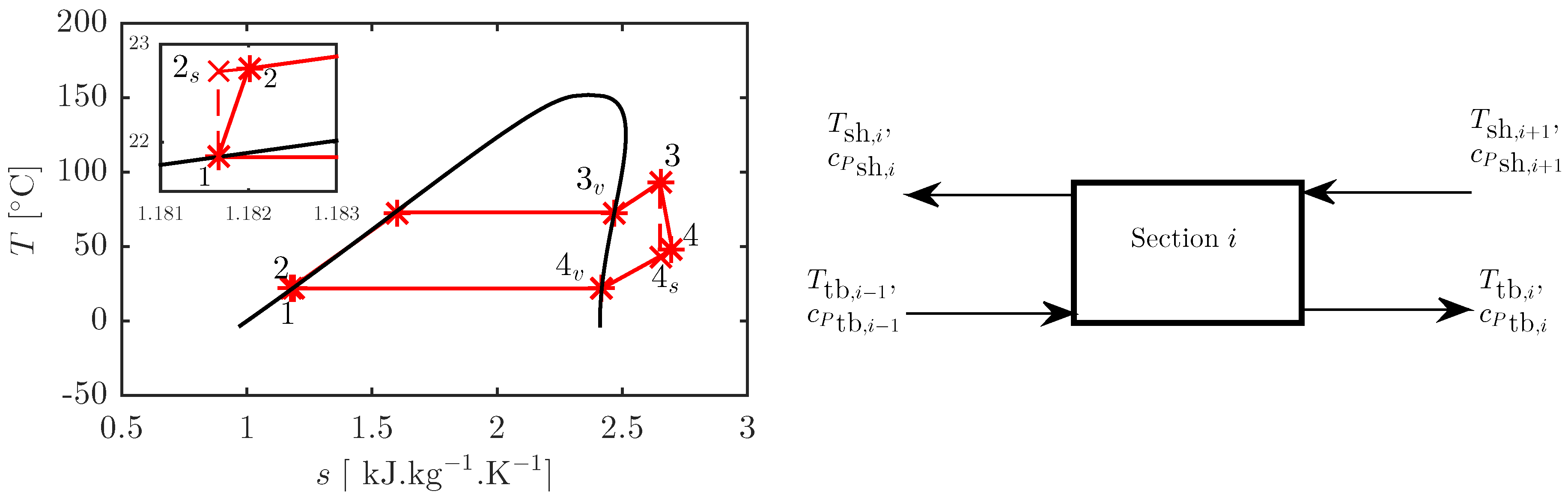
2.1. ORC Thermodynamic Model

We consider a sub-critical, non-regenerative ORC consisting of four basic processes (pumping, heat addition, expansion and heat rejection), carried out by an organic working fluid (wf). A typical such ORC is presented in the T–s diagram in Figure 1. Briefly, for completeness, the power required to pump the working fluid from State 1 (saturated liquid) to State 2 is:

$${\dot{W}}_{\mathrm{pump}}={\dot{m}}_{\mathrm{wf}}(h_2-h_1)={\dot{m}}_{\mathrm{wf}}(h_{\mathrm{2s}}-h_1)/{\eta }_{\mathrm{is,pump}}.$$

(1)

The heat extracted from the heat source is transferred to the working fluid assuming no heat losses and no pressure losses, i.e., an isobaric heat-addition process. In order to study the role of superheating on the thermo-economic performance of the ORC systems considered here, the working fluid is allowed to exit the heat-addition process either as a saturated vapour (State $3_v$, with no superheating) or as a superheated vapour (State 3), even though it has been reported that superheating may be detrimental to thermodynamic performance of ORC systems [34]. Specifically, the working fluid is allowed to exit the process with varying levels of superheat in order to quantify the optimal degree of superheating for the different working fluids. For convenience, in varying this parameter, we define a normalized (and dimensionless) degree of superheating ($d_{\mathrm{SH}}$, which varies between 0 and 1 irrespective of the fluid, cycle and the external conditions), as opposed to a fixed value (e.g., 5 ${}^{\circ }$C or 10 ${}^{\circ }$C) above the dew-point temperature, as:

$$d_{\mathrm{SH}}=\frac{T_3-T_{\mathrm{dew}}(P_{\mathrm{evap}})}{T_{\mathrm{hs,in}}-\Delta T_{\min }-T_{\mathrm{dew}}(P_{\mathrm{evap}})}.$$

(2)

Thus, the rate of heat input from the heat source (hs) is given by:

$${\dot{Q}}_{\mathrm{in}}={\dot{m}}_{\mathrm{hs}}{c}_{p,\mathrm{hs}}(T_{\mathrm{hs,in}}-T_{\mathrm{hs,out}});\mathrm{and,}{\dot{Q}}_{\mathrm{in}}={\dot{m}}_{\mathrm{wf}}(h_3-h_2).$$

(3)

Following the heat-addition process, the power generated as the working fluid is expanded to State 4 is:

$${\dot{W}}_{\exp }={\dot{m}}_{\mathrm{wf}}(h_3-h_4)={\eta }_{\mathrm{is,exp}}{\dot{m}}_{\mathrm{wf}}(h_3-h_{\mathrm{4s}}).$$

(4)

After expansion, the working fluid rejects heat to the cooling stream. During heat rejection, the working fluid transfers heat to a cooling stream (cs) at a rate given by:

$${\dot{Q}}_{\mathrm{out}}={\dot{m}}_{\mathrm{wf}}(h_4-h_1);\mathrm{and,}{\dot{Q}}_{\mathrm{out}}={\dot{m}}_{\mathrm{cs}}{c}_{p,\mathrm{cs}}(T_{\mathrm{cs,out}}-T_{\mathrm{cs,in}}).$$

(5)

The pump and expander isentropic efficiencies (${\eta }_{\mathrm{is,pump}}$ and ${\eta }_{\mathrm{is,exp}}$) are taken as 75%, while all necessary fluid properties are calculated with REFPROP 9.1 [35,36]. The thermal efficiency of the cycle is calculated as:

$${\eta }_{\mathrm{th}}={\displaystyle \frac{{\dot{W}}_{\mathrm{net}}}{{\dot{Q}}_{\mathrm{in}}}}={\displaystyle \frac{{\dot{W}}_{\exp }-{\dot{W}}_{\mathrm{pump}}}{{\dot{Q}}_{\mathrm{in}}}}.$$

(6)

2.2. Heat Exchanger Sizing

The heat addition process is carried out in two heat exchangers: (1) the Preheater (PH), used to pre-heat the working fluid to saturated liquid; and (2) the Evaporator (Ev), used to evaporate the working fluid to the saturated vapour state and to also superheat the working fluid when necessary. Similarly, the heat rejection process is carried out in the Desuperheater (DSh) and the Condenser (Cn). The heat exchangers are modelled as counter-current, double-pipe heat exchangers with standard/nominal shell and tube sizes of 6 in and 4 in (for PH and Ev), and 8 in and 6 in (for DSh and Cn), respectively. The sizes are selected to provide turbulent flow regimes, while maintaining reasonably low flow velocities in both the shell and tube sides of the heat exchangers.

The heat exchangers are assumed to be constructed from carbon-steel (thermal conductivity: k = 51 W·m^-1·K^-1), and are discretized (for modelling purposes) into 100 (variable-sized) segments, i (=1–100), each segment having an equal heat transfer/duty, i.e., ${\dot{Q}}_{\mathrm{in}}/100$ or ${\dot{Q}}_{\mathrm{out}}/100$. A typical segment is illustrated in Figure 1. In all heat exchangers, the working fluid flows through the tube-side (tb), while the heat source and sink streams are the shell-side (sh) fluids. Thus, the total rates at which heat is transferred to/from the working fluid in relation to Equations (3) and (5), respectively, are given by:

$${\dot{Q}}_{\mathrm{in}}={\dot{Q}}_{\mathrm{PH}}+{\dot{Q}}_{\mathrm{Ev}}=\sum _{i=1}^{100}{\dot{Q}}_{\mathrm{PH},i}+\sum _{i=1}^{100}{\dot{Q}}_{\mathrm{Ev},i};\mathrm{and,}{\dot{Q}}_{\mathrm{out}}={\dot{Q}}_{\mathrm{DSh}}+{\dot{Q}}_{\mathrm{Cn}}=\sum _{i=1}^{100}{\dot{Q}}_{\mathrm{Dsh},i}+\sum _{i=1}^{100}{\dot{Q}}_{\mathrm{Cn},i}.$$

(7)

Furthermore, for each segment an overall heat-transfer coefficient, $U_i$, can be defined such that:

$${\dot{Q}}_i=U_i{A}_i\Delta T_{\mathrm{lm},i},\text{where}:$$

(8)

$$\Delta T_{\mathrm{lm},i}={\displaystyle \frac{(T_{\mathrm{sh},i+1}-T_{\mathrm{tb},i})-(T_{\mathrm{sh},i}-T_{\mathrm{tb},i-1})}{\ln [(T_{\mathrm{sh},i+1}-T_{\mathrm{tb},i})/(T_{\mathrm{sh},i}-T_{\mathrm{tb},i-1})]}};\mathrm{and,}{U_i}^{-1}={h_{\mathrm{sh},i}}^{-1}+dx/k+{h_{\mathrm{tb},i}}^{-1}.$$

(9)

Single-phase local HTCs ($h_{\mathrm{sh}}$, $h_{\mathrm{tb}}$) can be calculated by using the Dittus–Boelter Nusselt number (${\mathrm{Nu}}_{i,\mathrm{sp}}$) correlation, whereas two-phase HTCs can be calculated by suitably modifying ${\mathrm{Nu}}_{i,\mathrm{sp}}$ with empirical functions of the Martinelli parameter, $X_{\mathrm{tt}}$ [23,37]. In the present work, this modification was fitted specifically to results from experiments involving horizontal turbulent-flow boiling of refrigerant mixtures as:

$${\mathrm{Nu}}_{i,\mathrm{tp}}=\mathrm{F}(X_{\mathrm{tt}}){\mathrm{Nu}}_{i,\mathrm{sp}},\text{where}\mathrm{F}(X_{\mathrm{tt}})=1+1.8{X_{\mathrm{tt}}}^{-0.82},\text{and}{X}_{\mathrm{tt}}={\left({\displaystyle \frac{1-q}{q}}\right)}^{0.9}{\left({\displaystyle \frac{{\rho }_{\mathrm{v}}}{{\rho }_{\mathrm{l}}}}\right)}^{0.5}{\left({\displaystyle \frac{{\mu }_{\mathrm{l}}}{{\mu }_{\mathrm{v}}}}\right)}^{0.1}.$$

(10)

Equation (10) can be applied directly for pure fluids using the overall mixture composition for the liquid and vapour-phase properties. For the fluid mixtures, $X_{\mathrm{tt}}$ is calculated using the equilibrium liquid and vapour-phase compositions (not the overall composition) at the saturation temperature and corresponding vapour quality, q, on mass basis [23]. The HTAs of all segments are then calculated from Equation (8) and summed to give the total HTA ($A_{\mathrm{HX}}$) for the heat exchanger of interest.

2.3. Component Cost Estimation

The key components affected by the choice of working fluid are those illustrated previously—the working-fluid pump, the expander and the heat exchangers. The costs of these components are added to give an estimate of the plant cost. Although this sum does not give the total installation cost, it is through this amount that the effects of working-fluid choice on plant costs are manifested directly. Other factors that contribute to the plant installation costs would be similar for the various working fluids, considered especially as the fluids considered in this work are of the same chemical class; other factors such as flammability and corrosiveness can increase investment costs when comparing working fluids from different chemical classes.

Generally, there are uncertainties inherent in the estimation of costs of process equipment and plants (and also in the estimation of heat-transfer coefficients, albeit to a lesser degree), with preliminary cost estimation techniques being accurate up to $\pm 25\%$ [38,39]. While these uncertainties do exist, the qualitative information derived from using a particular costing technique for comparison of plants/systems of different sizes will not be influenced to a large degree by such uncertainties. Thus, it is important to use a single and consistent source of information for the comparison of the ORC systems employing different working fluids.

Various techniques are available for estimating the installation/capital costs of process equipment and units. Data for such techniques are usually obtained from surveys of equipment manufacturers during a particular time period. An example is the capital equipment-costing (CAPCOST) program [38] which contains the capital costs of a large variety of process equipment, benchmarked in the year 2001. Another technique available is the C-value method, used in combination with the ESDU 92013 chart [40], produced in 1994, for estimating the cost of different types of heat exchangers. Similar to the CAPCOST program, logarithmic correlations are presented for a wide range of process equipment in Seider et al. [39]; the data used for these correlations were gathered in the year 2006. Generally, conversions from the publication years (1994, 2001 or 2006) to the current year can be carried out using the Chemical Engineering Plant Cost Index (CEPCI).

In this work, we employ the correlations provided by Seider et al. [39] due to its more recent date of production, thereby minimizing variations introduced by year-to-year conversions with the CEPCI. Component-base costs ($C_{\mathrm{B}}$, indexed in year 2006; £1 ≡ €1.47, $1.84) are calculated using logarithmic correlations of component size factors (S) according to Seider et al. [39]:

$$C_{\mathrm{B}}=(F)exp\{C_0+C_1[\ln S]+C_2{[\ln S]}^2\}.$$

(11)

The component size factors are presented in

Table 1. Component cost coefficients used in Equation (11).

Component	S	F	${\mathit{C}}_{\mathbf{0}}$	${\mathit{C}}_{\mathbf{1}}$	${\mathit{C}}_{\mathbf{2}}$
Pump	$\dot{V}\sqrt{H}$ (m3·s−1·m1/2)	2.7	9.0073	0.4636	0.0519
Expander	${\dot{W}}_{\exp }$ (kW)	1.0	6.5106	0.8100	0.0000
Expander *	${\dot{W}}_{\exp }$ (kW)	1.0	7.3194	0.8100	0.0000
Heaters/Coolers	HTA (m2)	1.0	10.106	−0.4429	0.0901
Evaporator/Condenser	HTA (m2)	1.0	9.5638	0.5320	−0.0002

* Sub-atmospheric pressure (vacuum) discharge expander (applicable for $x_{{\mathrm{C}}_6{\mathrm{H}}_{14}}\ge 0.1$).

. Also provided in Table 1 are the cost coefficients ($C_0$, $C_1$, $C_2$, converted to SI units). The correlation for the pump motor (with ${\dot{W}}_{\mathrm{pump}}$ re-expressed in units of hp) base cost contains more terms and is given by (to 3 significant figures):

$$C_{\mathrm{B}}=exp\{5.83+0.134[\ln {\dot{W}}_{\mathrm{pump}}]+0.0533{[\ln {\dot{W}}_{\mathrm{pump}}]}^2+0.0286{[\ln {\dot{W}}_{\mathrm{pump}}]}^3-0.00355{[\ln {\dot{W}}_{\mathrm{pump}}]}^4\}.$$

(12)

2.4. Application and Problem Definition

A wide variety of fluid streams can be used as ORC-system heat sources, including thermal oil (e.g., in solar applications), process/waste-heat streams (e.g., in industrial applications), geothermal water/steam, exhaust/flue gases, etc. For the purpose of this work, it is more appropriate to consider liquid-phase source and sink streams; gaseous streams would dominate the thermal resistances on the source and sink sides of the heat exchangers, thereby overshadowing the thermal resistances on the working-fluid vapour and liquid streams, and limiting the information we hope to derive by employing different working-fluid mixtures. Gaseous heat source/sink streams may also be of interest, but are outside the scope of the present study. Thus, the heat source selected here is a hot-water stream from the 80 kW_e Birdsville geothermal ORC power-plant in Birdsville, Australia [41], with an inlet temperature ($T_{\mathrm{hs,in}}$) of 98 ${}^{\circ }$C and a flow-rate of 27 kg·s⁻¹. This is typical of what is obtainable from (low-pressure) geothermal reservoirs and also (low-grade) waste-heat streams in industrial processes [42]. The heat sink is a water stream at ambient conditions (in at 20 ${}^{\circ }$C, out at 30 ${}^{\circ }$C).

With these external heat-source and heat-sink conditions, an optimization problem is set up to maximize the net power output (${\dot{W}}_{\mathrm{net}}$) from the ORC system for the selected working fluids:

$$\begin{array}{cc}\hfill {\displaystyle \underset{P_{\mathrm{evap}},P_{\mathrm{cond}},d_{\mathrm{SH}},{\dot{m}}_{\mathrm{wf}}}{\mathrm{maximize}}}\hfill & \{{\dot{W}}_{\mathrm{net}}\}\hfill \\ \hfill \text{subject}\text{to}:\hfill & 0\le d_{\mathrm{SH}}\le 1\hfill \\ & P_{\mathrm{cond}}\le P_{\mathrm{evap}}\le P_{\mathrm{crit}}\hfill \\ & T_{\mathrm{4v}}\le T_4\hfill \\ & \Delta T_{\mathrm{pinch,min}}\le \Delta T_{\mathrm{pinch}}.\hfill \end{array}$$

(13)

In this problem, defined to maximize the net power output, the heat exchangers are designed such that their pinch-point temperature difference ($\Delta T_{\mathrm{pinch}}$) is greater than a set minimum ($\Delta T_{\mathrm{pinch,min}}$) of 10 ${}^{\circ }$C. In addition, the amount of superheating provided is controlled by the first constraint while the cycles are kept sub-critical with the second constraint. A further constraint ($T_{\mathrm{4v}}\le T_4$) is added to ensure that the working-fluids exit the expander as superheated vapours, avoiding the challenges associated with wet expansion (i.e., expansion through the two-phase region on a T–s diagram).

3. Results and Discussion

We begin with the thermodynamic optimization of an ORC system in the specified application with two sets of working-fluid mixtures: the n-hexane + n-pentane alkane system; and the R-245fa + R-227ea refrigerant system. Earlier studies have shown that these mixtures can provide significant thermodynamic benefits in ORC systems [15,43,44,45], which has motivated their consideration in the present study. Furthermore, pentane and the selected refrigerants are presently being used in actual installations, especially in geothermal ORC plants, such as the one considered here.

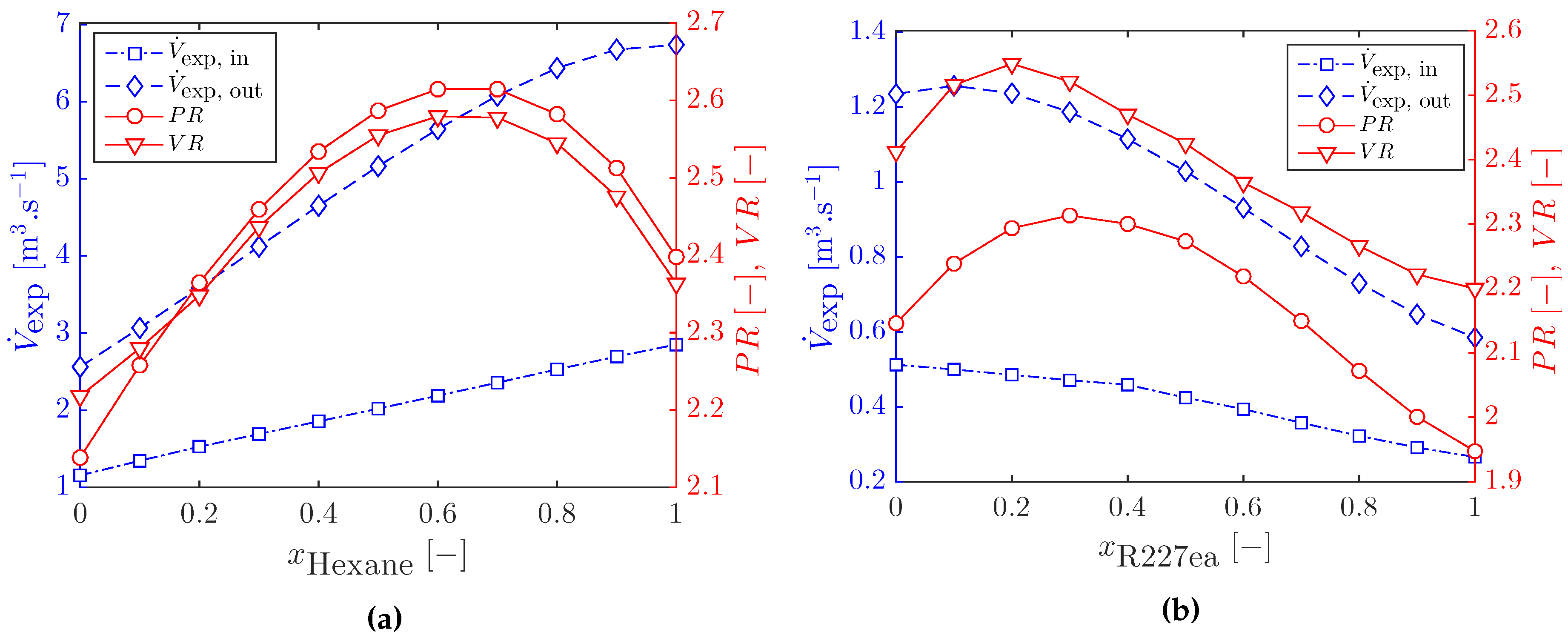
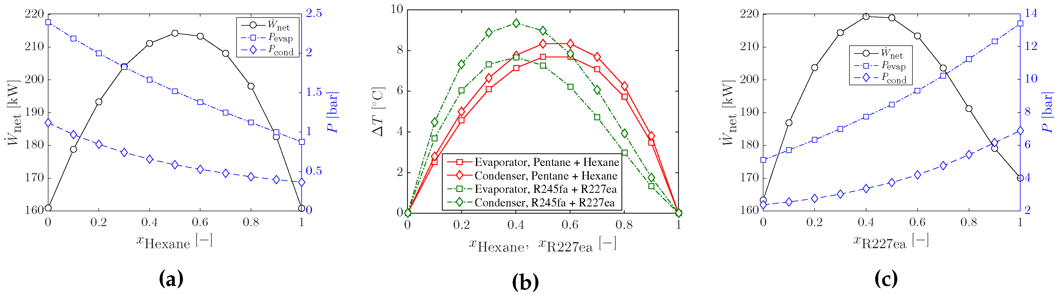
3.1. Optimal Cycles with Working-Fluid Mixtures

The ORC system is optimized for maximum ${\dot{W}}_{\mathrm{net}}$ as described in Equation (13), using the Interior Point algorithm [46]. The optimal power outputs and associated operating pressures are presented in Figure 2, and the expander performance parameters are presented in Figure 3. All other cycle parameters are given in

Table 2. Cycle parameters for ORC systems optimized for maximum net power output using n-pentane + n-hexane and R-245fa + R-227ea working-fluid mixtures.

${\mathit{x}}_{{\mathbf{\text{C}}}_{\mathbf{6}}{\mathbf{\text{H}}}_{\mathbf{14}}}$	${\dot{\mathit{W}}}_{\mathbf{\text{net}}}$	${\mathbf{\eta }}_{\mathbf{\text{th}}}$	${\mathit{w}}_{\mathbf{\text{exp}}}$	${\dot{\mathit{W}}}_{\mathbf{\text{pump}}}$	${\dot{\mathit{m}}}_{\mathbf{\text{wf}}}$	${\mathit{d}}_{\mathbf{\text{SH}}}$	${\dot{\mathit{m}}}_{\mathbf{\text{cs}}}$	${\dot{\mathit{Q}}}_{\mathbf{\text{PH}}}$	${\dot{\mathit{Q}}}_{\mathbf{\text{Ev}}}$	${\dot{\mathit{Q}}}_{\mathbf{\text{DSh}}}$	${\dot{\mathit{Q}}}_{\mathbf{\text{Cn}}}$	${\mathit{x}}_{\mathbf{\text{227ea}}}$	${\dot{\mathit{W}}}_{\mathbf{\text{net}}}$	${\mathbf{\eta }}_{\mathbf{\text{th}}}$	${\mathit{w}}_{\mathbf{\text{exp}}}$	${\dot{\mathit{W}}}_{\mathbf{\text{pump}}}$	${\dot{\mathit{m}}}_{\mathbf{\text{wf}}}$	${\mathit{d}}_{\mathbf{\text{SH}}}$	${\dot{\mathit{m}}}_{\mathbf{\text{cs}}}$	${\dot{\mathit{Q}}}_{\mathbf{\text{PH}}}$	${\dot{\mathit{Q}}}_{\mathbf{\text{Ev}}}$	${\dot{\mathit{Q}}}_{\mathbf{\text{DSh}}}$	${\dot{\mathit{Q}}}_{\mathbf{\text{Cn}}}$
	kW	%	$\mathbf{\text{kJ}}\mathbf{·}{\mathbf{\text{kg}}}^{\mathbf{-}\mathbf{1}}$	kW	$\mathbf{\text{kg}}\mathbf{·}{\mathrm{s}}^{\mathbf{-}\mathbf{1}}$	-	$\mathbf{\text{kg}}\mathbf{·}{\mathrm{s}}^{\mathbf{-}\mathbf{1}}$	MW	MW	MW	MW		kW	%	$\mathbf{\text{kJ}}\mathbf{·}{\mathbf{\text{kg}}}^{\mathbf{-}\mathbf{1}}$	kW	$\mathbf{\text{kg}}\mathbf{·}{\mathrm{s}}^{\mathbf{-}\mathbf{1}}$	-	$\mathbf{\text{kg}}\mathbf{·}{\mathrm{s}}^{\mathbf{-}\mathbf{1}}$	MW	MW	MW	MW
0.0	161	5.00	21.1	2.17	7.74	0.45	73.1	0.47	2.75	0.30	2.75	0.0	163	4.97	11.5	4.05	14.5	1.00	74.7	0.50	2.78	0.48	2.64
0.1	179	5.25	21.8	2.20	8.29	0.18	77.2	0.53	2.88	0.23	3.00	0.1	187	5.17	11.8	5.18	16.2	1.00	82.1	0.60	3.01	0.52	2.92
0.2	193	5.43	22.5	2.16	8.68	0.00	80.5	0.57	2.99	0.18	3.19	0.2	204	5.30	11.7	6.44	18.0	0.84	87.1	0.70	3.15	0.49	3.15
0.3	204	5.55	23.3	2.05	8.86	0.00	83.2	0.59	3.09	0.19	3.29	0.3	214	5.39	11.1	7.88	19.9	0.54	90.1	0.78	3.20	0.41	3.36
0.4	211	5.61	23.7	1.92	8.98	0.00	84.9	0.61	3.15	0.20	3.35	0.4	219	5.42	10.3	9.66	22.3	0.11	91.6	0.87	3.17	0.25	3.58
0.5	214	5.64	23.9	1.78	9.03	0.00	85.8	0.62	3.18	0.20	3.38	0.5	219	5.40	9.79	11.0	23.5	0.12	91.7	0.91	3.14	0.26	3.57
0.6	213	5.61	23.8	1.62	9.02	0.00	85.8	0.62	3.18	0.21	3.38	0.6	213	5.33	9.02	12.7	25.1	0.00	90.6	0.95	3.05	0.21	3.57
0.7	208	5.55	23.4	1.44	8.94	0.00	84.7	0.60	3.15	0.20	3.34	0.7	204	5.21	8.29	14.3	26.3	0.00	88.6	0.97	2.94	0.22	3.48
0.8	198	5.44	22.7	1.26	8.77	0.00	82.4	0.58	3.06	0.20	3.24	0.8	191	5.06	7.52	15.9	27.5	0.00	85.9	0.98	2.81	0.22	3.37
0.9	183	5.28	21.7	1.06	8.48	0.00	78.4	0.53	2.93	0.19	3.09	0.9	179	4.89	6.80	17.9	29.0	0.00	83.3	0.99	2.67	0.23	3.25
1.0	161	5.05	20.2	0.85	8.02	0.00	72.3	0.47	2.71	0.17	2.85	1.0	170	4.76	6.19	20.2	30.7	0.00	81.4	1.02	2.55	0.24	3.17

.

From Table 2, the total rate of heat inflow to the cycle (in all cases) varies between 3.2 MW and 4.0 MW. Of this total, ∼85% is used to evaporate the alkane working fluids (70%−85% for the refrigerants) and the rest is used to pre-heat the fluids to their bubble points. On average, about 3.5 MW is rejected from the cycles, 85% of which is rejected in the condensation process. A working-fluid mixture with $x_{{\mathrm{C}}_6{\mathrm{H}}_{14}}$ = 0.5 results in the cycle with the highest net-power output and thermal efficiency. The (pure) n-hexane cycle has the lowest power output (Figure 2a), followed closely by the n-pentane cycle; their power outputs are about 26% lower than that of the optimal mixture. For the R-245fa + R-227ea system, the mixture with $x_{\mathrm{R-227ea}}$ = 0.4 is the optimal working fluid (Figure 2c).

The working-fluid mixtures with n-hexane fractions between 40% and 60% have the highest specific work-outputs (defined as $w_{\exp }={\dot{W}}_{\exp }/{\dot{m}}_{\mathrm{wf}}$), with $x_{{\mathrm{C}}_6{\mathrm{H}}_{14}}$ = 0.5 having the highest, and the highest working-fluid flow-rates (from Table 2) and therefore also the highest net power-outputs in the considered application. While the pure fluids have the lowest mass flow-rates, they result in cycles with the lowest specific work-outputs due to their lower net-power outputs. Their specific work-outputs are ∼12% lower than that of the optimal fluid-mixture. For the R-245fa + R-227ea system, the optimal working-fluid flow-rate increases monotonically from pure R-245fa to pure R-227ea, and R-227ea has the cycle with the lowest specific work.

As expected, the temperature glides (Figure 2b) are smaller in the evaporator than in the condenser. In both heat exchangers, these follow a parabolic variation with x, reaching a maximum of 7.5 K−8.0 K at $x_{{\mathrm{C}}_6{\mathrm{H}}_{14}}$ = 0.5 (n-pentane + n-hexane) and 7.5 K−9.0 K at $x_{\mathrm{R-227ea}}$ = 0.4 (R-245fa + R-227ea). These directly correspond to the optimal mixtures. In fact, the temperature glide is a reasonably good predictor of the maximum power-output in our study, since high power-output mixtures have relatively high temperature glides, which are also closer to the external heat sink temperature changes (10 ${}^{\circ }$C). Although this holds true for closely related binary mixtures, it has been suggested that mixtures of highly dissimilar fluids may not follow this trend [5,18,34].

From the values of $d_{\mathrm{SH}}$ in Table 2, it is clear that most of the optimal cycles are achieved with zero superheat, $d_{\mathrm{SH}}=0$ (i.e., expanding from a saturated vapour state, without superheating) or minimal superheat. This is because these working fluids are slightly dry in nature (i.e., on the T–s diagram, they have a dew-point curve with a large positive slope) and, as such, superheating is detrimental to cycle performance. Only cycles with mixtures with high proportions of R-245fa are optimized while employing high values of superheat, due to their almost isentropic nature (i.e., almost vertical dew point line on the T–s diagram). On average, the mass flow-rate of the cooling water needed to condense the working fluids is $85\mathrm{kg}·{\mathrm{s}}^{-1}$. It should be noted that the cooling-water flow-rates are over three times larger than the heat-source flow-rate and about ten times larger than the working-fluid flow-rates due to the low temperature change (10 ${}^{\circ }$C) imposed on the cooling stream.

The optimal evaporation and condensation pressures (Figure 2a,c, RHS axes) reduce linearly from n-pentane (R-227ea) to n-hexane (R-245fa). This is because the saturation pressures of n-pentane (R-227ea) are higher than those of n-hexane (R-245fa) at the same temperature, since the critical temperature of n-pentane (R-227ea) is lower than that of n-hexane (R-245fa). In the R-245fa + R-227ea system, the entire condensation process occurs at above atmospheric pressures, whereas in the n-pentane + n-hexane system, only n-pentane condenses at above atmospheric conditions (the other working fluids condense at sub-atmospheric pressures). The pumping power (while being negligible compared to the expander output) mirrors the behaviour of the optimal evaporation pressure in both working-fluid systems.

The volumetric flow-rates through the expander, ${\dot{V}}_{\exp }$ (Figure 3a,b, LHS axes) are linear, increasing steadily from n-pentane (R-227ea) to n-hexane (R-245fa) due to the reduction in the saturation pressures during evaporation and condensation at higher concentrations of n-hexane (R-245fa). The pressure ratio, $PR$, and volumetric expansion ratio, $VR$, (Figure 3a,b, RHS axes) follow similar trends, with a minimum observed for one of the pure-fluid components (n-pentane and R-227ea, respectively), and a maximum observed for a fluid mixture. The low expansion-ratios and volumetric flow-rates for the pure components suggest they would require smaller expanders than the mixtures, potentially leading to cost savings. In addition, they would require fewer expansion stages as volumetric expanders are produced with a fixed ratio, further increasing the potential cost savings.

3.2. Sizing and Costing of Optimal ORC Systems

In the previous section, we demonstrated, for a specific application and choice of fluids, the thermodynamic benefits of employing working-fluid mixtures in ORCs, especially for cases when the heat source and sink profiles are constrained. As expected, there are working-fluid mixtures that realize higher power outputs and efficiencies than both pure fluids as a result of the matching temperature glides during the phase change processes. The associated expansion and pressure ratios of such working-fluid mixtures are comparable to those of the pure working-fluids.

However, these results were derived purely from a thermodynamic perspective; the effects of such mixtures on the heat transfer processes in the heat exchangers, and especially the evaporator and the condenser, have not yet been considered. Experimental investigations have shown that working-fluid mixtures are likely to experience lower HTCs than pure fluids under similar conditions. Thus, it is imperative to examine the consequences of selecting fluid mixtures on the heat transfer processes in an ORC system, with a view towards determining the sizes and costs of the main system components, and therefore their contributions to overall system cost. The pump and expander costs depend on their power ratings and volume/pressure ratios, which were derived from the thermodynamic optimization and thus need no further treatment. The costs of the heat exchangers, on the other hand, depend on their sizes, which cannot be obtained from thermodynamic calculations alone, and require appropriate heat transfer models as presented in Section 2.2.

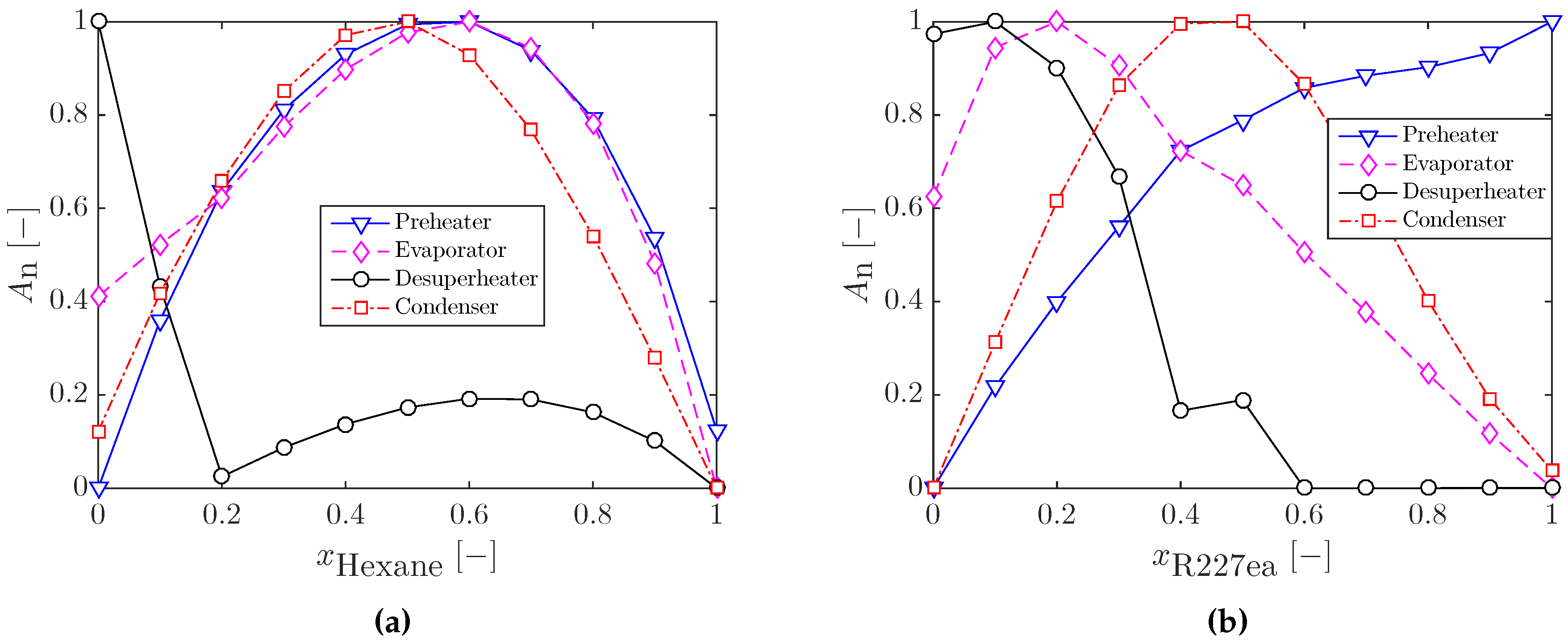
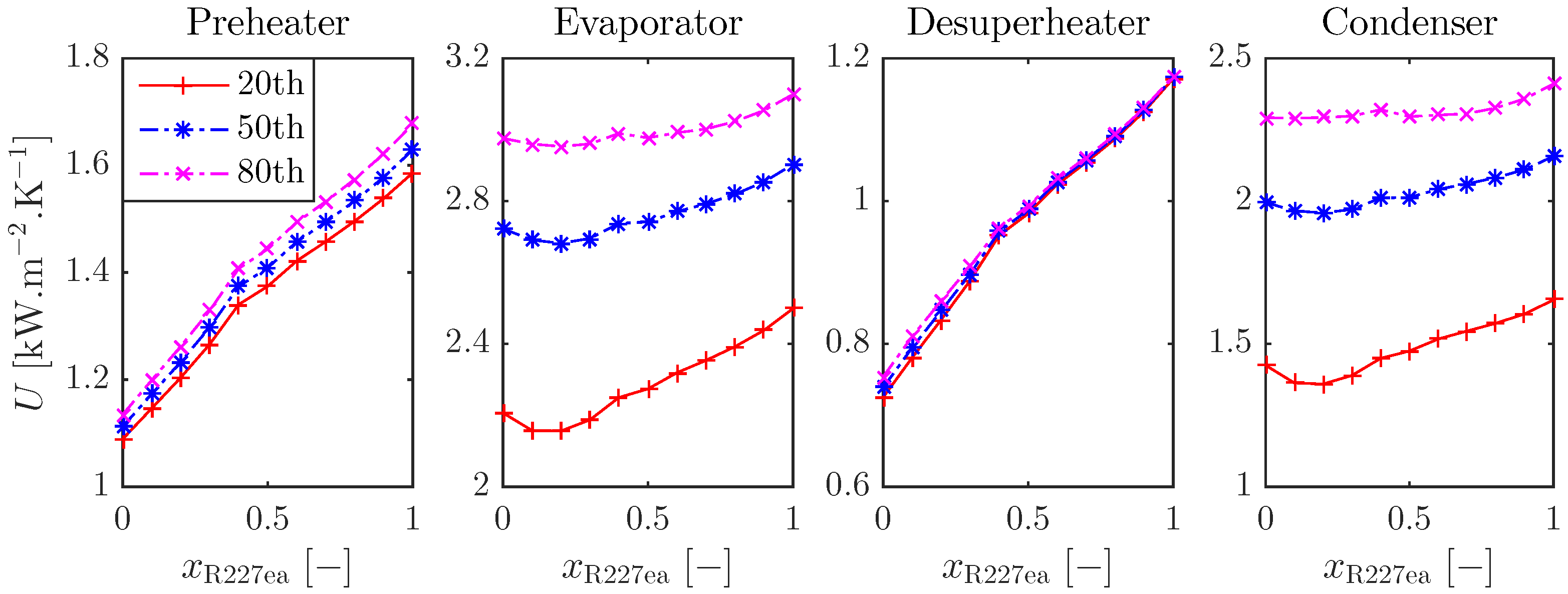
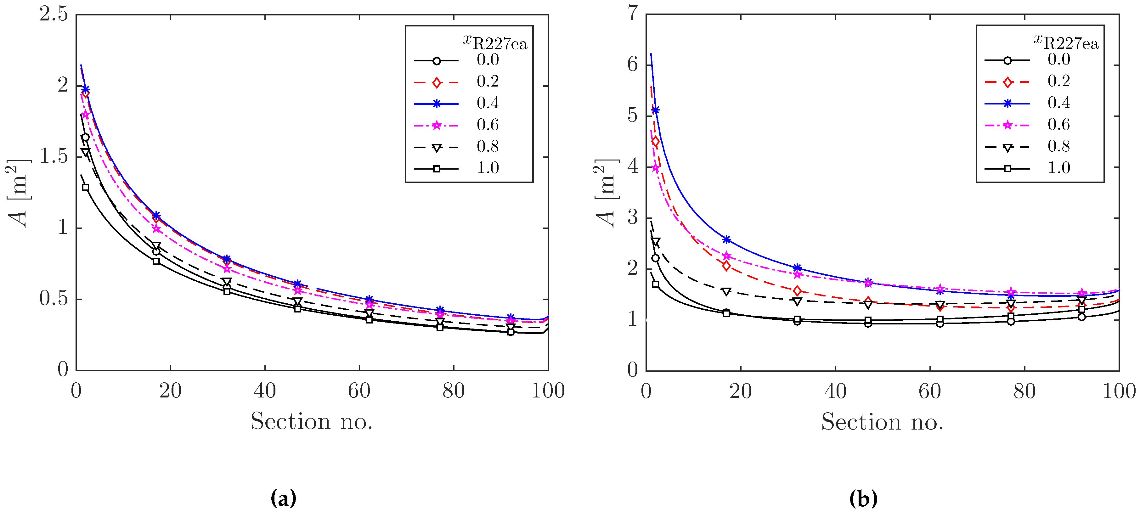
3.2.1. Heat Exchanger Sizing for Optimal ORC Systems

First, we verify the overall heat-transfer coefficients (HTCs) calculated using Equations (9)−(10), especially for the heat exchangers involving phase change (Evaporator and Condenser). The overall HTCs at the 20th, 50th and 80th segments of these heat exchangers, and for the single-phase heat exchangers, are presented in Figure 4 for the R-245fa + R-227ea system. The calculated values are generally in good agreement with experimental data obtained for flow boiling of refrigerant mixtures found in Jung et al. and Shin et al. [23,37]. Also in agreement with experimental observations, the HTCs for the fluid mixtures at each of the segments appear lower than the linearly interpolated values between the two pure-fluid components that make up the mixture. While various explanations have been proposed for this phenomenon, most authors contend that it is due to mass-transfer effects caused by the composition differences between the vapour and liquid phases during the phase-change process.

In the single-phase heat exchangers (Preheater and Desuperheater), the overall HTCs for the mixtures are also lower than the linearly interpolated values, although this deviation is less pronounced for the R-245fa + R-227ea mixtures. Overall, the HTCs are highest in the Evaporator, followed by the Condenser, and lowest in the Desuperheater. Higher HTCs are achieved in the Condenser and Evaporator due to change of phase. The working-fluid vapour results in the low HTC values in the Desuperheater. It should be noted that, in some cases, the Evaporator also serves to superheat the working fluid (for cases where $0\le x_{\mathrm{R-227ea}}\le 0.5$) and, as such, the working fluid exists as a superheated vapour in later segments of the Evaporator. The HTCs in these superheating segments are similar to those exhibited in the Desuperheater in Figure 4. Furthermore, the HTCs presented here are those for the R-245fa + R-227ea system; similar conclusions can be drawn from those of the n-pentane + n-hexane and these are thus omitted.

Based on the knowledge of the HTCs and the associated heat-transfer rates, the heat transfer areas (HTAs) for all segments of the heat exchangers can be calculated from Equation (8). The HTAs of the segments in the Evaporator and the Condenser (for R-245fa + R-227ea) are presented in Figure 5; similar observations can be made by considering n-pentane + n-hexane. As the mole fraction of R-227ea is increased in the mixture, the HTA is seen to increase and then decrease such that the pure fluids (R-245fa and R-227ea) have heat exchangers with the lowest HTAs. This is the case across all of the segments and in both the Evaporator and the Condenser as a direct result of the lower HTCs of the working-fluid mixtures, with the only exception being that of the Evaporator for R-245fa + R-227ea where some mixtures (e.g., $x_{\mathrm{R-227ea}}$ = 0.8) have lower HTAs than pure R-245fa; pure R-227ea still has the lowest areas across all of the sections.

From Figure 5, the HTA variations are less pronounced in the Evaporator than in the Condenser, where large differences exist between the pure fluids and the mixtures. The pure fluids have the smallest heat transfer areas primarily due to their higher HTC values. While the variation in HTA with choice of working fluid (pure and mixtures) across both types of equipment is a result of their varying heat-transfer coefficients, there are larger variations in the Condensers due to the larger heat duties (see Table 2) and larger working-fluid volumetric flow-rates (see Figure 3a,b) handled by the Condensers. Another factor that contributes to this is the large mass flow-rate of cooling water (average of ∼80 kg·s${}^{-1}$ from Table 2) compared to that of the heat source (27 kg·s${}^{-1}$).

The total HTAs for each of the heat exchangers with the different working-fluid mixtures are presented in Figure 6, in normalized form with respect to (based on parameters in

Table 3. Normalization parameters used in Equation (14).

Pentane + Hexane	PH	Ev	DSh	Cn	R-245fa + R227ea	PH	Ev	DSh	Cn
$A_{\min }$ (m${}^2$)	21.8	48.5	15.8	80.8	$A_{\min }$ (m${}^2$)	24.5	51.1	15.2	109
$A_{\max }$ (m${}^2$)	25.8	65.3	23.4	150	$A_{\max }$ (m${}^2$)	37.2	82.6	29.9	204

):

$$A_{\mathrm{n}}=(A_{\mathrm{HX}}-A_{\min })/(A_{\max }-A_{\min }).$$

(14)

The absolute total heat-transfer area gives a direct indication of the size of the heat exchanger, while the normalized form facilitates the comparison between the different fluid mixtures. As expected by considering their thermal duties (see Table 2), the Evaporators are generally 2−3 × larger than the Preheaters, while the Condensers are 5−6× larger than the Desuperheaters. Although the Condenser thermal-duties are only about 15% higher than those of the Evaporators, the Condensers are twice (or more) as large as the Evaporators in most instances. This is due to the lower overall HTCs and the lower temperature differences across the Condensers. This is further magnified by the lower pressures in the Condensers (compared to the Evaporators), leading to higher working-fluid volumetric flow-rates (${\dot{V}}_{\mathrm{exp,out}}>{\dot{V}}_{\mathrm{exp,in}}$, see Figure 3) and, hence, much larger Condenser sizes.

From the thermodynamic optimization results in Table 2, it can be seen that although most of the optimal cycles are achieved without superheating ($d_{\mathrm{SH}}=0$), a few ($x_{{\mathrm{C}}_6{\mathrm{H}}_{14}}$ = 0, 0.1, and $x_{\mathrm{R-227ea}}\le 0.5$) do however involve varying degrees of superheat ($d_{\mathrm{SH}}>0$), and thus would require a superheating section to be added to their Evaporators. The effect of this addition, is that these systems (with high degrees of superheat) will require larger Evaporators as is noticeable for both sets of working-fluid mixtures in Figure 6. For the n-pentane + n-hexane mixtures, ORC systems with $x_{{\mathrm{C}}_6{\mathrm{H}}_{14}}$ = 0 or $x_{{\mathrm{C}}_6{\mathrm{H}}_{14}}$ = 0.1 do not follow the general parabolic trend established with the other working-fluid mixtures. Their Evaporator HTAs are seen to be larger than expected from the trend due to this additional superheating section. This effect is even more pronounced for the R-245fa + R-227ea mixtures, which exhibit optimal cycles with larger degrees of superheat. The Evaporator HTAs for ORC systems with $0.1\le d_{\mathrm{SH}}\le 1$ (i.e., those with $x_{\mathrm{R-227ea}}\le 0.5$) are much larger than those with $x_{\mathrm{R-227ea}}>0.5$ that do not require a superheating section.

Furthermore, in systems that require an additional superheating section, the working-fluid vapour exits the evaporator and, therefore, enters the expander at higher temperatures, and subsequently it exits the expander with higher degrees of superheat and at higher temperatures. This requires a larger amount of heat to be rejected to the cooling stream in the desuperheater, as a consequence of which these systems (with $d_{\mathrm{SH}}>0$) typically require larger desuperheaters than the systems with $d_{\mathrm{SH}}=0$. This inference can be seen in Figure 6 for both the n-pentane + n-hexane and R-245fa + R-227ea working-fluid systems, accounting for the two regimes in the normalized desuperheater HTA in both systems. The ORC systems with $d_{\mathrm{SH}}>0$ (i.e., $0\le x_{{\mathrm{C}}_6{\mathrm{H}}_{14}}<0.2$ and $0\le x_{\mathrm{R-227ea}}<0.5$, see Table 2) have larger normalized DSh areas than those with $d_{\mathrm{SH}}=0$. Thus, superheating the working fluid in ORC evaporators not only increases the size (HTA) of the Evaporator but also the size of the Desuperheater and eventually the cost of the engine as a whole.

As the concentration of R-227ea in the refrigerant-mixture system is increased, the PH heat duties increase, and so does its total HTA. The PH areas for the n-pentane + n-hexane systems are also directly governed by their heat duties. It should, however, be noted that these variations in HTA with working-fluid mixtures (maximum range of 13 m² and 15 m² for the preheaters and desuperheaters, respectively) are much smaller than those associated with the two-phase heat exchangers (maximum range of 32 m² and 95 m² for the evaporators and condensers respectively). This is important, in that it suggests that working-fluid mixtures have a more profound effect on the Evaporator and Condenser sizes than they do on the single-phase heat-exchangers, at least in the present study.

From Figure 6, it is clear that the pure working-fluids have smaller Evaporator HTAs compared to the mixtures. The only minor exception is found in the R-245fa + R-227ea system, where fluid mixtures with $x_{\mathrm{R-227ea}}\ge 0.9$ have lower Ev areas than pure R-245fa. Furthermore, due to the deterioration of HTCs during condensation, the Condensers for the working-fluid mixtures are much larger than those for the pure fluids. In the case of the R-245fa + R-227ea system, the Condenser HTAs range from 109 m² ($x_{\mathrm{R-227ea}}$ = 0) to 204 m² ($x_{\mathrm{R-227ea}}$ = 0.5). This implies an increase in HTA of 85% when a working-fluid mixture is substituted for a pure working fluid (or, conversely, a decrease in HTA of 45% when a working-fluid mixture is substituted with a pure working fluid). Such large differences in HTAs between working-fluid mixtures and pure fluids can lead to considerable differences in plant size and cost, in favour of the pure working fluids.

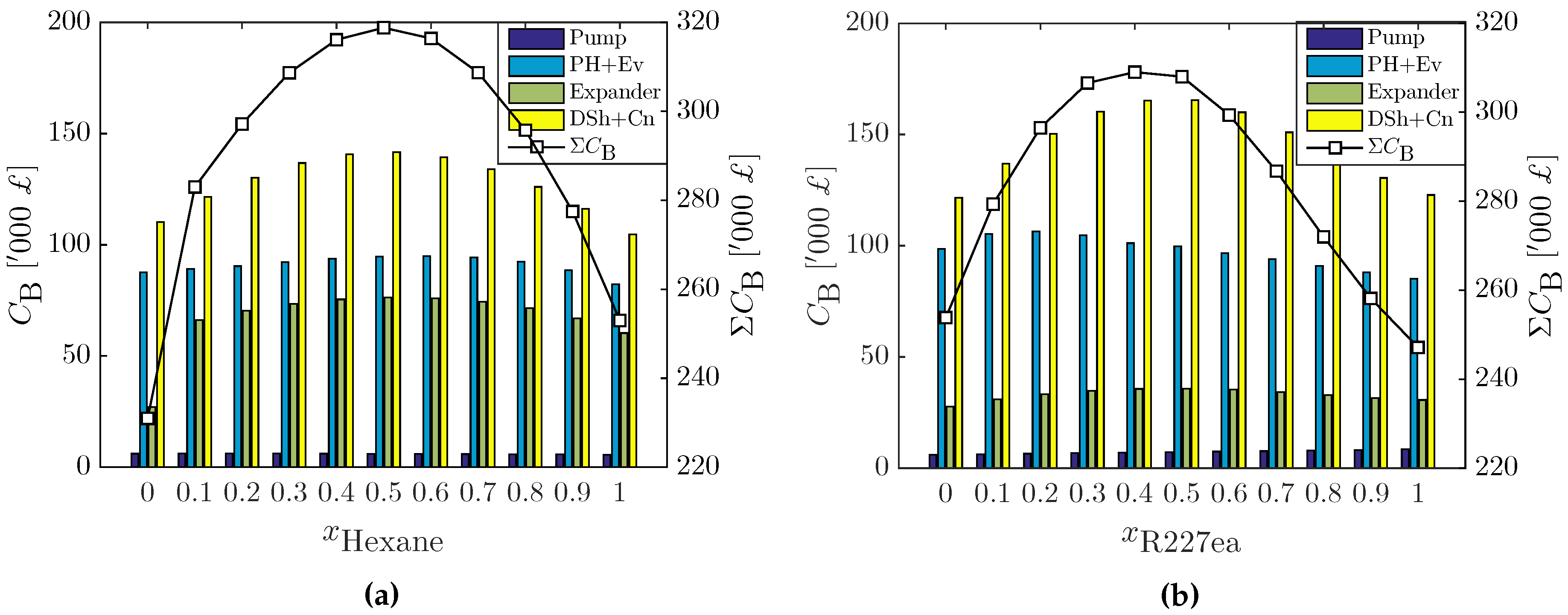
3.2.2. Cost Estimation of Optimal ORC Systems

With the heat transfer areas of the heat exchangers determined, all the equipment size factors required in Table 1 for the estimation of the ORC component costs are now defined. With these size factors, we now proceed to evaluate the costs of the ORC components. The calculated component-base costs of the optimal ORC systems are presented in Figure 7 (LHS axes).

The pumps (combined with their motors) cost around £6,000, with the cost reducing monotonically from pure n-pentane (R-227ea) to n-hexane (R-245fa) as a direct result of the lower evaporation pressures as the concentration of n-hexane (R-245fa) in the working fluid is increased (in line with Figure 2). Similarly, the costs of the single-phase heat exchangers (PH and DSh) are low (£9,000−£10,000). However, the evaporator and condenser costs are well in excess of £80,000. The expander costs fall into two classes: (i) sub-atmospheric pressure (vacuum) discharge expanders that cost between £65,000−£75,000; and (ii) standard expanders with a considerably lower cost between £25,000−£35,000. From these results, it is clear that the expander and the phase-change heat exchangers present the dominant costs of the ORC system considered here.

The pure fluids (pure n-pentane and n-hexane; R-245fa and R-227ea) generally have the lowest-cost evaporators and condensers, while the mixtures ($x_{{\mathrm{C}}_6{\mathrm{H}}_{14}}$ = 0.6 and $x_{{\mathrm{C}}_6{\mathrm{H}}_{14}}$ = 0.5; $x_{\mathrm{R-227ea}}$ = 0.2 and $x_{\mathrm{R-227ea}}$ = 0.5, respectively) have the highest costs. This is a direct result of the pure working fluids having higher heat-transfer coefficients (due to the deterioration of heat transfer behaviour of the mixtures) than the working-fluid mixtures and thus their lower heat transfer areas and subsequent lower costs. In addition, the higher power output produced by the mixtures is achieved partly by their high heat duties (see Table 2), contributing to their larger HTAs and heat exchanger costs and resulting in cheaper heat exchangers for the ORC systems with pure working fluids.

From Figure 7a,b, it is clear that the expander costs mirror the trend exhibited by the optimal power output in Figure 2a,c especially as they are correlated with the power output. However, for the n-pentane + n-hexane system, the expander cost for pure n-pentane ($x_{{\mathrm{C}}_6{\mathrm{H}}_{14}}$ = 0) is over 50% lower than those of the other working fluids. After expansion, the n-pentane vapour exits the expander at above atmospheric pressure while all the other working fluids exit at sub-atmospheric pressures (i.e., below 1 atm) and had their expander costs calculated with the low-pressure discharge expander correlation in Table 1. This, in turn, makes the cost of the n-pentane expander much lower than the rest in the n-pentane + n-hexane system. On the other hand, all the working fluids in the R-245fa + R-227ea system exit the expander above atmospheric pressure; this makes the expanders and the ORC engines (total cost on RHS axes of Figure 7) of the R-245fa + R-227ea system cheaper than those of the n-pentane + n-hexane system.

It should be noted that the cost figures presented in this work (here in Figure 7, and subsequently in Figure 8, Figure 9, Figure 10 and Figure 11) are preliminary, simple estimations based on the specific costing exercise presented in Section 2.3, and therefore subject to the assumptions and accuracy of this exercise. It is inevitable that the final cost values are more difficult to quantify rigorously, and are associated with uncertainties that are larger than those in the thermodynamic analysis. Specifically, the cost figures can be expected to vary by about ±25% as stated in Section 2.3, and the actual capital costs of the associated plants can be different from those presented by a similar margin. Furthermore, employing any of the other cost correlations mentioned in Section 2.3 would result in new cost figures, different in magnitude from those in this work. Nevertheless, the qualitative (relative) comparisons derived from these figures (Figure 7, Figure 8, Figure 9, Figure 10 and Figure 11), with regards to the effect of the choice of working fluid (i.e., pure or working-fluid mixtures) are less sensitive to the absolute cost figures and should remain as presented herein. This is to be expected since the component cost calculations were based on the physical sizes of the equipment and these (the equipment sizes) are directly affected by the choice of working fluid.

The total base cost for the ORC systems is presented on the RHS axes in Figure 7. By comparing the individual component-base costs to the total cost, one can arrive at a component cost distribution for typical ORC systems. The pumps generally have the lowest proportion of the total cost, usually less than 3% while the expander (depending on the type) can contribute between 10% and 25% to the total cost. Due to their special construction, vacuum discharge expanders are more expensive than standard ones and thus they can contribute up to 25% of the total cost. The heat addition heat exchangers (Preheater and Evaporator) make up about 35% of the total costs, while the heat rejection heat exchangers (Desuperheater and Condenser) make up between 45% and 55% of the total cost. This implies that the heat exchangers can make up to 90% of the combined component cost of ORC systems, highlighting the consequence of employing (or not) working-fluid mixtures on the overall ORC plant cost and the need to investigate the compromise between the thermodynamic benefits and the cost implications of more working-fluid mixture systems.

3.3. Heat Input Limitations and Other Working-Fluid Mixtures

While we have demonstrated the benefits and drawbacks of working-fluid mixtures in ORCs with two pairs of fluids (n-pentane + n-hexane and R-245fa + R-227ea), it is important to investigate other working fluid systems of practical interest. Along with the four initial pure fluids, we also consider mixtures of the following alkanes and refrigerants: n-butane, R-134a, R-236fa and R-245ca. Although this list is not an exhaustive selection of the huge number of mixture combinations possible, it will give some indication of the behaviour of mixtures with ORCs in general. In addition, we investigate alternative ORC system designs in which the heat input to the cycle is fixed as may be practically required, e.g., due to retrofits or a need of the heat source for other purposes such as heating or otherwise; this further presents another basis of comparison of pure working fluids and working-fluid mixtures in ORCs. This is done by limiting the heat extracted from the heat source such that ${\dot{Q}}_{\mathrm{in}}\le {\dot{Q}}_{\mathrm{in,lim}}$. Three cases are provided:

• ${\dot{Q}}_{\mathrm{in,lim}}$ is allowed to attain a maximum possible value; this is the case in Section 3.1 where the optimal cycle heat input (${\dot{Q}}_{\mathrm{in}}$) for different working fluids is seen to vary between 3.2 MW and 4.0 MW.
• ${\dot{Q}}_{\mathrm{in,lim}}=2.5$ MW.
• ${\dot{Q}}_{\mathrm{in,lim}}=1.0$ MW.

In all the cases, the cycles are optimized to maximize the net power output, subject to the heat exchangers’ pinch conditions. Cases 2 and 3 are further limited by the heat input constraints (${\dot{Q}}_{\mathrm{in}}\le {\dot{Q}}_{\mathrm{in,lim}}$), corresponding to heat source outlet temperatures of 76.0 ${}^{\circ }$C and 89.2 ${}^{\circ }$C, respectively. In particular, the case of 1.0 MW heat input is replicative of the conditions in the original plant. The maximum net power output for the three cases, using different working fluid mixtures are presented in Figure 8, Figure 9 and Figure 10, respectively. Here also, the component costs of the optimal ORC systems are reported in terms of their ‘rated costs’, i.e., cost per kilowatt of net power generated ($\Sigma C_{\mathrm{B}}$/${\dot{W}}_{\mathrm{net}}$). This is done such that high power output fluids (especially the fluid mixtures which will have higher total costs) are not unnecessarily penalized.

The working-fluid mixtures are seen to produce higher power outputs than the pure fluids in all three cases. In Case 1 (${\dot{Q}}_{\mathrm{in,lim}}$ is allowed to attain a maximum possible value), the fluid mixtures generally lead to systems with lower rated costs (in pounds per kW) than the pure fluids with only a few exceptions (R-245ca + R-245fa where R-245ca has the least cost and R-236fa + R-245fa where R-245fa has the least cost). This is due to the higher net power derived from cycles with mixtures over those with pure fluids, keeping their rated costs lower (although the have higher total costs as in Figure 7). It should, however, be noted that the objective here was to maximize the net power output from the cycle. Thus, the cycles with working-fluid mixtures, with their much higher power output, will be expected to lower rated costs in comparison with the pure working fluids. In Section 3.4, we consider a multi-objective cost-power optimization.

For Cases 2 and 3 (Figure 9 and Figure 10), the working-fluid mixtures still result in cycles with the highest power output, but these systems are, however, more expensive (both in terms of the total costs in pounds and the rated costs in pounds per kW) than those with the pure working fluids. A clear exception to these trends is the n-butane + n-hexane working-fluid system, where the working-fluid mixtures are seen to provide lower net power outputs than than the constituent pure fluids. Due to the lower isobaric specific heat-capacities of the mixtures compared to the pure fluids, they are expected to result in lower power output [16]. Their lower net power output is made more pronounced as they also have lower optimal mass flow-rates than the constituent pure working fluids. These invariably translate to the much higher rated costs for ORC systems with n-butane + n-hexane working fluids than those with other working-fluid systems. For most of the fluid pairings, the mixture with the highest net power output usually leads to the most expensive ORC system, while the systems with the pure fluids are usually the cheapest. Here, the gain in power output achieved by the mixtures is not sufficient to overcome the additional cost incurred in the use of larger expanders and heat exchangers due to their poor heat transfer performance.

As a specific example (for Case 3, ${\dot{Q}}_{\mathrm{in,lim}}=1.0$ MW) in the n-pentane + n-hexane system, the ORC system with n-pentane as the working fluid has the lowest rated cost (£2,300 per kW) due to its very low expander cost compared to the other working fluids, while the system with $x_{{\mathrm{C}}_6{\mathrm{H}}_{14}}$ = 0.5 has the highest rated cost at £2,700 per kW. For the R-245fa + R-227ea system, the ORC system with pure R-245fa has the lowest rated cost (about £2,500 per kW) while that with $x_{\mathrm{R-227ea}}$ = 0.5 has the highest rated cost. The thermodynamically optimal fluid mixtures ($x_{{\mathrm{C}}_6{\mathrm{H}}_{14}}$ = 0.4 and $x_{\mathrm{R-227ea}}$ = 0.3) have ORC system rated costs of £2,700 per kW and £2,900 per kW, respectively. On the other hand, the cost optimal working fluids are n-pentane and R-245fa, which give rated cost reductions of 14.8% and 13.8%, respectively, over the thermodynamically optimal working fluids.

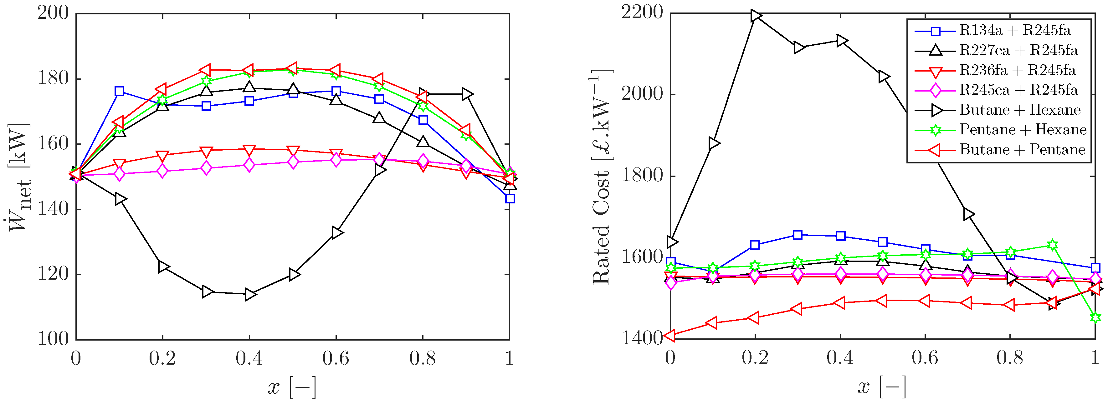
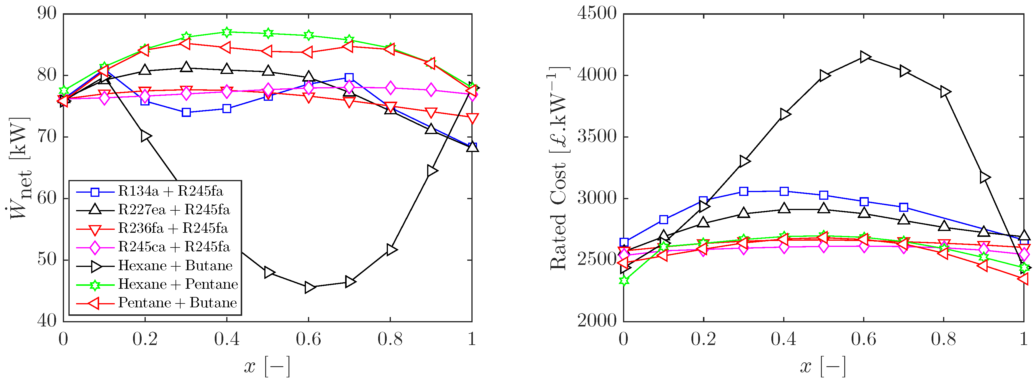
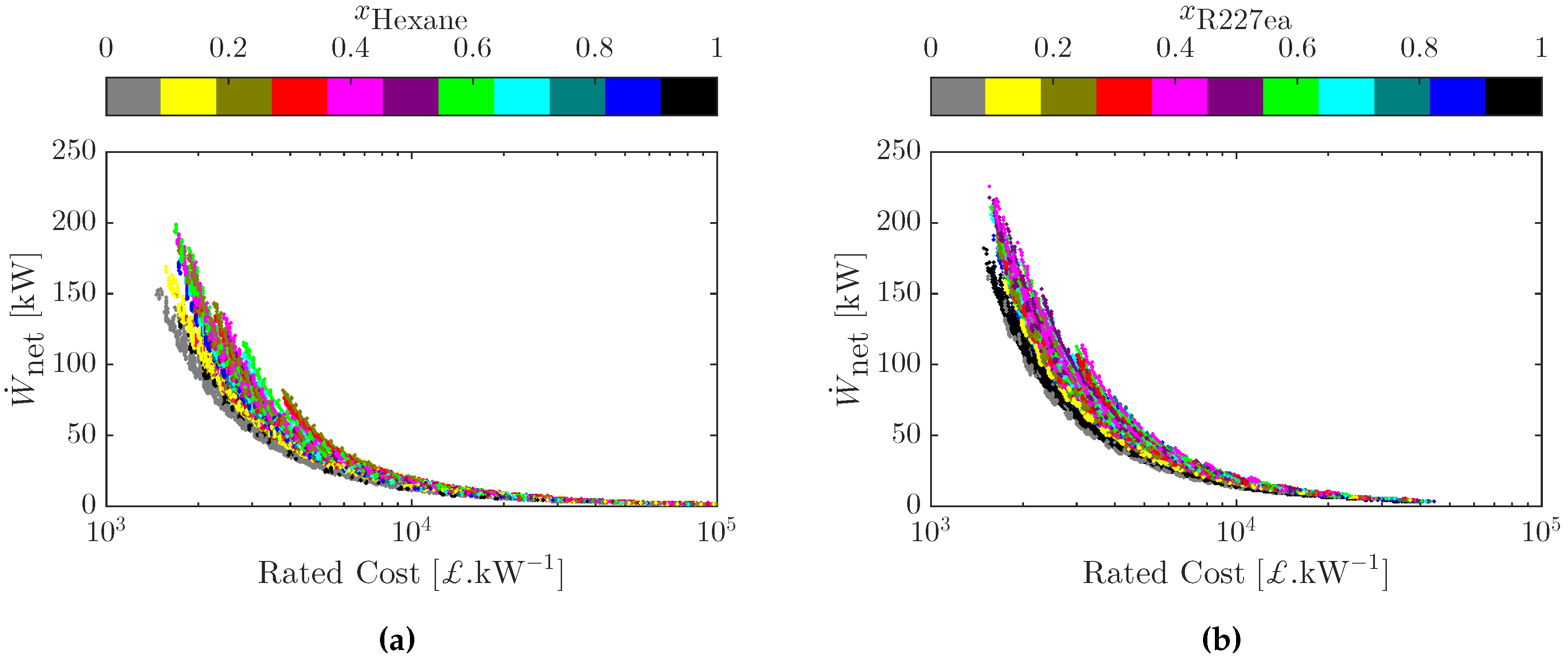
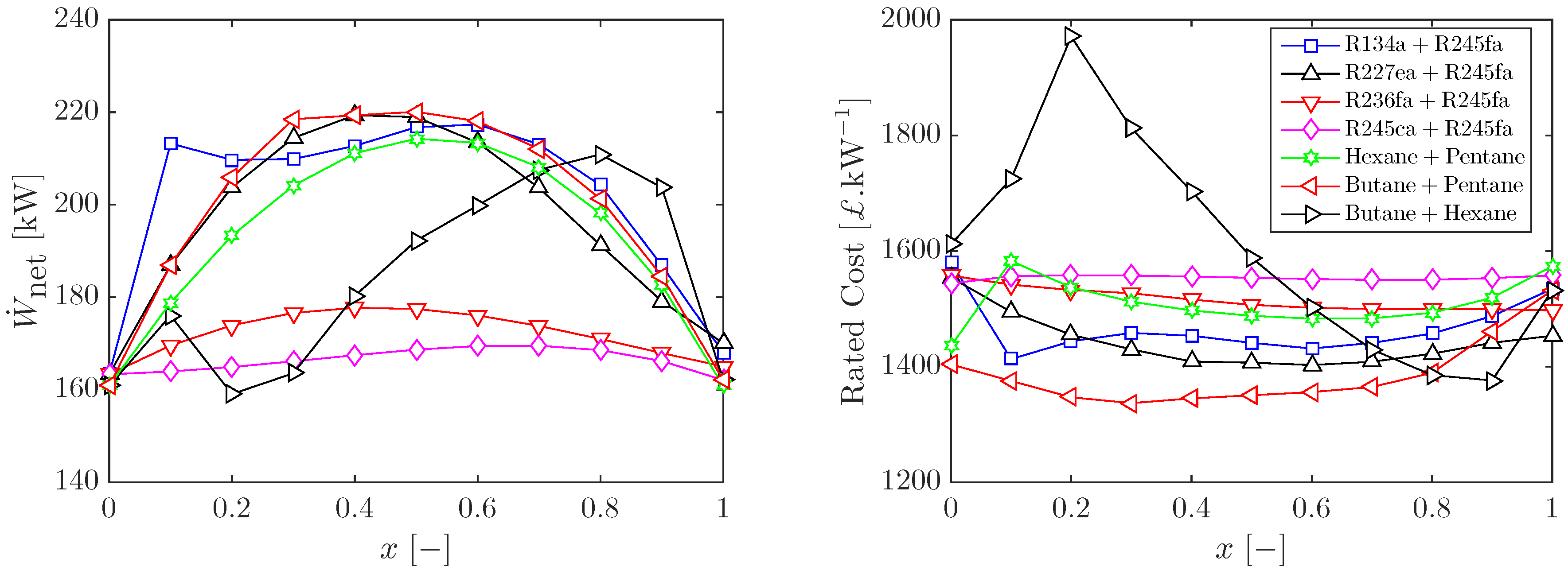
3.4. Multi-Objective Cost-Power Optimization

So far, we have considered the costs of optimal ORC systems in the sense of maximizing the net power output. We conclude this paper with a brief investigation of the simultaneous cost and performance optimization of these systems with pure fluids and working-fluid mixtures. This is carried out in a similar manner to the problem in Equation (13), with no restriction on the heat input into the cycles. The only addition here is change in the objective function to a multi-objective optimization of the net power output (maximization) from the cycles and the rated costs (minimization) of the ORC systems; the constraints remain as earlier stated. The results are presented in Figure 11 for the n-pentane + n-hexane and the R-245fa + R-227ea systems, in form of the pareto optimal curves.

The pareto curves reveal that the two objectives (maximizing the cycles’ net power output and minimizing their systems’ rated costs in pounds per kW) are fairly complementary functions; the cycles with the maximum net power output are the ones that have ORC systems with the minimum rated costs. Ordinarily, the net power output and the total component-base costs (in £) will be competing functions such that ORC systems that maximize the power output will be expensive while the cheap systems (i.e., those with minimum costs) will produce minimal power. This highlights the importance of normalizing the total component-base costs with the cycle net power to derive the rated ORC system costs, thereby making both objectives complimentary. This also reveals the economies of scale in the design of ORC plants; plants with higher power outputs will cost less (in pounds per kW) than those with lower power output—in this instance, ORC systems with net power below 50 kW cost in excess of £5000 per kW while those with power above 150 kW cost below £2000 per kW.

Thus, with reference to the plots in Figure 11, the ORC systems that simultaneously maximize the net power output and minimize the rated costs are those located towards the top-left corner of the plots. Furthermore, the pareto curves are colour coded to distinguish the mixture compositions of the various working-fluid mixtures and pure fluids used in the cycles. From both subplots in Figure 11, one can observe that the working-fluid mixtures always result in cycles with the maximum net power. This directly replicates and reinforces the conclusions from Section 3.1. These ORC systems are, however, not the ones with the least rated costs; the systems with the pure working fluids are the ones that minimize the rated costs.

At the net power levels where systems with pure working fluids are feasible, they are much cheaper than the systems with working-fluid mixtures. For example, in the case of the n-pentane + n-hexane system, at a net power output of 100 kW, systems with pure n-pentane and/or systems with pure n-hexane as working fluid cost below £2000 per kW while those with the working-fluid mixtures can cost up to £3000 per kW, representing a 50% increase in rated cost in using working fluid mixtures. Similarly, in the R-245fa + R-227ea system, ORC systems with the pure working fluids (R-245fa or R-227ea) are generally cheaper than those with the fluid mixtures. These illustrate that, while the working-fluid mixtures may deliver plants with higher power ratings, they do so with considerable additional cost incurred. The pure working fluids on the other hand will produce slightly less power but with the advantage of smaller sized process units and at considerably lower costs.

Previous research efforts into the deployment of working-fluid mixtures (multi-component working fluids) in ORC systems [2,3,4,5,7,8,9,11,12,13,15,18,34,43] have generally considered the thermodynamic benefits of such mixtures in comparison with pure (single component) working fluids, and as exemplified earlier with the results in Section 3.1, the mixtures do give better performance (in terms of net power output and/or thermal/exergy efficiencies) than the pure fluids. These mixtures have, however, been shown to suffer a deterioration in their heat transfer performance especially during the phase-change processes. The overarching consequences of these on the size and costs of ORC systems with such mixtures are yet to be fully explored. The results in this paper are an attempt to quantify and qualify these consequences, in comparison with ORC systems employing pure working fluids.

Recently, Andreasen et al. [47,48] concluded that a 500 kW ORC system with the R32 + R134a working-fluid mixture is cheaper than that with pure R32 as working fluid. However, Heberle and Brüggemann [49,50] showed that ORC systems with pure i-butane as working fluid has a lower specific cost (in €·kW${}^{-1}$) than those with the i-butane + i-pentane working-fluid mixtures. Similarly, ORC systems with pure n-pentane or pure R-227ea were found to be cheaper than those with mixtures of n-pentane + n-hexane or R-245fa + R-227ea, respectively [51]. It should be noted the ORC systems in Ref. [50,51] have lower ratings of about 300 kW and 100 kW, respectively; thus, it can be argued that ORC systems with mixtures may become more cost effective at higher plant ratings. In this paper, we have investigated a more expansive set of working-fluid mixtures across varying ORC plant sizes, and in line with these recent findings [50,51], we can summarize that working-fluid mixtures, although attaining a better thermodynamic performance in ORC systems, lead to larger and more expensive systems. Thus, the ORC systems with pure working fluids are more cost effective.

4. Conclusions

The first aim of this study was to investigate the thermodynamic benefits of employing working-fluid mixtures in organic Rankine cycle (ORC) systems, with a specific focus on an application involving a low-temperature geothermal hot-water heat-source stream; a second aim was to examine the effects of selecting such mixtures on the sizes and costs of the resulting ORC engines. Initially, two sets of fluid mixtures, namely n-pentane + n-hexane and R-245fa + R-227ea, were used for this investigation due to their common use in ORC installations; five other pairs of mixtures were later investigated, as well as ORC systems of different sizes. The thermodynamic optimization (maximum net power output) resulted in optimal working-fluid mixtures in both cases; the performance indices of these mixtures along with corresponding costs are summarized and compared with those of their constituent pure components in Section 3.

The analyses revealed that the temperature glides of the working-fluid mixtures during evaporation and condensation resulted in higher power output and thermal efficiencies for fluid mixtures. Mixtures containing 50% of n-hexane and those with 40% R-227ea had the highest net-power output, delivering up to 30% more power than either set of pure fluids. The pure fluids did however result in smaller expanders due to their low volumetric flow-rates and expansion ratios. Due to their poor phase-change heat transfer characteristics, ORC systems with fluid mixtures appeared to have the largest evaporators and condensers (with their condenser areas up to 80% higher than those of the pure fluids), requiring more expensive heat exchangers than the pure fluids. Moreover, due to sub-atmospheric (vacuum) expansion, the expander costs in the case of the n-pentane + n-hexane working-fluid mixtures (and n-hexane) were much higher than those for pure n-pentane. Generally, and in consonance with recent efforts from other investigators, equipment sizes and costs were larger for both sets of mixtures than for the constituent pure fluids. Thus, the working-fluid mixtures would require larger plant layout areas, contributing significantly to their overall installation costs.

Although the mixtures were found to have the highest power output, they also had the highest rated cost (equipment cost per net kilowatt power generated). On the other hand, a multi-objective cost-power optimization revealed that ORC systems with pure n-pentane working fluid had the lowest rated cost followed by those with n-hexane. For the case of R-245fa + R-227ea working fluids, the ORC system with pure R-227ea had the lowest rated costs, about 14% less than the system with 40% R-227ea working fluid. These observations imply that the thermodynamic benefits derived from using the working-fluid mixtures may be outweighed by the increased costs incurred. The fact that these insights were only possible from a direct consideration of thermal and cost factors, as exemplified here, underlines the importance of employing a combined thermodynamic, thermal and cost approach in the selection of optimal working-fluid (mixtures) for ORC systems.

References

1. Markides, C.N. Low-concentration solar-power systems based on organic Rankine cycles for distributed-scale applications: Overview and further developments. Front. Energy Res. 2015, 3:47, 1–16. [Google Scholar] [CrossRef]
2. Angelino, G.; di Paliano, P.C. Multicomponent working fluids for ORCs. Energy 1998, 23, 449–463. [Google Scholar] [CrossRef]
3. Garg, P.; Kumar, P.; Srinivasan, K.; Dutta, P. Evaluation of isopentane, R-245fa and their mixtures as working fluids for organic Rankine cycles. Appl. Ther. Eng. 2013, 51, 292–300. [Google Scholar] [CrossRef]
4. Wang, J.L.; Zhao, L.; Wang, X.D. A comparative study of pure and zeotropic mixtures in low-temperature solar Rankine cycle. Appl. Energy 2010, 87, 3366–3373. [Google Scholar] [CrossRef]
5. Oyewunmi, O.A.; Taleb, A.I.; Haslam, A.J.; Markides, C.N. On the use of SAFT-VR Mie for assessing large-glide fluorocarbon working-fluid mixtures in organic Rankine cycles. Appl. Energy 2016, 163, 263–282. [Google Scholar] [CrossRef]
6. Lecompte, S.; Lemmens, S.; Huisseune, H.; van den Broek, M.; De Paepe, M. Multi-objective thermo-economic optimization strategy for ORCs applied to subcritical and transcritical cycles for waste heat recovery. Energies 2015, 8, 2714–2741. [Google Scholar] [CrossRef] [Green Version]
7. Sami, S.M. Energy and exergy analysis of new refrigerant mixtures in an organic Rankine cycle for low temperature power generation. Int. J. Ambient Energy 2010, 31, 23–32. [Google Scholar] [CrossRef]
8. Chen, H.; Goswami, D.Y.; Rahman, M.M.; Stefanakos, E.K. A supercritical Rankine cycle using zeotropic mixture working fluids for the conversion of low-grade heat into power. Energy 2011, 36, 549–555. [Google Scholar] [CrossRef]
9. Aghahosseini, S.; Dincer, I. Comparative performance analysis of low-temperature organic Rankine cycle (ORC) using pure and zeotropic working fluids. Appl. Ther. Eng. 2013, 54, 35–42. [Google Scholar] [CrossRef]
10. Gao, H.; Liu, C.; He, C.; Xu, X.; Wu, S.; Li, Y. Performance analysis and working fluid selection of a supercritical organic Rankine cycle for low grade waste heat recovery. Energies 2012, 5, 3233–3247. [Google Scholar] [CrossRef]
11. Heberle, F.; Preißinger, M.; Brüggemann, D. Zeotropic mixtures as working fluids in organic Rankine cycles for low-enthalpy geothermal resources. Renew. Energy 2012, 37, 364–370. [Google Scholar] [CrossRef]
12. Shu, G.; Gao, Y.; Tian, H.; Wei, H.; Liang, X. Study of mixtures based on hydrocarbons used in ORC (organic Rankine cycle) for engine waste heat recovery. Energy 2014, 74, 428–438. [Google Scholar] [CrossRef]
13. Dong, B.; Xu, G.; Cai, Y.; Li, H. Analysis of zeotropic mixtures used in high-temperature organic Rankine cycle. Energy Convers. Manag. 2014, 84, 253–260. [Google Scholar] [CrossRef]
14. Preißinger, M.; Brüggemann, D. Thermal stability of hexamethyldisiloxane (MM) for high-temperature organic Rankine cycle (ORC). Energies 2016, 9, 183. [Google Scholar] [CrossRef]
15. Lecompte, S.; Ameel, B.; Ziviani, D.; van den Broek, M.; De Paepe, M. Exergy analysis of zeotropic mixtures as working fluids in organic Rankine cycles. Energy Convers. Manag. 2014, 85, 727–739. [Google Scholar] [CrossRef]
16. Stijepovic, M.Z.; Linke, P.; Papadopoulos, A.I.; Grujic, A.S. On the role of working fluid properties in organic Rankine cycle performance. Appl. Ther. Eng. 2012, 36, 406–413. [Google Scholar] [CrossRef]
17. Mathkor, R.Z.; Agnew, B.; Al-Weshahi, M.A.; Latrsh, F. Exergetic analysis of an integrated tri-generation organic Rankine cycle. Energies 2015, 8, 8835–8856. [Google Scholar] [CrossRef]
18. Li, Y.R.; Du, M.T.; Wu, C.M.; Wu, S.Y.; Liu, C. Potential of organic Rankine cycle using zeotropic mixtures as working fluids for waste heat recovery. Energy 2014, 77, 509–519. [Google Scholar] [CrossRef]
19. Papadopoulos, A.I.; Stijepovic, M.; Linke, P. On the systematic design and selection of optimal working fluids for organic Rankine cycles. Appl. Ther. Eng. 2010, 30, 760–769. [Google Scholar] [CrossRef]
20. Lampe, M.; Kirmse, C.; Sauer, E.; Stavrou, M.; Gross, J.; Bardow, A. Computer-aided molecular design of ORC working fluids using PC-SAFT. Comput. Aided Chem. Eng. 2014, 34, 357–362. [Google Scholar]
21. Papadopoulos, A.I.; Stijepovic, M.; Linke, P.; Seferlis, P.; Voutetakis, S. Toward optimum working fluid mixtures for organic Rankine cycles using molecular design and sensitivity analysis. Ind. Eng. Chem. Res. 2013, 52, 12116–12133. [Google Scholar] [CrossRef]
22. Oyewunmi, O.A.; Haslam, A.J.; Markides, C.N. Towards the computer-aided molecular design of organic Rankine cycle systems with advanced fluid theories. In Proceedings of the 2015 Sustainable Thermal Energy Management Network Conference, Newcastle, UK, 7–8 July 2015.
23. Jung, D.S.; McLinden, M.; Radermacher, R.; Didion, D. Horizontal flow boiling heat transfer experiments with a mixture of R22/R114. Int. J. Heat Mass Transf. 1989, 32, 131–145. [Google Scholar] [CrossRef]
24. Celata, G.; Cumo, M.; Setaro, T. A review of pool and forced convective boiling of binary mixtures. Exp. Ther. Fluid Sci. 1994, 9, 367–381. [Google Scholar] [CrossRef]
25. Gungor, K.; Winterton, R. A general correlation for flow boiling in tubes and annuli. Int. J. Heat Mass Transf. 1986, 29, 351–358. [Google Scholar] [CrossRef]
26. Gungor, K.; Winterton, R. Simplified general correlation for saturated flow boiling and comparisons of correlations with data. Chem. Eng. Res. Design 1987, 65, 148–156. [Google Scholar]
27. Thome, J.R. Prediction of binary mixture boiling heat transfer coefficients using only phase equilibrium data. Int. J. Heat Mass Transf. 1983, 26, 965–974. [Google Scholar] [CrossRef]
28. Ünal, H. Prediction of nucleate pool boiling heat transfer coefficients for binary mixtures. Int. J. Heat Mass Transf. 1986, 29, 637–640. [Google Scholar] [CrossRef]
29. Jung, D.; McLinden, M.; Radermacher, R.; Didion, D. A study of flow boiling heat transfer with refrigerant mixtures. Int. J. Heat Mass Transf. 1989, 32, 1751–1764. [Google Scholar] [CrossRef]
30. Kondou, C.; Baba, D.; Mishima, F.; Koyama, S. Flow boiling of non-azeotropic mixture R32/R1234ze(E) in horizontal microfin tubes. Int. J. Refrig. 2013, 36, 2366–2378. [Google Scholar] [CrossRef]
31. Balakrishnan, R.; Dhasan, M.; Rajagopal, S. Flow boiling heat transfer coefficient of R-134a/R-290/R-600a mixture in a smooth horizontal tube. Ther. Sci. 2008, 12, 33–44. [Google Scholar] [CrossRef]
32. Lim, T.; Kim, J. An experimental investigation of heat transfer in forced convective boiling of R134a, R123 and R134a/R123 in a horizontal tube. KSME Int. J. 2004, 18, 513–525. [Google Scholar]
33. Chiou, C.; Lu, D.; Liao, C.; Su, Y. Experimental study of forced convective boiling for non-azeotropic refrigerant mixtures R-22/R-124 in horizontal smooth tube. Appl. Ther. Eng. 2009, 29, 1864–1871. [Google Scholar] [CrossRef]
34. Oyewunmi, O.A.; Taleb, A.I.; Haslam, A.J.; Markides, C.N. An assessment of working-fluid mixtures using SAFT-VR Mie for use in organic Rankine cycle systems for waste-heat recovery. Comput. Ther. Sci. Int. J. 2014, 6, 301–316. [Google Scholar] [CrossRef]
35. Kunz, O.; Wagner, W. The GERG-2008 wide-range equation of state for natural gases and other mixtures: An expansion of GERG-2004. J. Chem. Eng. Data 2012, 57, 3032–3091. [Google Scholar] [CrossRef]
36. Lemmon, E.W.; Huber, M.L.; McLinden, M.O. NIST Standard Reference Database 23: Reference Fluid Thermodynamic and Transport Properties-REFPROP; NIST: Gaithersburg, MD, USA, 2013. [Google Scholar]
37. Shin, J.Y.; Kim, M.S.; Ro, S.T. Correlation of evaporative heat transfer coefficients for refrigerant mixtures. In Proceedings of the International Refrigeration and Air Conditioning Conference, West Lafayette, IN, USA, 23–26 July 1996; p. 316.
38. Turton, R.; Bailie, R.C.; Whiting, W.B.; Shaeiwitz, J.A. Analysis, Synthesis and Design of Chemical Processes; Pearson Education: Upper Saddle River, NJ, USA, 2008. [Google Scholar]
39. Seider, W.D.; Seader, J.D.; Lewin, D.R. Product & Process Design Principles: Synthesis, Analysis and Evaluation; John Wiley & Sons: Hoboken, NJ, USA, 2009. [Google Scholar]
40. Hewitt, G.F.; Pugh, S.J. Approximate design and costing methods for heat exchangers. Heat Transf. Eng. 2007, 28, 76–86. [Google Scholar] [CrossRef]
41. Beardsmore, G.; Budd, A.; Huddlestone-Holmes, C.; Davidson, C. Country update—Australia. In Proceedings of the World Geothermal Congress 2015, Melbourne, Australia, 9–25 April 2015; pp. 19–24.
42. Markides, C.N. The role of pumped and waste heat technologies in a high-efficiency sustainable energy future for the UK. Appl. Therm. Eng. 2013, 53, 197–209. [Google Scholar]
43. Chys, M.; van den Broek, M.; Vanslambrouck, B.; De Paepe, M. Potential of zeotropic mixtures as working fluids in organic Rankine cycles. Energy 2012, 44, 623–632. [Google Scholar] [CrossRef]
44. Braimakis, K.; Leontaritis, A.D.; Preißinger, M.; Karellas, S.; Brüggeman, D.; Panopoulos, K. Waste heat recovery with innovative low-temperature ORC based on natural refrigerants. In Proceedings of the 27th International Conference on Efficiency, Cost, Optimization, Simulation and Environmental Impact of Energy Systems, Turku, Finland, 15–19 June 2014.
45. Braimakis, K.; Preißinger, M.; Brüggeman, D.; Karellas, S.; Panopoulos, K. Low grade waste heat recovery with subcritical and supercritical organic Rankine cycle based on natural refrigerants and their binary mixtures. Energy 2015, 88, 80–92. [Google Scholar] [CrossRef]
46. Byrd, R.; Hribar, M.; Nocedal, J. An interior point algorithm for large-scale nonlinear programming. SIAM J. Opt. 1999, 9, 877–900. [Google Scholar] [CrossRef]
47. Andreasen, J.G.; Kærn, M.R.; Pierobon, L.; Larsen, U.; Haglind, F. Multi-objective optimization of organic Rankine cycle power plants using pure and mixed working fluids. In Proceedings of the 3rd International Seminar on ORC Power Systems, Brussels, Belgium, 12–14 October 2015.
48. Andreasen, J.G.; Kærn, M.R.; Pierobon, L.; Larsen, U.; Haglind, F. Multi-objective optimization of organic Rankine cycle power plants using pure and mixed working fluids. Energies 2016, 9, 322. [Google Scholar] [CrossRef] [Green Version]
49. Heberle, F.; Brüggemann, D. Thermo-economic evaluation of organic Rankine cycles for geothermal power generation using zeotropic mixtures. Energies 2015, 8, 2097–2124. [Google Scholar] [CrossRef]
50. Heberle, F.; Brüggemann, D. Thermo-economic analysis of zeotropic mixtures and pure working fluids in organic Rankine cycles for waste heat recovery. Energies 2016, 9, 226. [Google Scholar] [CrossRef]
51. Oyewunmi, O.A.; Markides, C.N. Effect of working-fluid mixtures on organic Rankine cycle systems: Heat transfer and cost analysis. In Proceedings of the 3rd International Seminar on ORC Power Systems, Brussels, Belgium, 12–14 October 2015.
Figure 1. Left: ORC T–s diagram for the case of a pure (single-component) working fluid. Right: Heat-exchanger segment showing flow directions on the shell (sh) and tube (tb) sides.
Energies 09 00448 g001
Figure 2. Optimal net power-output (maximum W ˙ net ) with corresponding operating phase-change pressure, and evaporation and condensation temperature glides at optimal operating conditions. (a) n-pentane + n-hexane; (b) temperature glides; (c) R-245fa + R-227ea.
Energies 09 00448 g002
Figure 3. Expander volumetric flow-rate, volume and pressure ratio at optimal power output. (a) n-pentane + n-hexane; (b) R-245fa + R-227ea.
Energies 09 00448 g003
Figure 4. Overall HTCs at segments along the heat exchangers for R-245fa + R-227ea system.
Energies 09 00448 g004
Figure 5. Heat-transfer areas along the phase-change heat exchangers (Evaporator and Condenser) for R-245fa + R-227ea system. (a) evaporator; (b) condenser.
Energies 09 00448 g005
Figure 6. Normalized total heat-transfer areas for heat exchangers with the different working-fluid mixtures. Normalization parameters are given in Table 3. (a) n-pentane + n-hexane; (b) R-245fa + R-227ea.
Energies 09 00448 g006
Figure 7. Optimal ORC systems’ component costs (bars; LHS axes) and total component costs (line; RHS axes). Component-base costs, C B are indexed in year 2006, with the following currency conversions: £1 ≡ €1.47, $1.84. The legend in Figure 7a applies to both figures. (a) n-pentane + n-hexane; (b) R-245fa + R-227ea.
Energies 09 00448 g007
Figure 8. Maximum net power output and related rated costs (in pounds per kW) for ORC systems with working fluid mixtures. Cycle heat input is not restricted, i.e., Q in,lim is allowed to attain a maximum possible value; ‘x’ represents the mass fraction of the first component fluid in each working-fluid mixture pairing. Component-base costs, C B , are indexed in the year 2006, with the following currency conversions: £1 ≡ €1.47, $1.84.
Energies 09 00448 g008
Figure 9. Maximum net power output and related rated costs (in pounds per kW) for ORC systems when employing working fluid mixtures. Cycle heat input is restricted to 2.5 MW, i.e., Q in,lim = 2.5 MW; ‘x’ represents the mass fraction of the first component fluid in each working-fluid mixture pairing. Component-base costs, C B , are indexed in the year 2006, with the following currency conversions: £1 ≡ €1.47, $1.84.
Energies 09 00448 g009
Figure 10. Maximum net power output and related rated costs (in pounds per kW) for ORC systems that employ working fluid mixtures. Cycle heat input is restricted to 1.0 MW, i.e., Q in,lim = 1.0 MW; ‘x’ represents the mass fraction of the first component fluid in each working-fluid mixture pairing. Component-base costs, C B , are indexed in the year 2006, with the following currency conversions: £1 ≡ €1.47, $1.84.
Energies 09 00448 g010
Figure 11. The pareto optimal curves for the multi-objective optimization (maximum net power and minimum rated costs in pounds per kW) of ORCs with two sets of working-fluid mixtures. Component-base costs, C B , are indexed in the year 2006, with the following currency conversions: £1 ≡ €1.47, $1.84. (a) n-pentane + n-hexane; (b) R-245fa + R-227ea.
Energies 09 00448 g011