
A Parameter Identification Method for Dynamics of Lithium Iron Phosphate Batteries Based on Step-Change Current Curves and Constant Current Curves

Abstract
:1. Introduction
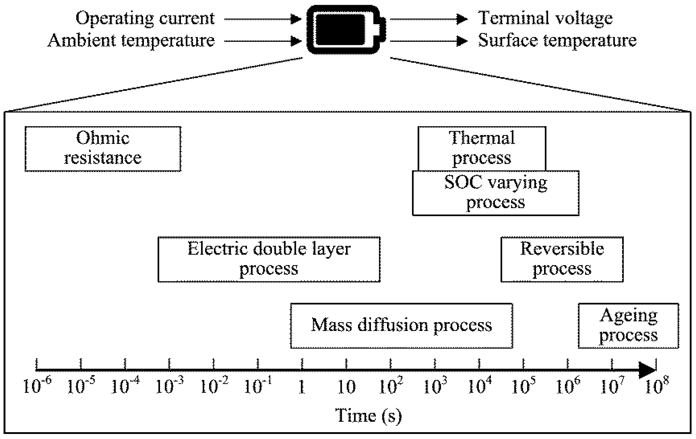
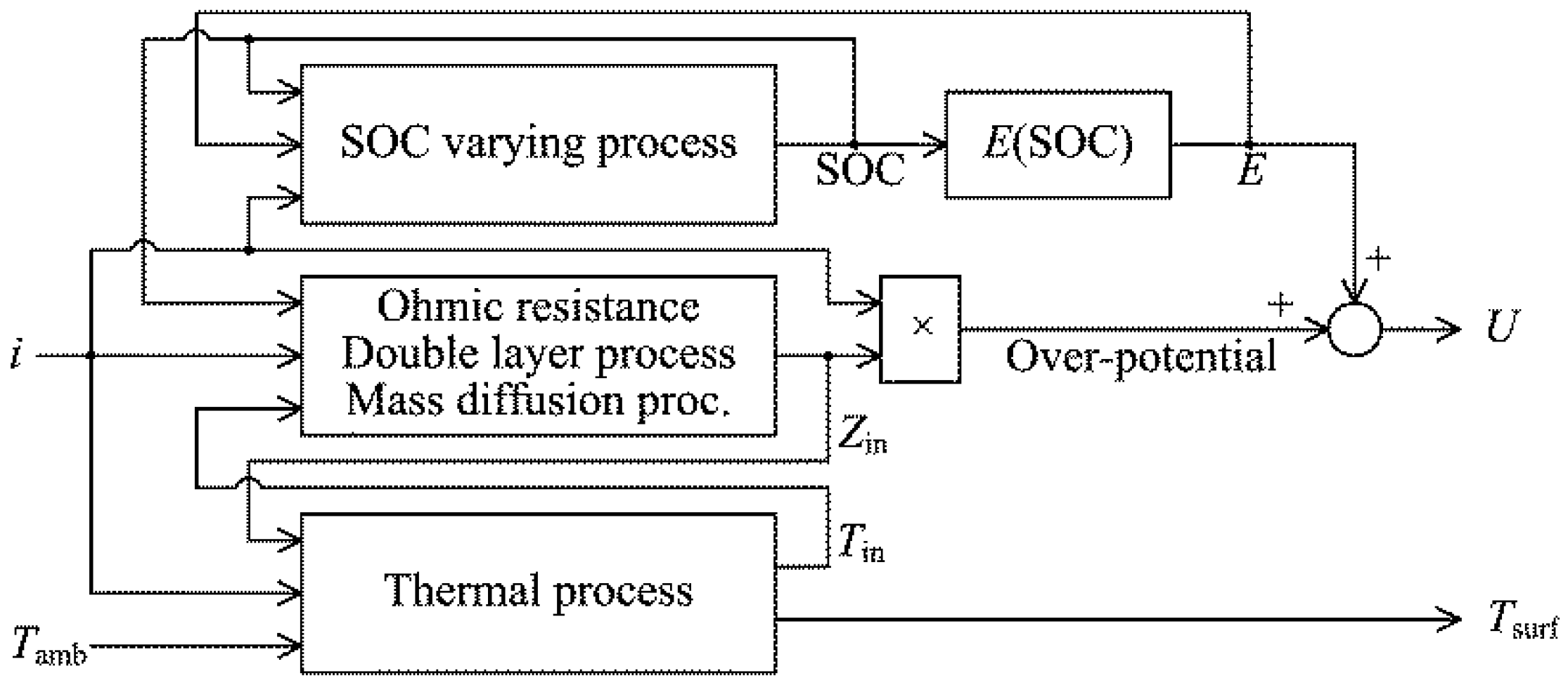
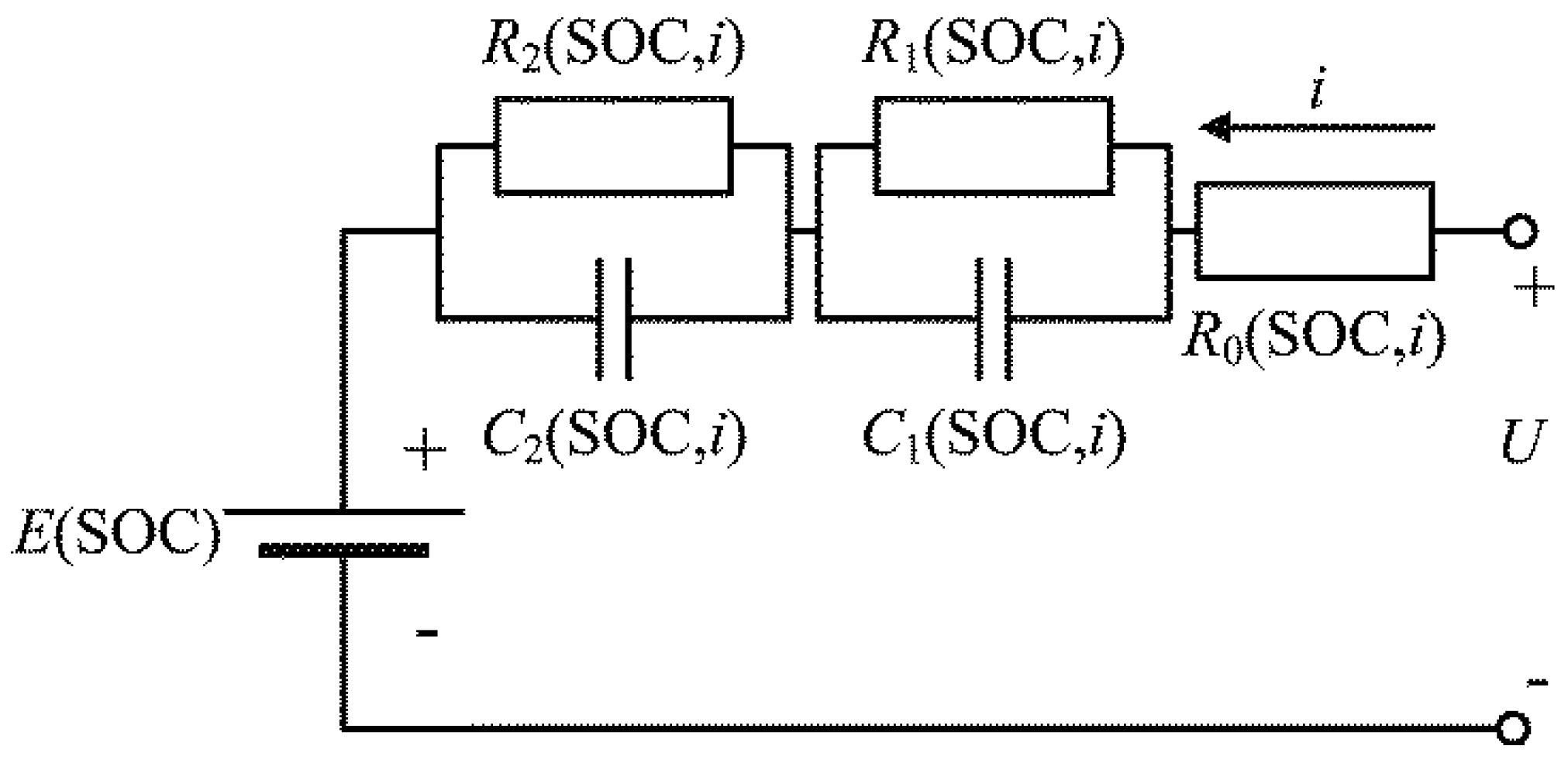
2. ECM Modification
3. Parameter Identification
3.1. Parameter Identification under a Set of {i1, i2, SOCj}
3.2. Parameter Identification under Different Sets of {i1, i2, SOCj}
3.3. Neglected Dynamics
4. Experiments and Analysis
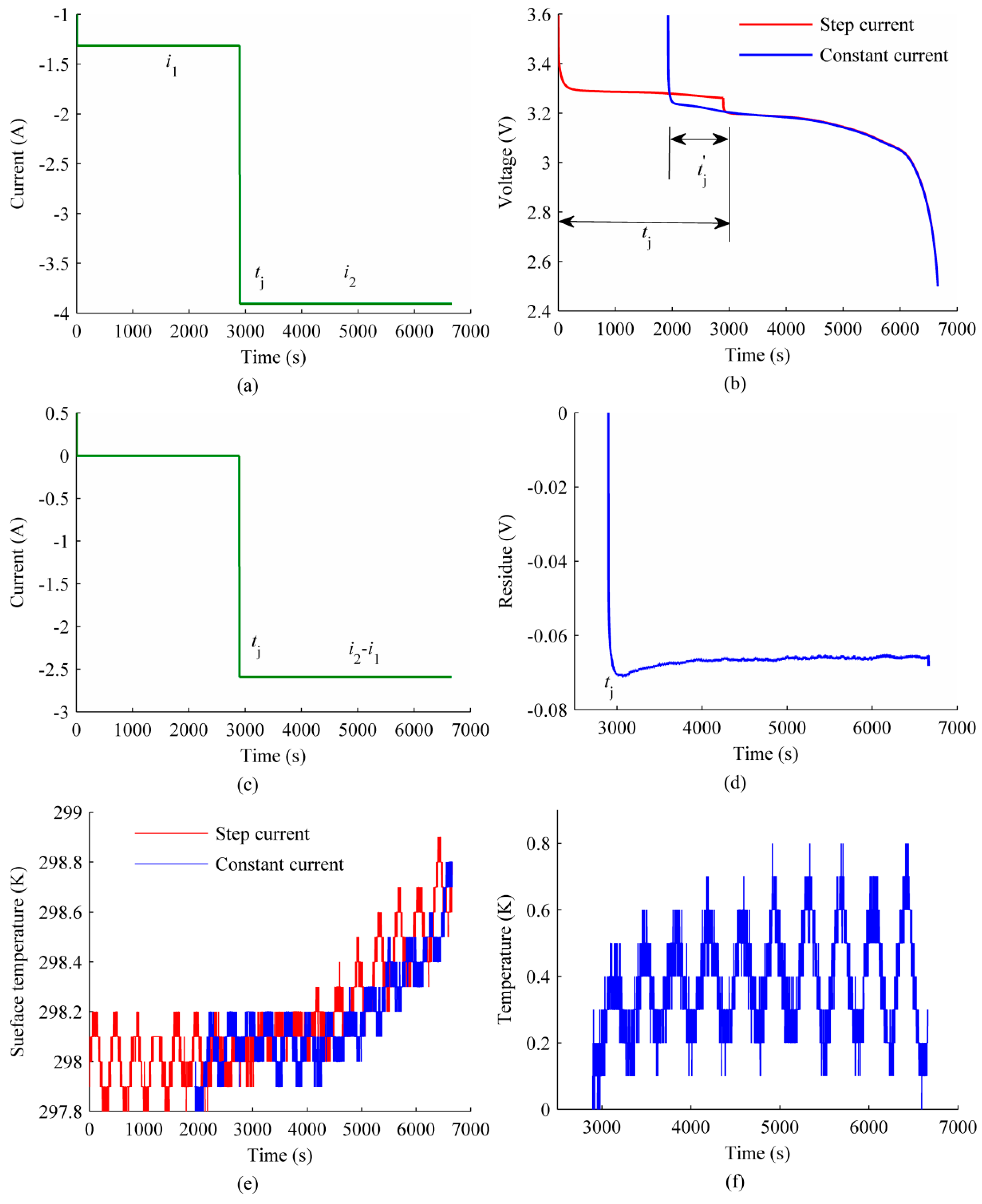
4.1. Test Conditions
4.2. Parameter Identification under a Set of {i1, i2, SOCj}
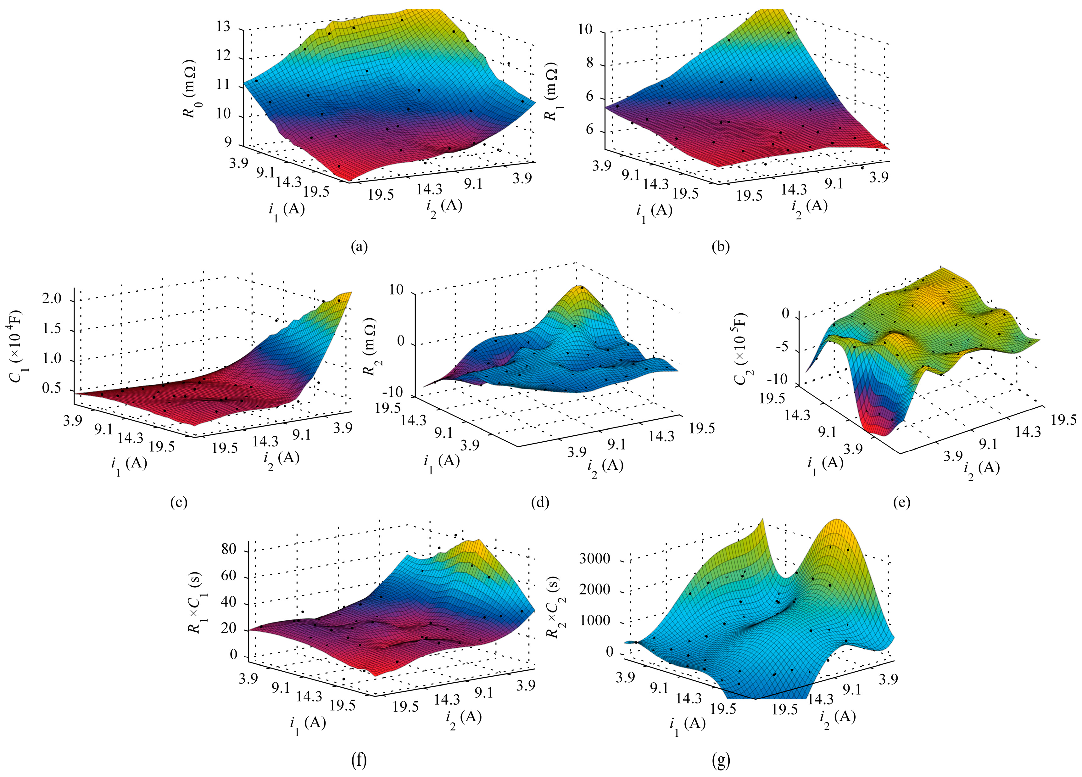
4.3. Parameter Identification under Different Sets of {i1, i2}
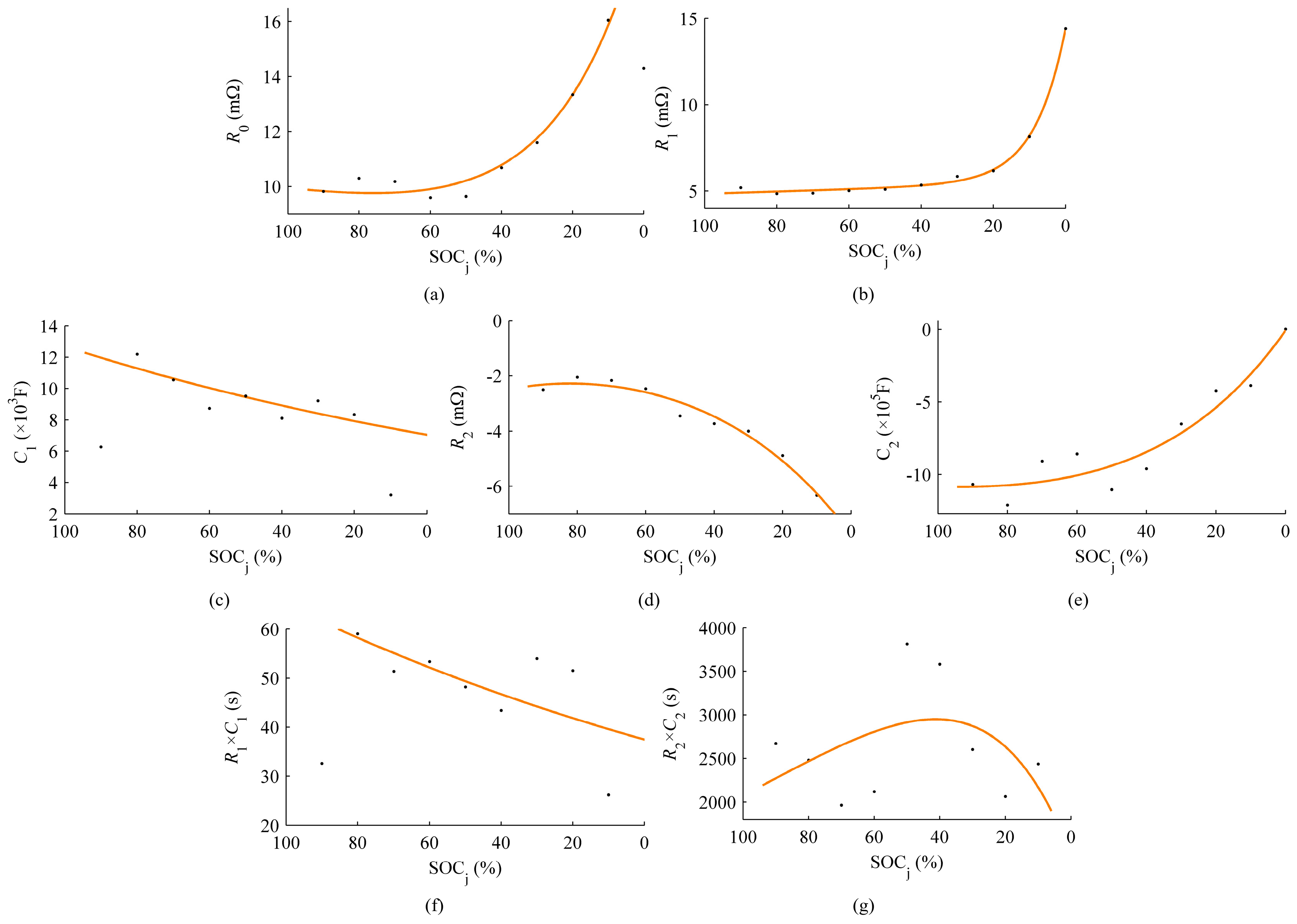
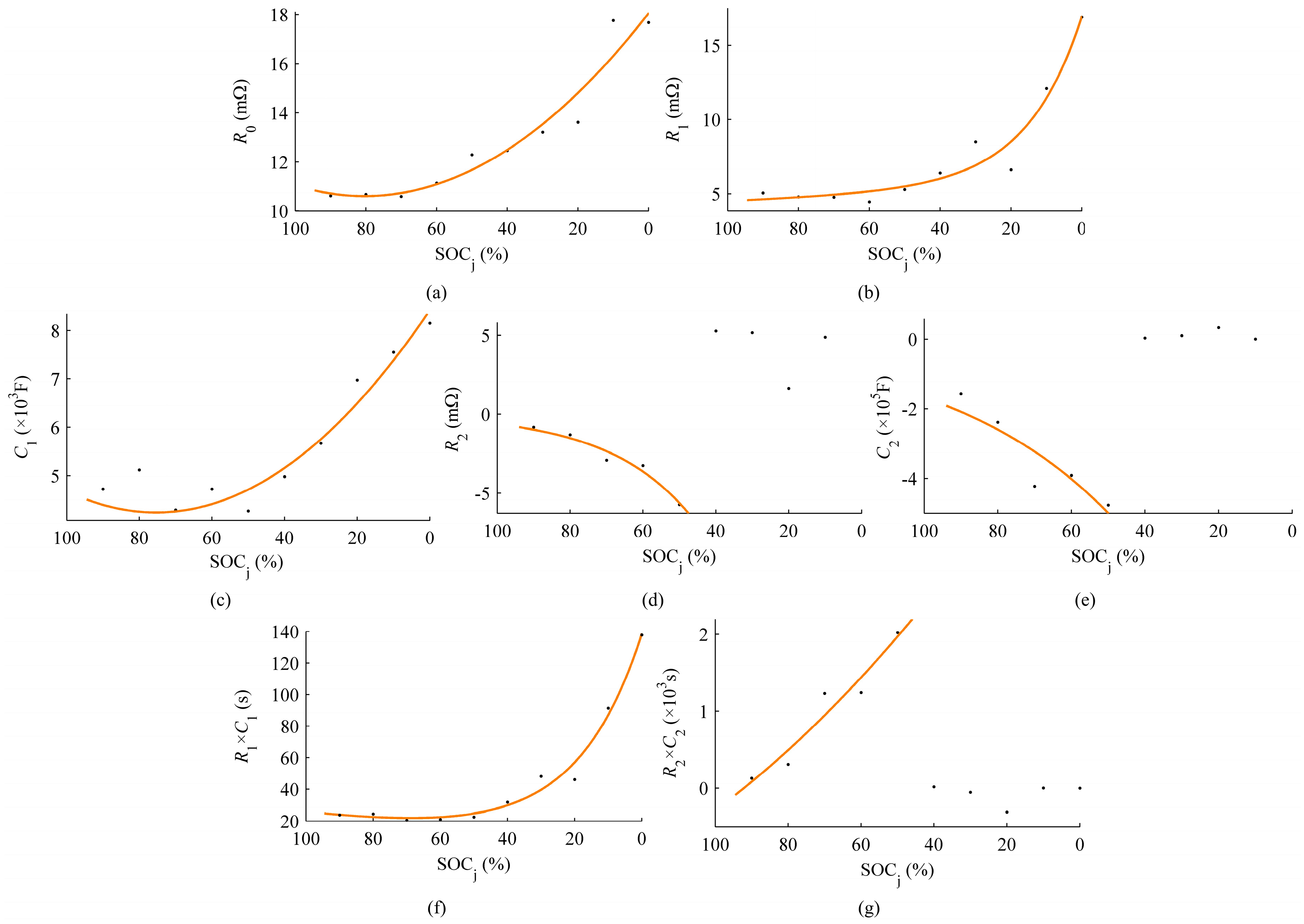
4.4. Parameter Identification under Different SOCj
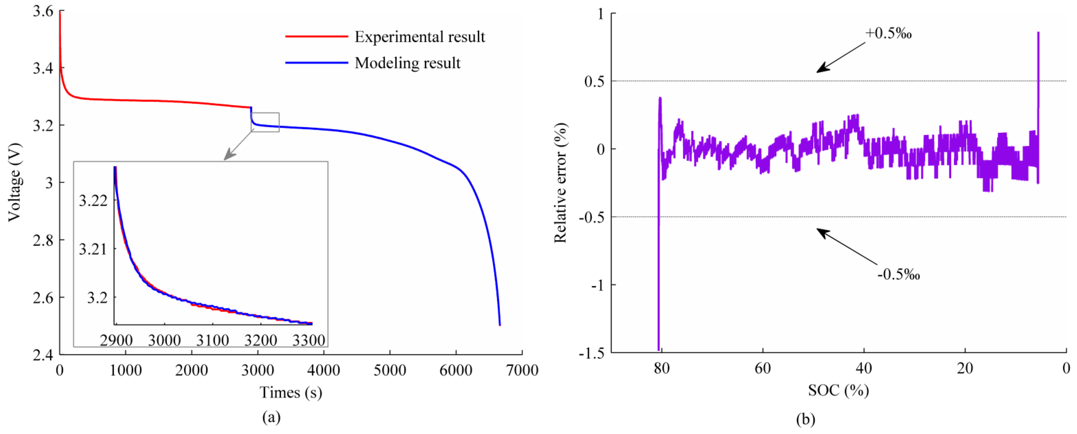
4.5. Verification under {i1 = −13 A, i2 = −10 A, SOCj = 71%}
5. Verification under DST (Dynamic Stress Test) and FUDS (Federal Urban Driving Schedule)
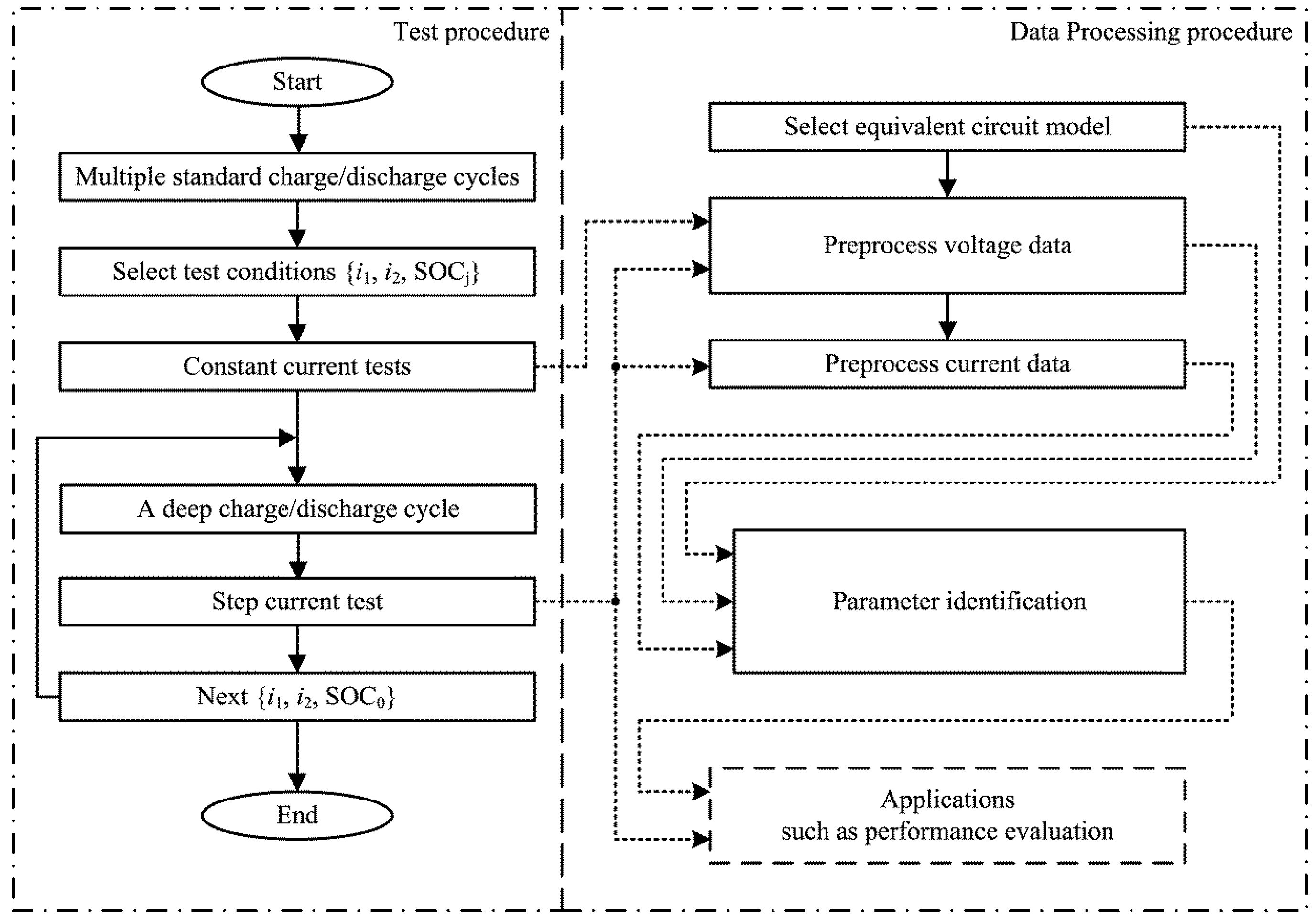
5.1. Data Processing Procedure under Multi-Transients Conditions
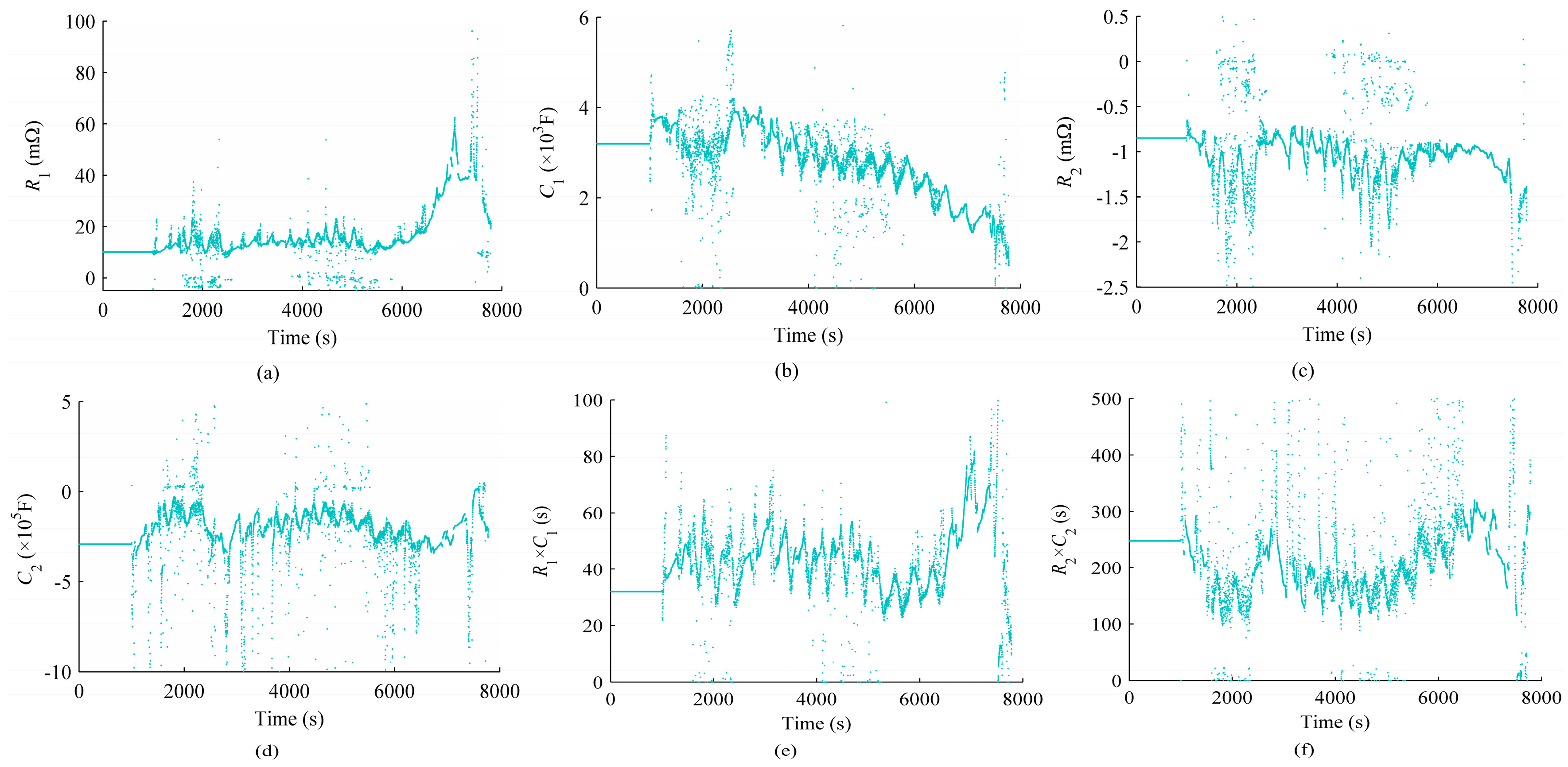
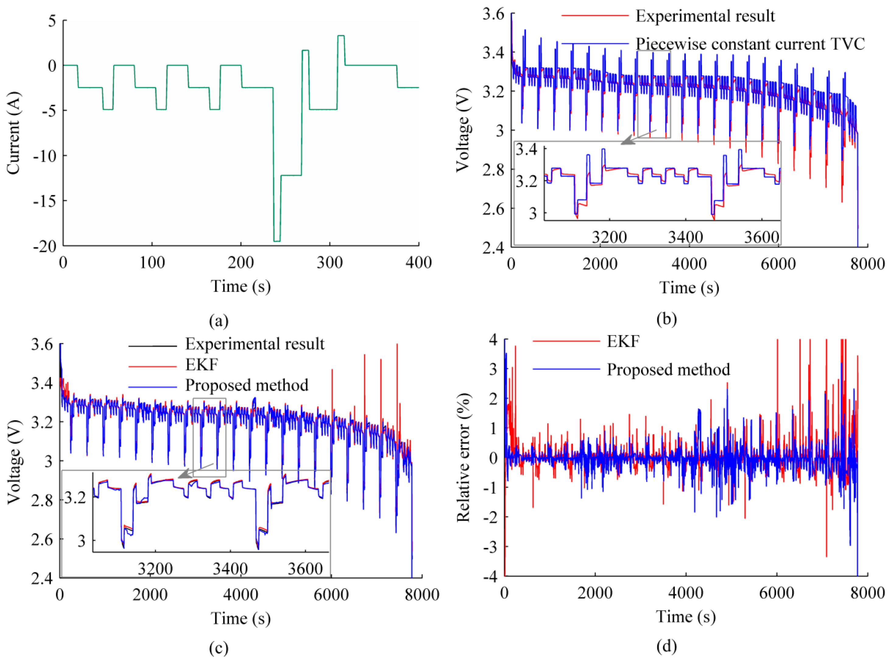
5.2. Verification under DST
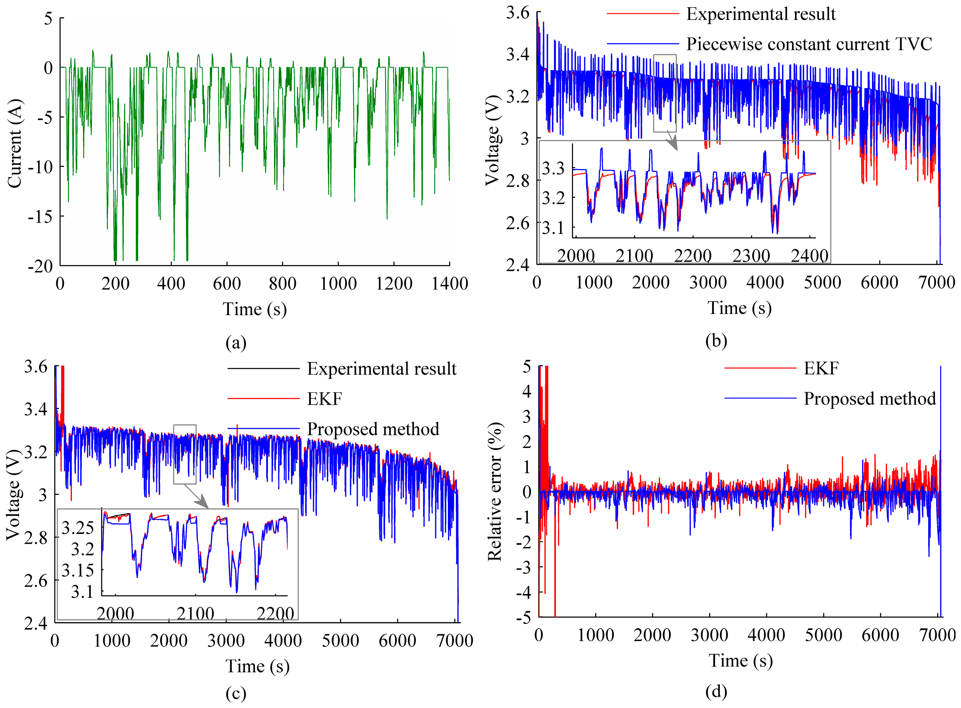
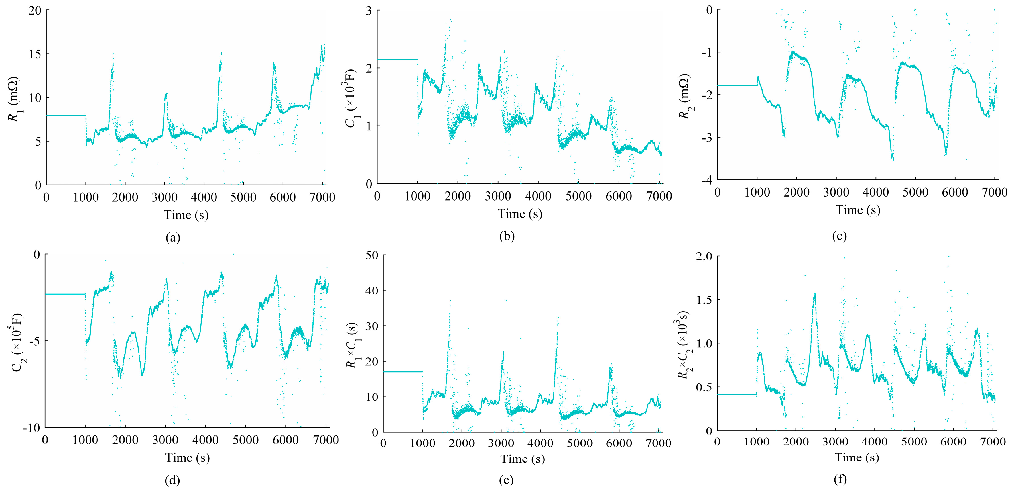
5.3. Verification under FUDS
6. Conclusions
- (1)
- An adequate test procedure is designed which includes step-change current tests and constant current tests. Therefore, battery dynamics can be sufficiently excited without introducing redundant excitations.
- (2)
- A corresponding data processing procedure is designed to extract battery dynamics including thermal process inherent in I-V characteristics, and then estimate the parameters of ECM, which are functions of current and SOC. Experimental results show that accuracy of the parameterization is sufficient.
Acknowledgments
Author Contributions
Conflicts of Interest
Appendix A. Derivation of Equation (9)
Appendix B. Derivation of Equation (10)
Appendix C. Procedure of Least Square Method
References
- Lu, L.; Han, X.; Li, J.; Hua, J.; Ouyang, M. A review on the key issues for lithium-ion battery management in electric vehicles. J. Power Sources 2013, 226, 272–288. [Google Scholar] [CrossRef]
- Jossen, A. Fundamentals of battery dynamics. J. Power Sources 2006, 154, 530–538. [Google Scholar] [CrossRef]
- Hu, X.; Li, S.; Peng, H. A comparative study of equivalent circuit models for Li-ion batteries. J. Power Sources 2012, 198, 359–367. [Google Scholar] [CrossRef]
- Abada, S.; Marlair, G.; Lecocq, A.; Petit, M.; Sauvant-Moynot, V.; Huet, F. Safety focused modeling of lithium-ion batteries: A review. J. Power Sources 2016, 306, 178–192. [Google Scholar] [CrossRef]
- Brand, J.; Zhang, Z.; Agarwal, R.K. Extraction of battery parameters of the equivalent circuit model using a multi-objective genetic algorithm. J. Power Sources 2014, 247, 729–737. [Google Scholar] [CrossRef]
- Li, J.; Wang, L.; Lyu, C.; Wang, H.; Liu, X. New method for parameter estimation of an electrochemical-thermal coupling model for LiCoO2 battery. J. Power Sources 2015, 307, 220–230. [Google Scholar] [CrossRef]
- Waag, W.; Fleischer, C.; Sauer, D.U. Critical review of the methods for monitoring of lithium-ion batteries in electric and hybrid vehicles. J. Power Sources 2014, 258, 321–339. [Google Scholar] [CrossRef]
- Feng, F.; Lu, R.; Zhu, C. A combined state of charge estimation method for lithium-ion batteries used in a wide ambient temperature range. Energies 2014, 7, 3004–3032. [Google Scholar] [CrossRef]
- Yuan, S.; Wu, H.; Yin, C. State of charge estimation using the extended Kalman filter for battery management systems based on the ARX battery model. Energies 2013, 4, 444–470. [Google Scholar] [CrossRef]
- Kim, D.; Koo, K.; Jeong, J.J.; Goh, T.; Kim, S.W. Second-order discrete-time sliding mode observer for state of charge determination based on a dynamic resistance Li-ion battery model. Energies 2013, 4, 5538–5551. [Google Scholar] [CrossRef]
- Zhang, X. Thermal analysis of a cylindrical lithium-ion battery. Electrochim. Acta 2011, 56, 1246–1255. [Google Scholar] [CrossRef]
- Guo, M.; Sikha, G.; White, R.E. Single-particle model for a lithium-ion cell: Thermal behavior. J. Electrochem. Soc. 2011, 158, A122–A132. [Google Scholar] [CrossRef]
- Prada, E.; Domenico, D.; Creff, Y.; Bernard, J.; Sauvant-Moynot, V.; Huet, F. Simplified electrochemical and thermal model of LiFePO4-graphite Li-ion batteries for fast charge applications. J. Electrochem. Soc. 2012, 159, A1508–A1519. [Google Scholar] [CrossRef]
- Guo, M.; Kim, G.; White, R.E. A three-dimensional multi-physics model for a Li-ion battery. J. Power Sources 2013, 240, 80–94. [Google Scholar] [CrossRef]
- Nieto, N.; Dіaz, L.; Gastelurrutia, J.; Alavam, I.; Blanco, F.; Ramos, J.C.; Rivas, A. Thermal Modeling of Large Format Lithium-Ion Cells. J. Electrochem. Soc. 2013, 160, A212–A217. [Google Scholar] [CrossRef]
- Yi, J.; Koo, B.; Shin, C.B. Three-Dimensional Modeling of the Thermal Behavior of a Lithium-Ion Battery Module for Hybrid Electric Vehicle Applications. Energies 2014, 7, 7856–7601. [Google Scholar] [CrossRef]
- Yazdanpour, M.; Taheri, P.; Mansouri, A.; Bahrami, M. A Distributed Analytical Electro-Thermal Model for Pouch-Type Lithium-Ion Batteries. J. Electrochem. Soc. 2014, 161, A1953–A1963. [Google Scholar] [CrossRef]
- Dees, D.; Gunen, E.; Abraham, D.; Jansen, A.; Prakash, J. Electrochemical Modeling of Lithium-Ion Positive Electrodes during Hybrid Pulse Power Characterization Tests. J. Electrochem. Soc. 2008, 155, A603–A613. [Google Scholar] [CrossRef]
- Albertus, P.; Christensen, J.; Newman, J. Experiments on and Modeling of Positive Electrodes with Multiple Active Materials for Lithium-Ion Batteries. J. Electrochem. Soc. 2009, 156, A606–A618. [Google Scholar] [CrossRef]
- Srinivasan, V.; Newman, J. Design and Optimization of a Natural Graphite/Iron Phosphate Lithium-Ion Cell. J. Electrochem. Soc. 2004, 151, A1530–A1538. [Google Scholar] [CrossRef]
- Doyle, M.; Fuentes, Y. Computer Simulations of a Lithium-Ion Polymer Battery and Implications for Higher Capacity Next-Generation Battery Designs. J. Electrochem. Soc. 2003, 150, A706–A713. [Google Scholar] [CrossRef]
- Zhu, J.G.; Sun, Z.C.; Wei, X.Z.; Dai, H.F. A new lithium-ion battery internal temperature on-line estimate method based on electrochemical impedance spectroscopy measurement. J. Power Sources 2015, 274, 990–1004. [Google Scholar] [CrossRef]
- Gomez, J.; Nelson, R.; Kalu, E.; Weatherspoon, M.H.; Zheng, J.P. Equivalent circuit model parameters of a high-power Li-ion battery: Thermal and state of charge effects. J. Power Sources 2011, 196, 4826–4831. [Google Scholar] [CrossRef]
- Lin, X.; Perez, H.E.; Mohan, S.; Siegel, J.B.; Stefanopoulou, A.G.; Ding, Y.; Castanier, M.P. A lumped-parameter electro-thermal model for cylindrical batteries. J. Power Sources 2014, 257, 1–11. [Google Scholar] [CrossRef]
- Murashko, K.; Pyrhönen, J.; Laurila, L. Three-dimensional thermal model of a lithium ion battery for hybrid mobile working machines: Determination of the model parameters in a pouch cell. IEEE Trans. Energy Convers. 2013, 28, 335–343. [Google Scholar] [CrossRef]
- Alaoui, C. Solid-state thermal management for lithium-ion EV batteries. IEEE Trans. Veh. Technol. 2013, 62, 98–107. [Google Scholar] [CrossRef]
- Vertiz, G.; Oyarbide, M.; Macicior, H.; Miguel, O.; Cantero, I.; Arroiabe, P.F.; Ulacia, I. Thermal characterization of large size lithium-ion pouch cell based on 1d electro-thermal model. J. Power Sources 2014, 272, 476–484. [Google Scholar] [CrossRef]
- Lithium Ion Cells and Batteries Used in Portable Electronic Equipments: Safety Requirements; GB 31241-2014; Standards Press of China: Beijing, China, 2014.
- Wu, B.; Yufit, V.; Marinescu, M.; Offer, G.J.; Martinez-Botas, R.F.; Brandon, N.P. Coupled thermal electrochemical modelling of uneven heat generation in lithium-ion battery packs. J. Power Sources 2013, 243, 544–554. [Google Scholar] [CrossRef]
- Buller, S.; Thele, M.; Karden, E. Impedance-based non-linear dynamic battery modeling for automotive applications. J. Power Sources 2003, 113, 422–430. [Google Scholar] [CrossRef]
- Andre, D.; Meiler, M.; Steiner, K.; Wimmer, Ch.; Soczka-Guth, T.; Sauer, D.U. Characterization of high-power lithium-ion batteries by electrochemical impedance spectroscopy I: Experimental investigation. J. Power Sources 2011, 196, 5334–5341. [Google Scholar] [CrossRef]
- Andre, D.; Meiler, M.; Steiner, K.; Wimmer, Ch.; Soczka-Guth, T.; Sauer, D.U. Characterization of high-power lithium-ion batteries by electrochemical impedance spectroscopy II: Modelling. J. Power Sources 2011, 196, 5349–5356. [Google Scholar] [CrossRef]
- Schmidt, J.P.; Chrobak, T.; Ender, M.; Illig, J.; Klotz, D.; Ivers-Tiffée, E. Studies on LiFePO4 as cathode material using impedance spectroscopy. J. Power Sources 2011, 196, 5342–5348. [Google Scholar] [CrossRef]
- Fleischer, C.; Waag, W.; Heyn, H.M.; Sauer, D.U. On-line adaptive battery impedance parameter and state estimation considering physical principles in reduced order equivalent circuit battery models: Part 1. Requirements critical review of methods and modeling. J. Power Sources 2014, 260, 276–291. [Google Scholar] [CrossRef]
- Fleischer, C.; Waag, W.; Heyn, H.M.; Sauer, D.U. On-line adaptive battery impedance parameter and state estimation considering physical principles in reduced order equivalent circuit battery models: Part 2. Parameter and state estimation. J. Power Sources 2014, 262, 457–482. [Google Scholar] [CrossRef]
- Roscher, M.A.; Sauer, D.U. Dynamic electric behavior and open-circuit-voltage modeling of LiFePO4-based lithium ion secondary batteries. J. Power Sources 2011, 196, 331–336. [Google Scholar] [CrossRef]
- Chiang, Y.H.; Sean, W.Y.; Ke, J.C. Online estimation of internal resistance and open-circuit voltage of lithium-ion batteries in electric vehicles. J. Power Sources 2011, 196, 3921–3932. [Google Scholar] [CrossRef]
- Roscher, M.A.; Assfalg, J.; Bohlen, O.S. Detection of utilizable capacity deterioration in battery systems. IEEE Trans. Veh. Technol. 2011, 60, 98–103. [Google Scholar] [CrossRef]
- He, H.; Xiong, R.; Zhang, X.; Sun, F.; Fan, J. State-of-charge estimation of the lithium-ion battery using an adaptive extended Kalman filter based on an improved Thevenin model. IEEE Trans. Veh. Technol. 2011, 60, 1461–1469. [Google Scholar]
- Pattipati, B.; Sankavaram, C.; Pattipati, K.R. System identification and estimation framework for pivotal automotive battery management system characteristics. IEEE Trans. Syst. Man Cybern. Part C Appl. Rev. 2011, 41, 869–884. [Google Scholar] [CrossRef]
- Electric Vehicle Battery Test Procedures Manual. Available online: http://avt.inl.gov/battery/pdf/usabc_manual_rev2.pdf (accessed on 2 December 2015).
- Battery Test Manual or Plug-In Hybrid Electric Vehicles. Available online: https://inldigitallibrary.inl.gov/sti/3952791.pdf (accessed on 1 June 2016).
- Negative Resistance. Available online: https://en.wikipedia.org/wiki/Negative_resistance (accessed on 13 March 2016).
- Grassi, R.; Gnudi, A.; Lecce, V.D.; Gnani, E.; Reggiani, S.; Baccarani, G. Exploiting negative differential resistance in monolayer graphene FETs for high voltage gains. IEEE Trans. Electron. Devices 2014, 61, 617–624. [Google Scholar] [CrossRef]
- Ershov, M.; Liu, H.C.; Buchanan, M.; Wasilewski, Z.R.; Jonscher, A.K. Negative capacitance effect in semiconductor devices. IEEE Trans. Electron. Devices 1998, 45, 2196–2206. [Google Scholar] [CrossRef]
- Negative Impedance Converter. Available online: https://en.wikipedia.org/wiki/Negative_impedance_converter (accessed on 21 April 2016).
- Jain, A.; Alam, M.A. Stability constraints define the minimum subthreshold swing of a negative capacitance field-effect transistor. IEEE Trans. Electron. Devices 2014, 61, 2235–2242. [Google Scholar] [CrossRef]
- Bard, A.J.; Faulkner, L.R. Electrochemical Methods: Fundamentals and Applications, 2nd ed.; John Wiley & Sons Inc.: New York, NY, USA, 2001; pp. 161–168. [Google Scholar]
- Hu, Y.; Yurkovich, S. Linear parameter varying battery model identification using subspace methods. J. Power Sources 2011, 196, 2913–2923. [Google Scholar] [CrossRef]
- Garnier, H.; Mensler, M.; Richard, A. Continuous-time model identification from sampled data: Implementation issues and performance evaluation. Int. J. Control 2003, 76, 1337–1357. [Google Scholar] [CrossRef]


| Item | Value |
|---|---|
| Battery parameters | - |
| Type and Batch No. | BAK 36800MP-Fe/2VF10L06 06877 |
| Rated capacity (Ah) | 6.5 |
| Rated temperature (K) | 298 |
| Maximum charge current (A) | 3.25 |
| Maximum discharge current (A) | −19.5 |
| Test environment | - |
| Test bench type | Neware CT-4008-5V100A-NTFA |
| Measurement range | 0.01–5 V, 0.2–100 A |
| Measurement accuracy (%) | ±0.0153 |
| Sample rate (Hz) | 1 |
| Thermal chamber type | Jianhu JH-150F |
| Accuracy (K) | ±1 |
| Operating conditions | - |
| i1 and i2 (A) | 1.3, 3.9, 6.5, 9.1, 11.7, 14.3, 16.9, 19.5 |
| SOCj (%) | 10, 20, 30, 40, 50, 60, 70, 80, 90, 100 |
| Ambient temperature (K) | 298 |
| Item | Optimal Value | Estimated Value | Relative Error (%) |
|---|---|---|---|
| R0 (mΩ) | 10.803 | 10.733 | −0.648 |
| R1 (mΩ) | 4.236 | 4.257 | 0.496 |
| C1 (×103 F) | 6.156 | 6.707 | 8.591 |
| R1 × C1 (s) | 26.077 | 28.552 | 9.491 |
| R2 (mΩ) | −2.349 | −2.692 | 14.602 |
| C2 (×105 F) | −2.634 | −1.914 | −27.335 |
| R2 × C2 (s) | 618.734 | 515.214 | −16.731 |
© 2016 by the authors; licensee MDPI, Basel, Switzerland. This article is an open access article distributed under the terms and conditions of the Creative Commons Attribution (CC-BY) license (http://creativecommons.org/licenses/by/4.0/).
Share and Cite
He, Z.; Yang, G.; Lu, L. A Parameter Identification Method for Dynamics of Lithium Iron Phosphate Batteries Based on Step-Change Current Curves and Constant Current Curves. Energies 2016, 9, 444. https://doi.org/10.3390/en9060444
He Z, Yang G, Lu L. A Parameter Identification Method for Dynamics of Lithium Iron Phosphate Batteries Based on Step-Change Current Curves and Constant Current Curves. Energies. 2016; 9(6):444. https://doi.org/10.3390/en9060444
Chicago/Turabian StyleHe, Zhichao, Geng Yang, and Languang Lu. 2016. "A Parameter Identification Method for Dynamics of Lithium Iron Phosphate Batteries Based on Step-Change Current Curves and Constant Current Curves" Energies 9, no. 6: 444. https://doi.org/10.3390/en9060444