Development and a Validation of a Charge Sensitive Organic Rankine Cycle (ORC) Simulation Tool ^†

Abstract

Despite the increasing interest in organic Rankine cycle (ORC) systems and the large number of cycle models proposed in the literature, charge-based ORC models are still almost absent. In this paper, a detailed overall ORC simulation model is presented based on two solution strategies: condenser subcooling and total working fluid charge of the system. The latter allows the subcooling level to be predicted rather than specified as an input. The overall cycle model is composed of independent models for pump, expander, line sets, liquid receiver and heat exchangers. Empirical and semi-empirical models are adopted for the pump and expander, respectively. A generalized steady-state moving boundary method is used to model the heat exchangers. The line sets and liquid receiver are used to better estimate the total charge of the system and pressure drops. Finally, the individual components are connected to form a cycle model in an object-oriented fashion. The solution algorithm includes a preconditioner to guess reasonable values for the evaporating and condensing temperatures and a main cycle solver loop which drives to zero a set of residuals to ensure the convergence of the solution. The model has been developed in the Python programming language. A thorough validation is then carried out against experimental data obtained from two test setups having different nominal size, working fluids and individual components: (i) a regenerative ORC with a 5 kW scroll expander and an oil flooding loop; (ii) a regenerative ORC with a 11 kW single-screw expander. The computer code is made available through open-source dissemination.

1. Introduction

The investigation of organic Rankine cycles (ORCs) both numerically and experimentally [1,2,3,4,5] has seen a rapid growth in the last years due to increasing concerns about the environment and the Earth’s limited fossil fuel resources. Exploiting low temperature heat sources from industrial waste heat or other renewable energies such as solar and geothermal by means of ORC systems has been widely demonstrated to be a viable solution to generate electricity [6].

Numerical simulations play an essential role in the analysis of ORC systems because of the variety of boundary conditions imposed by heat sources, cold sinks, and different applications. The optimization of an ORC unit is the result of a thermodynamic analysis [7], a fluid selection process [8], the sizing of the components [9,10] and ultimately a thermo-economic analysis [11]. In many cases, feasibility studies as well as potential improvements in terms of cycle architectures (e.g., transcritical, supercritical, etc.) [12] and novel working fluids (e.g., hydrocarbons, zeotropic mixtures, etc.) rely exclusively on numerical simulations. The number of published papers [13] dealing with organic Rankine cycles in recent years is plotted in Figure 1. By considering ‘simulation’ and ‘optimization’ as search keywords, the related number of papers has grown four to five times in a time span of almost 7 years.

Different modeling approaches, both steady-state and dynamic have been proposed in the open literature. Regarding steady-state models, the most common approach for ORC systems is a simplified thermodynamic analysis. In particular, assumptions are made regarding the degrees of subcooling at the condenser outlet (or pump inlet) and superheating at the evaporator outlet (or expander inlet), as well as the evaporating and condensing temperatures (or pressures). It is a common choice to assume a constant value for the isentropic efficiency of the pump and expander and to assume the compression and the expansion to be adiabatic. The cycle is solved by calculating the relevant thermodynamic states of the cycle and the performance of the system in terms of power produced at the expander and the overall cycle efficiency. Second Law analysis is also performed to assess exergy losses [14]. This type of simplified modeling is useful as a preliminary investigation of the effect of working fluids and operating conditions on the cycle performance trends. In fact, this methodology represents a typical working fluid screening method or an objective function to be optimized given a set of desired working conditions. However, the physical characteristics and behavior of any real system components are not taken into account. Therefore, it is not possible to accurately predict the off-design performance of a particular system.

Despite the large number of papers dealing with ORC modeling, little attention has been given to detailed ORC modeling. Quoilin et al. [15] developed a detailed simulation model of an ORC including separate models for each cycle component. The condenser and evaporator were modeled by a means of the effectiveness-NTU method for counter flow heat exchangers. The heat exchangers were divided into three zones, each of them characterized by proper heat transfer correlations. Single-phase forced convection heat transfer, boiling and condensation correlations were calibrated on experimental data. A semi-empirical model of the scroll expander was also included, featuring friction losses, heat transfer, intake throttling and internal leakage. A simple pump model based on its swept volume and its global isentropic efficiency was used. The overall cycle model was obtained by connecting the different sub-models in the EES (Engineering Equation Solver) environment [16]. Sun and Li [17] presented a detailed analysis of an ORC using R134a as the working fluid. The expander and the pump were modeled with two empirical correlations based on the performance maps given by the manufacturer. Affinity law was applied to obtain the pump power consumption at different rotational speeds. A discretized heat exchanger model was applied to the evaporator and condenser. The condenser was assumed to be air cooled and the fan power consumption was also taken into account. An optimization algorithm was implemented in order to obtain the optimal set of operating variables to maximize either the system net power generation or the system thermal efficiency. The controlled variables were the working fluid mass flow rate, the mass flow rate of the air cooled condenser, and the expander inlet pressure. However, both models were not fully deterministic because the subcooling level at the condenser outlet was specified and not calculated [1]. The prediction of the subcooling is related to the refrigerant charge model which, for ORC systems, has not been fully developed yet.

Charge-sensitive detailed models have been extensively used in vapor compression cooling and heat pumping for design and diagnostic purposes. It is worth mentioning that one of the first detailed vapor compression cycle models was published by Hiller and Glicksman in 1976 [18]. This comprehensive model based on several subroutines included a moving boundary model for the heat exchangers, single and two-phase pressure drops, oil entrainment in suction and discharge risers, liquid line flashing, moisture removal on the evaporator side, refrigerant-oil solubility, oil circulation, compressor load effect on motor efficiency, motor cooling effect on compressor, compressor valve dynamics and friction losses. In later academic research, a charge-sensitive vapor compression cycle model was initially developed by Rossi [19] with the aim to develop techniques for automated fault detection and diagnostics in vapor compression equipment. The simulation tool named ACMODEL included four main component models, i.e., compressor, condenser, evaporator and the expansion device. Four interconnecting line models were also included. The solution algorithm was based on three residuals: the total refrigerant charge in the system, the enthalpy difference between the inlet of the distribution tubes and the expansion device outlet and the pressure difference between liquid line outlet and expansion device inlet. The simulation tool has been successively updated by Shen [20,21] to include an improved tuning method for charge simulations to allow more precise prediction of the effect of different charge levels over a wide range of operating conditions. The effects of small percentages of lubricant contained in the refrigerant flow on the system performance were also investigated.

Many of the issues investigated on vapor compression cycles apply also to ORC systems, i.e., the presence of lubricant oil in the system, two-phase flow conditions, working fluid charge, subcooling and superheating, among others. In fact, it is well known that the working charge affects the performance of ORC systems and it represents a non-negligible cost especially for larger units. In order to optimize the operation of an ORC unit, the effect of different charge levels in the system under design and off-design conditions should be predicted.

Last but not least, only a few commercial simulation packages, i.e., Cycle-Tempo, are available online and developed also for ORC systems. If the search is restricted to open-source tools, the availability is further reduced. For example, the Thermodynamics Laboratory at University of Liege created two significant tools: “SimORC” for the steady state simulation of ORC based on EES featuring a Graphical User Interface (GUI) and “Thermocycle’ an open-source Modelica based library for the dynamic simulation of ORC systems.

The aim of the present work is to propose the first detailed ORC model which can be solved based on the working fluid charge level. The option to solve based on the subcooling level, which represents the more common modeling approach, is also included. Such a model is useful for cycle performance prediction of real units and as a starting point for further fault detection and diagnostic analyses applied to ORCs. Furthermore, the simulation code is made available open-source.

In the first part of this paper, a charge-based ORC framework, named “ORCSim”, is presented and described with emphasis on the solution strategies. Each component of the ORC system is described and the general solution algorithm is explained. The simulation code has been implemented in the open-source Python programming language. In the second part, the components and the cycle models are validated with experimental results obtained with two different ORC systems running with different working fluids and different types of components. Additional results are also proposed regarding the charge-based solver.

2. Detailed Cycle Modeling: ORCSim

This section describes in detail the overall architecture of the simulation model as well as each independent component model of which the cycle model is composed. The most general case of an ORC with internal heat exchanger is considered in this section.

The following constraints have been considered during the development of the model:

• the working fluid mass flow rate is imposed by the pump (either the rotational speed or the frequency can be used as input);
• the evaporating temperature is related to the pump outlet pressure and the pressure drop between pump and the evaporator;
• the superheating is imposed by the evaporator for a fixed expander rotational speed;
• the condensing pressure is imposed by the condenser;
• the subcooling level at the condenser outlet can be specified as an input or predicted by introducing a refrigerant charge model. In the latter case, the ORC model is charge-based;
• an internal heat exchanger (or regenerator) can be included in the simulation if desired;
• the effect of solubility of refrigerant vapor in the lubricant oil is considered only in the oil separator, where solubility data is available. During the expansion process, the solubility is neglected since the enthalpy of mixing is small compared to the change of enthalpy through the expander.

The independent models considered are the refrigerant pump, the expander, the plate heat exchangers, the liquid receiver, the line sets and the oil separator. Different modeling approaches have been considered in order to provide different levels of complexity to the cycle model and to guarantee a more numerically robust code. Empirical models have been applied to characterize the pumps (centrifugal and volumetric) and the expander. Only positive displacement expanders are considered at the moment. A semi-empirical model which accounts for the presence of oil has been developed for the expander. The form of this expander model has been proven to be applicable for a wide range of positive displacement machines (either compressors or expanders) [22,23,24]. A deterministic model of the heat exchangers which makes use of a general moving boundary scheme has been adopted for all the plate heat exchangers. The main reasons behind this choice of model are its robustness and computational efficiency, its capability to handle all the possible combinations of liquid, two-phase and vapor zones and the possibility to calculate the charge level in the heat exchanger. The solution algorithm schemes are also explained with particular focus on the charge based solver. The models described in the following have been implemented in the Python programming language. An example of the detailed ORC model in the Python programming language (ORCSim) can be found in the ORCmKit library [25].

2.1. Thermo-Physical Property Wrappers

Most of the computational effort of a detailed cycle model takes place while retrieving and evaluating the properties of the working fluids. Therefore, the property wrapper must combine computational efficiency with accuracy and a sufficiently broad database of fluids.

Both CoolProp 5.1.2 [26] and REFPROP 9.1 [27] have been included within the detailed ORC model to cover the most common ORC applications in terms of refrigerant working fluids and their mixtures, as well as hot and cold source fluids, compressible and incompressible. In particular, incompressible fluids such as thermal oils or coolants are only available in CoolProp. A modified version of the Refprop2.py [28] has been implemented which allows us to call the properties from REFPROP with the same syntax as in CoolProp. For consistency with CoolProp, the PropsSI function has been used, with only SI units. The possibility to call refrigerant mixture properties based on mass fraction has also been added to the original version of Refprop2.py.

Positive displacement expanders require lubrication to ensure the correct running of the rotating parts and to reduce the internal leakage paths. To the authors’ knowledge, lubricant oil property libraries are not readily available open-source. An additional property wrapper has been added to calculate both the properties of the lubricant oil and the mixture of oil and refrigerant. Many of the oil properties were obtained from [29]. To simplify the analysis, the mixture has been treated as a pseudo-pure fluid, i.e., an ideal mixture model has been used. For a homogeneous mixture of two components with equal velocities, mixture properties such as specific enthalpy, specific entropy, specific internal energy and exergy, the specific volume, and the mixture constant pressure specific heat can be calculated by introducing an oil mass fraction, $x_{oil}$. For example the mixture specific enthalpy is given by:

$$h_{mix}=x_{oil}{h}_{oil}\left(T_{oil}\right)+\left(1-x_{oil}\right)h_r\left(T_r,p_r\right)$$

(1)

The other aforementioned properties can be calculated in a similar fashion. The mixture density and mixture thermal conductivity are calculated based on a void fraction weighted average correlation:

$$\begin{array}{cc}\hfill {\rho }_{mix}& =\alpha {\rho }_r+\left(1-\alpha \right){\rho }_{oil}\hfill \end{array}$$

(2)

$$\begin{array}{cc}\hfill k_{mix}& =\alpha k_r+\left(1-\alpha \right)k_{oil}\hfill \end{array}$$

(3)

where the homogeneous void fraction, α is given by:

$$\alpha =\frac{1}{1+\left[\frac{1}{x_r}-1\right]S\frac{{\rho }_r}{{\rho }_{oil}}}$$

(4)

with the slip ratio S equal to unity. Many correlations exist to calculate the mixture viscosity. Two models have been implemented. The first one is based on the model proposed by McAdams [30]:

$${\mu }_{mix}={\left(\frac{x_{oil}}{{\mu }_{oil}}+\frac{x_r}{{\mu }_r}\right)}^{-1}$$

(5)

The second one is the correlation developed by Dukler et al. [31] based on the mass averaged value of the kinematic viscosity:

$${\mu }_{mix}={\rho }_{mix}\left[x_r\frac{{\mu }_r}{{\rho }_r}+x_{oil}\frac{{\mu }_{oil}}{{\rho }_{oil}}\right]$$

(6)

The solubility of refrigerants in lubricant oils is also included and is discussed further in Section 2.7.

2.2. Plate Heat Exchanger Model

The heat exchangers of the overall ORC model (typically evaporator, condenser and regenerator) are modeled with a general steady-state moving boundary approach. In this work only plate heat exchangers (PHEX) are considered. However, the model can be readily adapted to other types of heat exchangers by modifying the geometric parameters and heat transfer and pressure drop correlations. The model is nearly identical to the one proposed by Bell et al. [32] and available open-source within the ACHP project, version 1.5.0 [33]. In the following the general algorithm of the model is briefly described and the modifications highlighted.

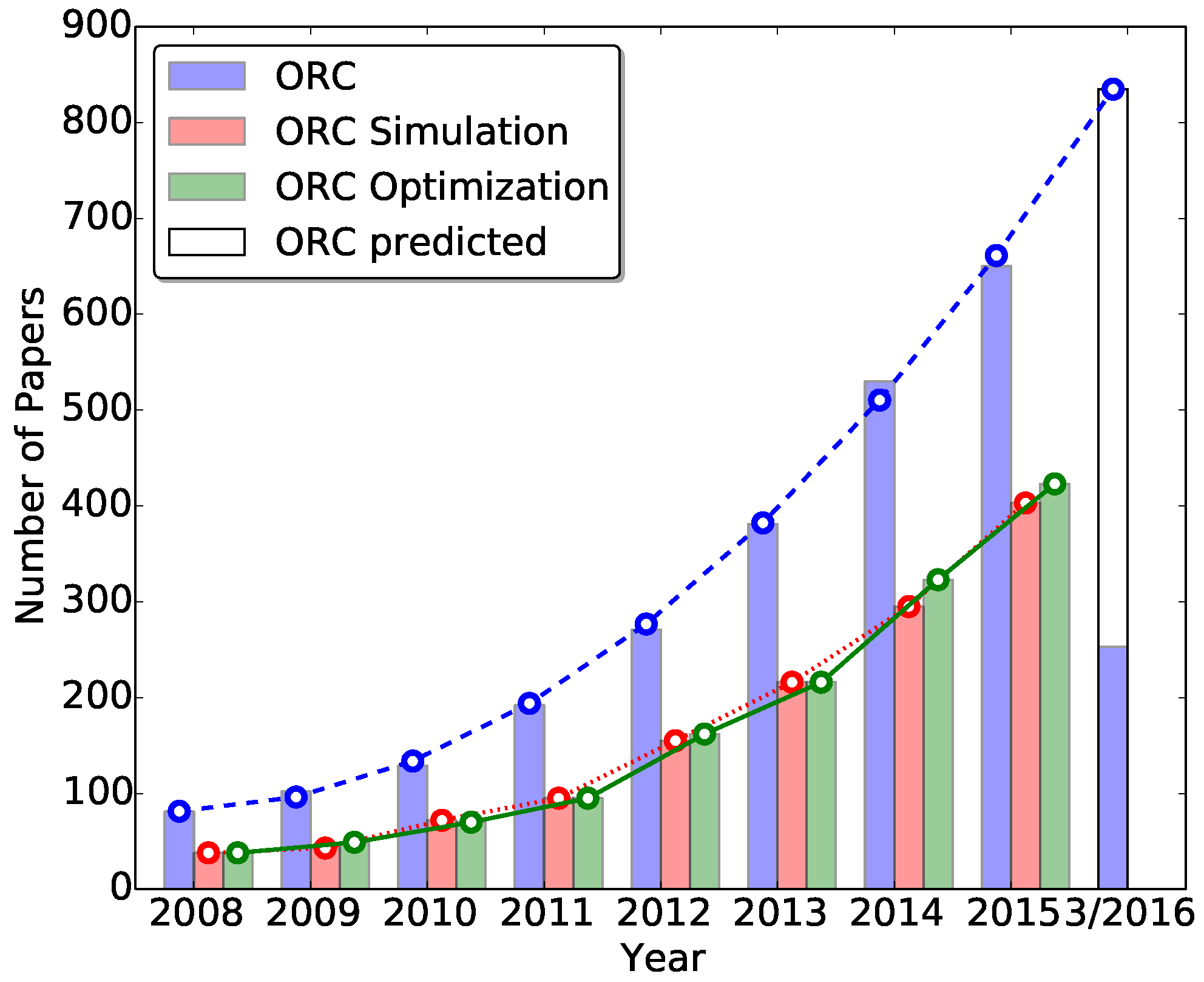
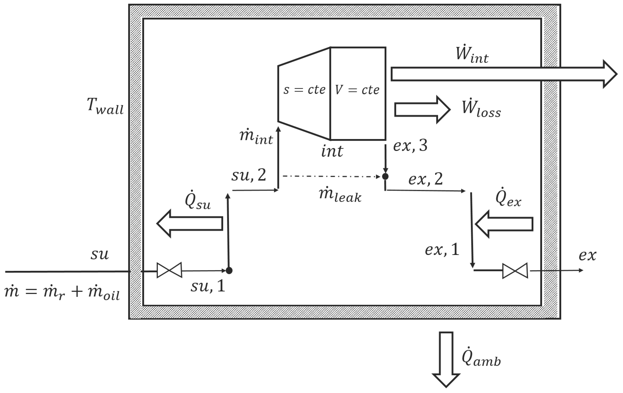
The modeling scheme considers a steady-state, counter-flow, moving boundary method which has been generalized to account for any phase condition for either side, namely hot side and cold side. The main inputs of the model are the PHEX geometry (number of plates, dimensions of the plate, wave length, amplitude of corrugation and Chevron angle, thermal conductivity of the plate) and the mass flow rate and inlet conditions of both streams in terms of pressure and enthalpy. A degree of freedom consists of the possibility to assign an extra channel to the hot or cold stream in the case of an even number of plates, i.e., odd number of channels. In fact, in a PHEX with N plates, there are $N-1$ total channels, which results in $N-2$ active counterflow sections, as shown in Figure 2a. The details of the calculation of the PHEX surface area can be found in [33]. The moving boundary heat exchanger model is characterized by its use of separate zones, the boundaries of which are defined by the thermodynamic phase change points of each fluid. The most general case where both fluids enter with single-phase states, undergo a complete phase change, and exit with single-phase states is shown schematically in Figure 2. The heat exchange rate with the surroundings is neglected in the current version of the model.

The physical bounds of the total heat transfer rate are obtained based on a pinch point analysis. Only phase-change pinch points are considered in the moving boundary model and only sub-critical conditions are allowed. The maximum physical heat transfer rate, ${\dot{Q}}_{max}$, is first assumed to be given by:

$${\dot{Q}}_{max}=min\left(\begin{array}{c}{\dot{m}}_c\left(h_c\left(T_{h,in},p_{c,in}\right)-h_c\left(T_{c,in},p_{c,in}\right)\right),\\ {\dot{m}}_h\left(h_h\left(T_{h,in},p_{h,in}\right)-h_h\left(T_{c,in},p_{h,in}\right)\right)\end{array}\right)$$

(7)

Once ${\dot{Q}}_{max}$ is evaluated, a list of enthalpies at the inlet, exit, and zone boundaries (if any) of each working fluid is constructed. Where a phase boundary is found for one fluid, the corresponding state in the other fluid is determined using an energy balance. Pinch point violations are checked and handled, as described in [32].

For a given heat transfer rate and inputs, the number of zones and phase boundaries can be directly determined. The ability of the code to correctly handle any phase configuration is useful for ORC systems. An extension to the code proposed in [32] has been added to handle incompressible fluids, such as thermal oils and lubricant oils where only the liquid phase is allowed.

For each zone, the surface area required to achieve the heat transfer rate defined by the zone boundaries is determined. The required heat conductance for the zone, $U{A}_{req}$, is calculated by applying the log mean temperature difference (LMTD) method. The use of the LMTD method, rather than the effectiveness-NTU method, made the code more concise and still able to handle two-phase conditions for pure fluids or mixtures.

The required heat conductance for a zone is defined by:

$$U{A}_{req}=\frac{{\dot{Q}}_{zone}}{\Delta T_{LMTD}}$$

(8)

Zero division errors that may occur while evaluating the LMTD function in Equation (8) have been avoided by introducing numerical tolerances. The heat transfer area fraction of the heat exchanger associated with the required heat conductance can be calculated. Noting that for heat exchangers with constant cross-section along their length, such as PHEX, the heat transfer area fraction reduces to a length fraction defined by:

$$w_{zone}=\frac{L_{zone}}{L}=U{A}_{req}\left(\frac{1}{h_{c,zone}{L}_{p}P}+\frac{t_w}{k_w{L}_{p}P}+\frac{1}{h_{h,zone}{L}_{p}P}\right)$$

(9)

where $L_p$ is the center-to-center distance between the ports of a plate and P is a constant dimension of the surface perpendicular to the direction of the heat transfer. A bounded solver is used to iterate on the heat transfer rate until the sum of length fractions in each zone is equal to unity, indicating that the entire surface area of the heat exchanger was utilized. In particular, the convergence is attained by driving to zero the following residual function:

$$residual\left(\dot{Q}\right)=1-\sum _{zone}{w}_{zone}$$

(10)

The bounded solver used in the current version of the model is based on Brent’s method. The brentq function available in the scipy.optimize module for the Python programming language has been employed in the code.

Due to the fact that the moving boundary model presented is general, the same code can be used to simulate the evaporator, condenser and regenerator. Proper heat transfer correlations for evaporating and condensing streams have been implemented. For instance, the Cooper pool boiling correlation is used to find the heat transfer coefficient for evaporating flow [35]. To allow for the possibility of evaporating flow at high quality, the Shah chart correlation for boiling heat transfer has also been included and it can be chosen optionally by the user [36]. The heat transfer coefficient correlation for condensing flow used in the model refers to the study conducted by Longo on condensing refrigerant flow in PHEX [37]. Note that no general two-phase heat transfer correlations have been implemented for two-component mixtures. The pressure drops of each fluid are calculated by assuming an appropriate pressure drop correlation for each zone. In the solution scheme, the pressure drops are not included in the heat transfer calculations but they are calculated independently. This makes the model solution more straightforward by eliminating the need to iterate between pressure drop and heat transfer in each zone. Additional documentation can be found in [33].

The PHEX moving boundary model allows the estimation of the refrigerant charge in the heat exchanger. Due to the fact that during the operation of an ORC, charge fluctuations occur in the PHEX, a detailed model to estimate the charge in each zone has been developed. In particular, the total working fluid charge in a PHEX is given by:

$${\mathit{Charge}}_{PHEX}=\sum _{zone}{\mathit{Charge}}_{zone}=\sum _{zone}{V}_{PHEX}{w}_{zone}{\overline{\rho }}_{zone}$$

(11)

where $V_{PHEX}$ is the combined volume of all channels for either the primary or secondary fluid side, $V_{PHEX}{w}_{zone}$ represents the volume of a single zone and ${\overline{\rho }}_{zone}$ is the average fluid density of the zone. In the case of single-phase zone, ${\overline{\rho }}_{zone}$ is calculated assuming an average temperature between inlet and outlet of the zone. For two-phase zones, ${\overline{\rho }}_{zone}$ is obtained by weighting the density of the liquid phase and vapor phase with an average void fraction for the considered zone. Mathematically, this can be expressed as:

$${\overline{\rho }}_{zone}={\overline{\alpha }}_{zone}{\rho }_v+\left(1-{\overline{\alpha }}_{zone}\right){\rho }_l$$

(12)

where the average void fraction over the length of the zone is given by:

$${\overline{\alpha }}_{zone}=\frac{1}{x_{out}-x_{in}}{\int }_{x_{in}}^{x_{out}}\frac{1}{1+S_{Zivi}\frac{{\rho }_v}{{\rho }_l}\frac{1-x}{x}}dx$$

(13)

where $S_{Zivi}$ is the slip model defined by Zivi [38]. The main inaccuracies of this charge model may lie on the void fraction model used to estimate the density in the two-phase zone, where inaccuracies may occur. An improvement to this model proposed in this paper would be to implement different void fraction models to account for different flow patterns [38]. Another source of error is that a quality-averaged void fraction is used rather than a length-averaged void fraction. This is done for convenience to avoid estimating the quality variation along the length of the heat exchanger, but it does not necessary represent the distribution of voids within the zone.

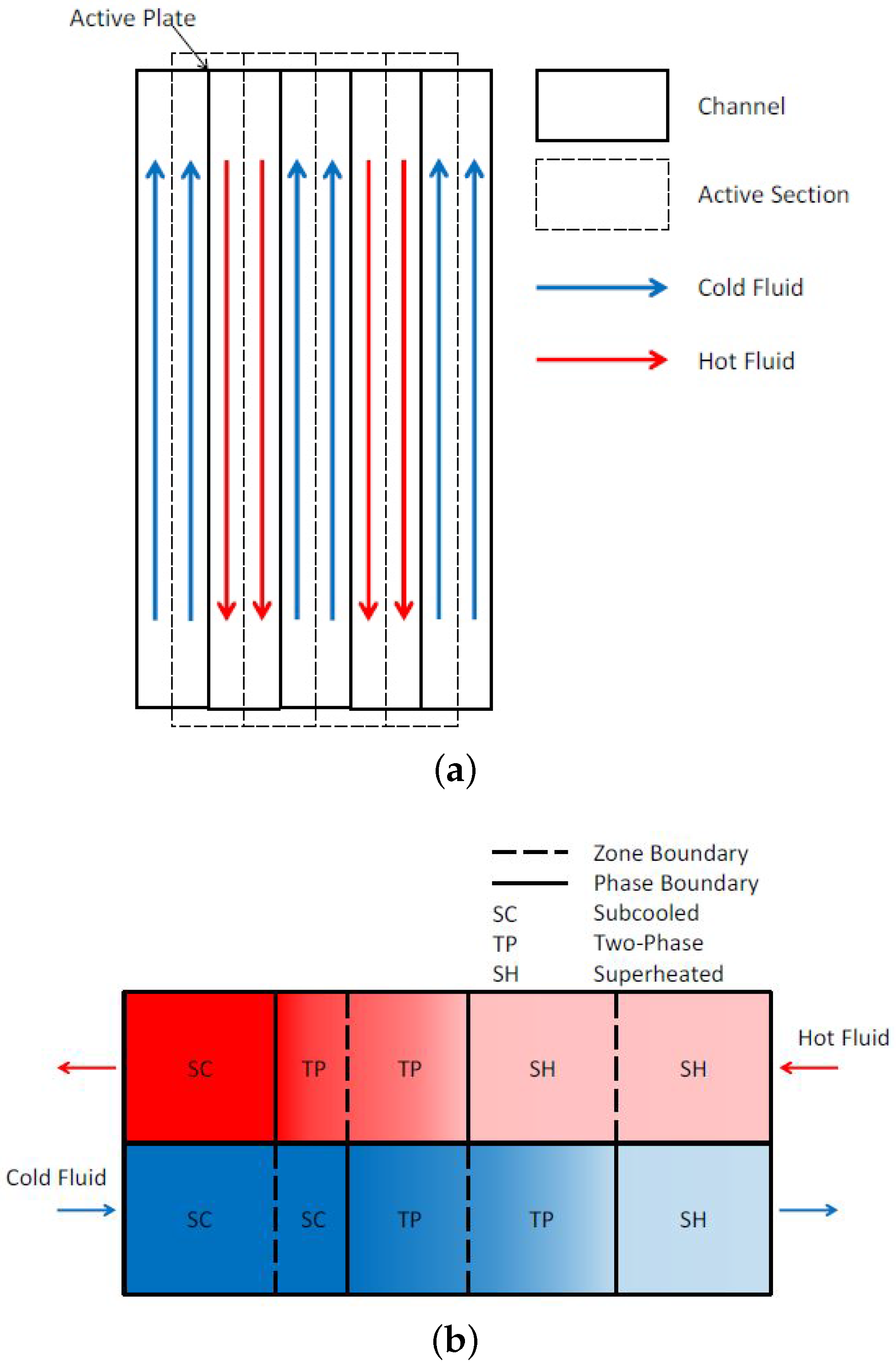
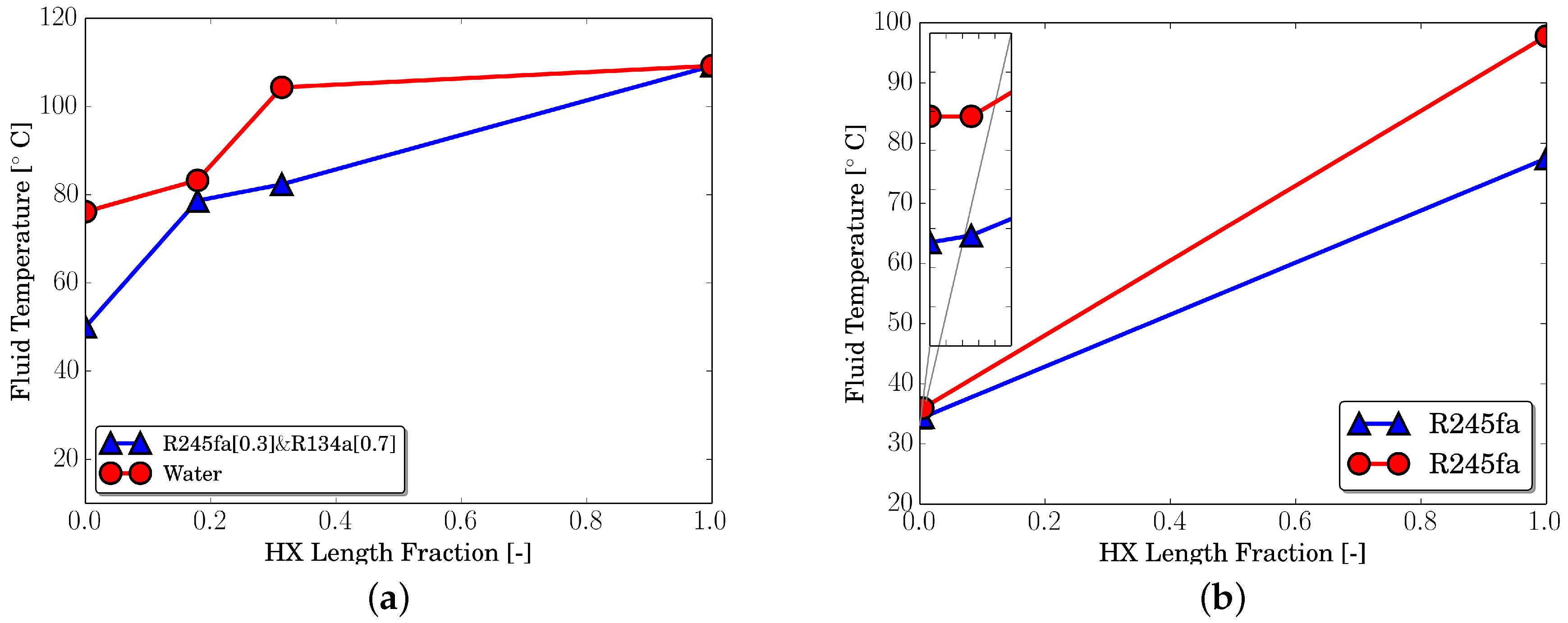
Examples of temperature profiles across the PHEX (both as condenser and as evaporator) are shown in Figure 3. The fluid combinations are representative of the two ORC installations considered in Section 4. The PHEX model allows us to make use of the extended incompressible fluid library available in CoolProp [26]. Three examples are proposed: a condenser with a mixture of ethylene glycol and water as cooling medium, Figure 3b, an evaporator using a thermal oil (Therminol 66) as hot source, Figure 3c, a lubricant oil heater, Figure 3e. An example of heat transfer between a zeotropic mixture of R134a and R245fa and hot water is presented in Figure 4a. Phase-change conditions are also allowed in both streams. In ORC systems, this situation may occur at the regenerator, as shown in Figure 4b.

2.3. Pump Models

The pump models implemented are based on empirical maps. A distinction is made between volumetric and centrifugal pumps. Due to the fact that volumetric and centrifugal pumps have different characteristic curves, appropriate empirical correlations are selected to better capture their behaviors. In both cases, two empirical correlations have been used. One models either the volumetric or mass flow rate, and another correlation gives the performance of the pump, either the input power or the pump efficiency.

For the volumetric pump two sets of correlations are considered:

(i)

mass flow rate and input electric power;

(ii)

normalized volumetric flow rate and pump efficiency.

In the case of the centrifugal pump, only one model has been implemented:

(i)

mass flow rate and pump efficiency with normalized input values.

The different models for each pump type are listed for compactness and clearness in

Table 1. Pump models available.

Type of Pump	Correlations
Volumetric	${\dot{m}}_{p,calc}=a{N}_p+b$
	$\begin{array}{cc}\hfill {\dot{W}}_p& ={\dot{W}}_{p,ref}\left(w_1\frac{N_p}{N_{p,ref}}+w_1\right)\hfill \\ \hfill {\dot{W}}_{p,ref}& =c\Delta p_p+d{|}_{\begin{array}{c}{N}_p=N_{p,ref}\end{array}}\hfill \end{array}$
	${\dot{V}}_p^{*}=a{N}_p^{*}+b\Delta p_p^{*}+c{N}_p^{*}\Delta p_p^{*}+d$
	$\begin{array}{c}{\eta }_p=a_1{e}^{a_2{N}_p^{*}}+a_3{e}^{a_4{\left(v_{su,p,wf}\Delta p_p\right)}^{*}}+a_5{e}^{a_6{N}_p^{*}+a_7{\left(v_{su,p,wf}\Delta p_p\right)}^{*}}+a_8\\ with{X}^{*}=X/X_{ref}\end{array}$
Centrifugal	${\dot{V}}_p=c_1+c_2\Delta p_p+c_3\Delta p_p^2+c_4{f}_p+c_5{f}_p^2$
	$\begin{array}{cc}\hfill {\eta }_{oa,p}& =\sum _{i=1}^{n=3}{c}_i{\left(\Delta p_p^{*}\right)}^i+\sum _{i=1}^{n=3}{c}_i{\left(f_p^{*}\right)}^i+\sum _{i=1}^{n=3}{c}_i{\left(r_{p,p}^{*}\right)}^i+\sum _{i=1}^{n=3}{c}_i{\left({\rho }_p^{*}\right)}^i\hfill \\ & +\sum _{i=1}^{n=2}{X}^i{|}_{\begin{array}{c}X=r_{p,p}^{*},f_p^{*},{\rho }_p^{*}\end{array}}\left[\Delta p_p^{*}+{\left(\Delta p_p^{*}\right)}^2\right]+\sum _{i=1}^{n=2}{X}^i{|}_{\begin{array}{c}X=r_{p,p}^{*},{\rho }_p^{*}\end{array}}\left[f_p^{*}+{\left(f_p^{*}\right)}^2\right]\hfill \\ & +\sum _{i=1}^{n=2}{\left({\rho }_p^{*}\right)}^i\left[r_p^{*}+{\left(r_p^{*}\right)}^2\right]\hfill \end{array}$
	with $Y^{*}=\frac{Y-Y_{ref}}{Y_{ref}}$

. The typical volumetric pump curve is characterized by a linear relationship between the volumetric flow rate, ${\dot{V}}_p$ and the rotational speed, $N_p$ for different discharge pressures, $p_{ex,p}$. A linear correlation can be obtained to express the volumetric flow rate of the pump as a function of the rotational speed and discharge pressure:

$$\begin{array}{cc}\hfill {\dot{V}}_p& =slope·N_p+intercept\hfill \\ & =\left[N_{p,max}-\frac{p_{ex,p}-p_{ex,p,min}}{p_{ex,p,max}-p_{ex,p,min}}\left(N_{p,max}-N_{p,min}\right)\right]\left(N_p-N_{p,min}\right)+{\dot{V}}_{p,min}\hfill \end{array}$$

(14)

where $N_{p,min}$, $N_{p,max}$, $p_{ex,p,min}$ and $p_{ex,p,max}$ are known from the pump manufacturer curves. From Equation (14), simplified empirical correlation can be derived and coefficients can be fit to available experimental data. By considering the mass flow rate rather than the volumetric flow rate, Equation (14) can be rewritten as:

$${\dot{m}}_{p,calc}=a\left(p_{ex,p}\right)N_p+b$$

(15)

where the parameters a and b are obtained by minimizing an objective function. By introducing a set of fitting parameters, $a_1$, $b_1$, $c_1$ and $d_1$, and by normalizing the input and output values with respect to a set of reference values to improve the robustness of the regression, an equivalent form of Equation (14) can be obtained:

$${\dot{V}}_p^{*}=a_1{N}_p^{*}+b_1\Delta p_p^{*}+c_1{N}_p^{*}\Delta p_p^{*}+d_1$$

(16)

where the discharge pressure $p_{ex,p}$ in Equation (14) has been substituted by the pressure difference across the pump, $\Delta p_p$, due to a better agreement with the experimental data. The centrifugal pump curves are well represented by second-order polynomial functions. By choosing the pressure increase provided by the pump, $\Delta p_p$ and its frequency, $f_p$, as input variables, the volumetric flow rate can be expressed as,

$${\dot{V}}_p=c_1+c_2\Delta p_p+c_3\Delta p_p^2+c_4{f}_p+c_5{f}_p^2$$

(17)

where the coefficients $c_1,...,c_5$ are obtained by regression.

The input power of the pump, ${\dot{W}}_p$, is calculated as the ratio of the reversible work rate, ${\dot{W}}_{is,p}$, to the pump efficiency, ${\eta }_p$. A choice can be made whether using an empirical correlation for the input power or the pump efficiency and to calculate the other term. In the case of the volumetric pump both correlations have been developed. By defining the reference power of the pump, ${\dot{W}}_{p,ref}$, as a linear function of the pump pressure difference at the chosen reference rotational speed, $N_{p,ref}$, the pump power at any rotational speed can be calculated as:

$${\dot{W}}_p={\dot{W}}_{p,ref}\left(w_1\frac{N_p}{N_{p,ref}}+w_2\right)$$

(18)

A correlation for the pump isentropic efficiency can be used instead of the pump power because it provides better physical constraints on the model and it guarantees that the Second Law of Thermodynamics is not violated. Analogously to the pump power equation, the pump efficiency can be related to a reference pump efficiency, ${\eta }_{p,ref}$ at a chosen rotational speed. From experimental data, an exponential decay of the pump efficiency with the pump speed was observed. The functional form is given by

$$\frac{{\eta }_p}{{\eta }_{p,ref}}=D{e}^{E\frac{N_p}{N_{p,ref}}}+F$$

(19)

where the reference pump efficiency is a function of the mass-specific reversible work of the pump, $v_{su,p,wf}\Delta p_p$ at the reference pump speed, and the coefficients $D,E,F$ are determined empirically. Mathematically:

$${\eta }_{p,ref}=A{e}^{B\left(v_{su,p,wf}\Delta p_p\right)}+C$$

(20)

By introducing Equation (20) in Equation (19) and by normalizing the input values with respect to the reference conditions, the final form of the correlation for the pump efficiency can be obtained, as listed in Table 1. A similar approach has been considered for the centrifugal pump. The pump efficiency has been correlated to different non-dimensional terms normalized with respect reference values. Due to the fact that experimental data of the pump isentropic efficiency did not show a clear trend with respect to the mass flow rate, rotational speed and pump pressure difference, a third-order polynomial function with several cross-terms has been selected. The pump isentropic efficiency has been expressed in terms of the pressure difference, pressure ratio, density of the working fluid and frequency. The functional form can be written as:

$${\eta }_{p,centr}=f\left(\Delta p_p^{*},r_{p,p}^{*},{\rho }_{wf}^{*},f_p^{*},\right)$$

(21)

where $\Delta p_p=p_{ex,p}-p_{su,p}$ and $r_{p,p}=p_{ex,p}/p_{su,p}$. The complete formulation can be found in Table 1.

2.4. Expander Models

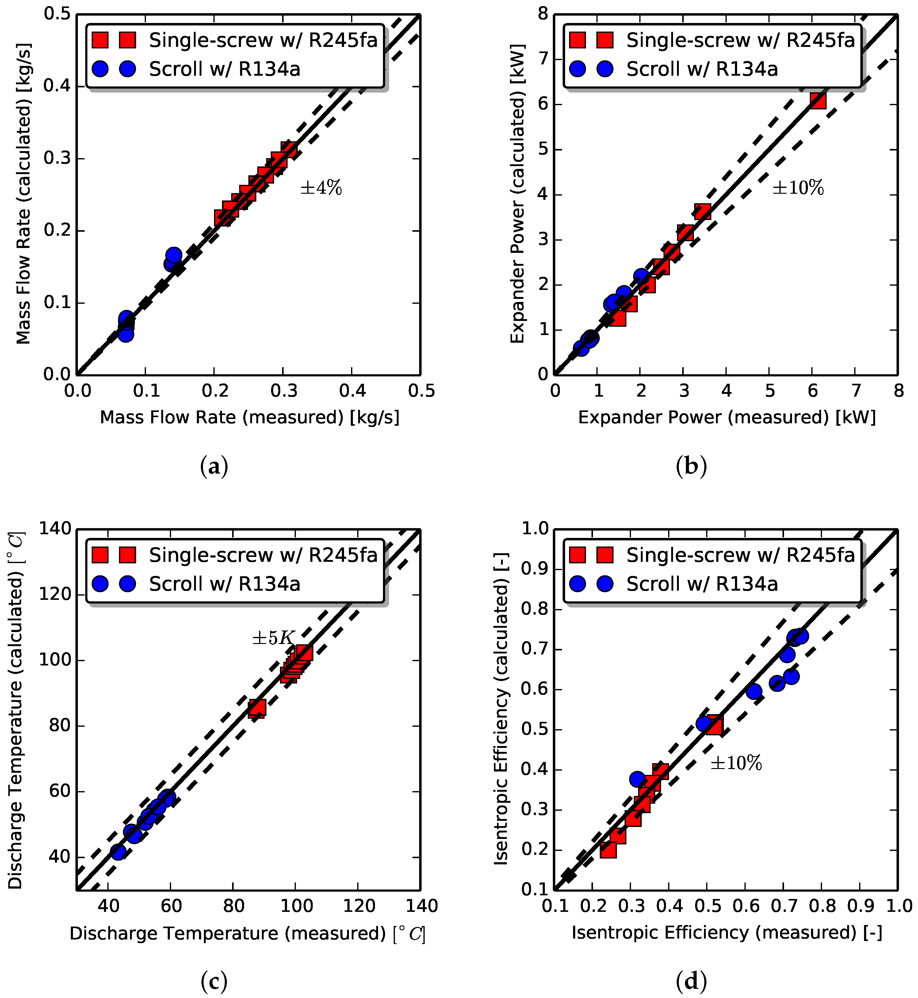
In this study, positive displacement expanders are considered as suitable devices for low-grade heat recovery [6]. The expander has been modeled using an empirical map and also by means of a semi-empirical model.

Empirical model. The performance of a volumetric expander is well characterized by the filling factor and the isentropic efficiency. Two empirical correlations can be developed to account for different operating conditions of the expander. The filling factor along with the displacement rate of the machine is used to calculate the mass flow rate for a given inlet state conditions and working fluid. It is defined as:

$${\mathrm{\Phi }}_{FF}=\frac{{\dot{m}}_r{v}_r\left(T_{exp,su},p_{exp,su}\right)}{V_{D,exp}\frac{N_{exp}}{60}}$$

(22)

where $V_{D,exp}$ is the displacement volume of the expander. An empirical correlation similar to the one proposed by Declaye et al. [39] is employed. Its expression is given as:

$${\mathrm{\Phi }}_{FF}=k_1+k_{2}ln{\left(N_{exp}\right)}^{*}+k_3{\left(\frac{p_{ex}}{p_{su}}\right)}^{*}+k_4{p}_{su}^{*}$$

(23)

where $k_1,..,k_4$ are the fitting parameters to be obtained by regression. Note that the filling factor is a function of the inlet pressure, the pressure ratio and the rotational speed which have been normalized by a set of reference values as follows:

$$\begin{array}{c}\hfill N_{exp}^{*}=\frac{N_{exp}}{N_{exp,ref}}\\ \hfill {\left(\frac{p_{ex}}{p_{su}}\right)}^{*}=\frac{\left(\frac{p_{ex}}{p_{su}}\right)-{\left(\frac{p_{ex}}{p_{su}}\right)}_{ref}}{{\left(\frac{p_{ex}}{p_{su}}\right)}_{ref}}\\ \hfill p_{su}^{*}=\frac{p_{su}-p_{su,ref}}{p_{su,ref}}\end{array}$$

(24)

A second empirical relationship is used to model the expander isentropic efficiency. By doing so, the expander power output can be obtained by calculating the mass flow rate from Equation (22) and the mass-specific isentropic work for a given expender inlet temperature and pressure ratio. As first proposed by Declaye et al. [39], Pacejka’s equation is suitable to represent the behavior of a volumetric expander isentropic efficiency with respect to either the volume ratio or pressure ratio at different rotational speeds. Pacejka’s equation has been applied to scroll expanders [39,40] as well as to a single-screw expander [22] with high accuracy in the prediction of the isentropic efficiency. This shows the versatility of the equation as a modeling tool for different types of volumetric expanders. The original equation described by Pacejka and Bakker [41] is expressed by:

$$\begin{array}{c}\hfill y=Dsin\left\{C{tan}^{-1}\left[Bx-E\left(Bx-{tan}^{-1}\left(Bx\right)\right)\right]\right\}\\ \hfill E=\frac{B{x}_{max}-tan\left(\frac{\pi }{2C}\right)}{B{x}_{max}-{tan}^{-1}\left(B{x}_{max}\right)}\end{array}$$

(25)

where y and x indicate a position on the ordinate and abscissa, respectively. Physical values related to the expander operating conditions are selected for the abscissa and ordinate axes to represent the expander isentropic efficiency. Furthermore, functional forms are required for the coefficients appearing in Equation (25). A more in-depth description of the equation and its parameters can be found in [34,39].

Semi-empirical model. A semi-empirical model has a computational time comparable to an empirical model while retaining physically meaningful parameters that can be identified from experimental data. The typical increase in robustness due to less modeling detail involved and the absence of differential equations makes the semi-empirical model suitable to be included in an overall cycle model. The semi-empirical model described here is an extension to the well-known semi-empirical model initially developed by Winandy et al. [42] and then successfully applied to scroll expanders by Lemort et al. [43] and Quoilin et al. [1]. Such a model has been demonstrated to be applicable to different types of volumetric expanders, e.g., scroll, screw and piston types, by Guillaume et al. [9]. The expander model is modified to take into account the presence of oil in the machine throughout the expansion process. In the following, the major changes related to two-phase pressure drops, leakage and the actual expansion compared to the original model are only briefly described. A more comprehensive description can be found in [40,44].

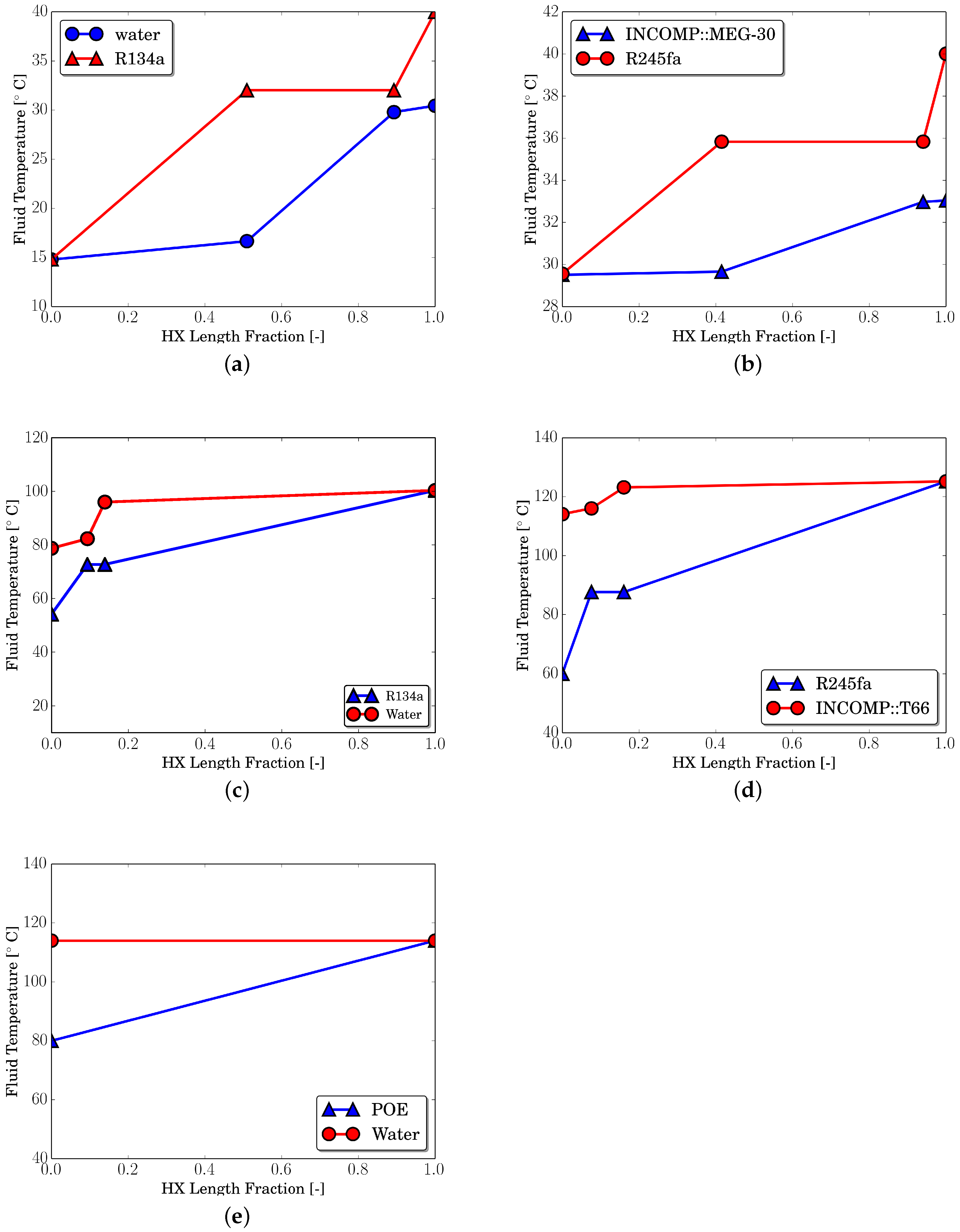
The evolution of the working fluid and lubricant oil through the expander is decomposed in several steps, as shown in Figure 5:

• adiabatic supply pressure drop;
• isobaric supply cooling;
• fictitious internal leakage;
• adiabatic reversible expansion to the internal pressure ratio imposed by the built-in volume ratio of the expander;
• adiabatic expansion at a constant volume;
• adiabatic mixing between the flow exiting the expansion chamber and the internal leakage flow;
• isobaric exhaust heat transfer;
• adiabatic discharge pressure drop.

The working fluid and lubricant oil are considered to be in thermal and mechanical equilibrium so that a homogeneous mixture model can be applied. The total mass flow rate entering the expander is given by

$${\dot{m}}_{exp}={\dot{m}}_r+{\dot{m}}_{oil}=\left(1+y_{oil}\right){\dot{m}}_r$$

(26)

where $y_{oil}$ represents the ratio between the oil mass flow rate to the working fluid mass flow rate. The pressure drop through the suction port of the expander is modeled by calculating the mass flow rate of a compressible gas-liquid mixture through a nozzle. Based on the Chisholm [38] model, such a mass flow rate can be calculated by imposing the conservation of momentum between upstream and downstream conditions of the orifice as:

$$\dot{m}=C_d{A}_{eff}{\left(2{\int }_{p_{down}}^{p_{up}}{v}_{eff}dp\right)}^{0.5}{\left(v_{eff,down}^2-{\sigma }^2{v}_{eff,up}^2\right)}^{-0.5}$$

(27)

where $C_d$ represents the two-phase flow coefficient calculated according to Morris [45], the effective specific volume or momentum specific volume $v_e$ is calculated by assuming the case of a separated-phase flow with some liquid entrainment in the gas phase and flowing at the same velocity. The correlation of $v_e$ and the associated effective slip ratio between the phases can be found in [38,45]. The coefficient ${\sigma }^2$ is the throat to upstream area ratio of a flow path, which can be approximated to be zero if the throat area is treated as being infinitely smaller than of the upstream area. Under this assumption, the lowest flow rate possible with this model is computed [29].

Dealing with two-phase leakage flows leads to complex fluid dynamic effects. In order to take into account the presence of oil in the leakage paths without increasing the computational effort of the model, the total leakage area has been corrected by a factor proportional to the oil ratio that enters the machine. In other words, the more the oil fraction is increased, the more the working fluid leakage is reduced, which is indeed one of the purposes of the lubricant oil. Mathematically, this statement is expressed by still considering a compressible flow of working fluid through a nozzle where the throat area, $A_{r,leak}$, is a parameter to be determined empirically:

$$A_{r,leak}=A_{tot,leak}-A_{oil,leak}=A_{tot,leak}-y_{oil}{A}_{r,leak}\frac{v_{oil,up}}{v_{r,thr,leak}}$$

(28)

The working fluid leakage flow rate is given by:

$${\dot{m}}_{r,leak}=C_{r,thr,leak}\frac{A_{r,leak}}{v_{r,thr,leak}}$$

(29)

Therefore, the internal refrigerant mass flow rate that contributes to generate positive work is given by:

$${\dot{m}}_{r,int}={\dot{m}}_r-{\dot{m}}_{r,leak}$$

(30)

and the new oil fraction entering the expansion chamber is defined as:

$$x_{oil}=y_{oil}\frac{{\dot{m}}_r}{{\dot{m}}_{r,int}}$$

(31)

The expansion process is divided into two steps as shown in the original model [1,43]. At first, the oil-refrigerant mixture undergoes an isentropic expansion where the specific entropy of the mixture defined as $s_{mix,int}=s_{r,int}+x_{oil}{s}_{oil,int}$ is kept constant. The internal isentropic specific-work is given by:

$$w_{int,is}=h_{r,su2}-h_{r,int}+x_{oil}\left(h_{oil,su2}-h_{oil,int}\right)$$

(32)

Due to the presence of oil, the built-in volume ratio becomes an effective built-in volume ratio:

$$r_{v,int}^{*}=\frac{v_{r,int}}{v_{r,su2}}$$

(33)

The second step is an expansion at constant machine volume. The work associated with this second step is expressed by:

$$w_{int,V}=\left(p_{r,int}-p_{r,ex2}\right)\left(v_{r,int}+x_{oil}{v}_{oil,su2}\right)$$

(34)

where implicitly it is assumed that $p_r=p_{oil}$. Finally, the overall isentropic efficiency of the expander is given by:

$${\eta }_{exp,is}=\frac{{\dot{m}}_{r,int}\left(w_{int,is}+w_{int,V}\right)-{\dot{W}}_{loss}}{{\dot{m}}_r\left[h_{r,su}-h_{r,ex,is}+y_{oil}\left(h_{oil,su}-h_{oil,ex,is}\right)\right]}$$

(35)

where ${\dot{W}}_{loss}$ accounts for the visco-mechanical losses in the expander. The visco-mechanical losses are assumed to have a linear dependency with the rotational speed and the oil fraction. A constant frictional torque, ${\tau }_{loss}$, is introduced in the model along with a viscous torque due to the presence of lubricant oil. The viscous torque is given by:

$${\tau }_{{\mu }_{oil}}=C_{oil}{\mu }_{oil}\left(2\pi \frac{N_{exp}}{60}\right)$$

(36)

where $C_{oil}{\mu }_{oil}$ represents the viscous coefficient. Hence, the total losses are expressed as

$${\dot{W}}_{loss}={\dot{W}}_{loss,0}+2\pi \left({\tau }_{loss}+{\tau }_{{\mu }_{oil}}\right)\frac{N_{exp}}{60}$$

(37)

The semi-empirical model is closed by a shell energy balance over a fictitious wall envelope:

$${\dot{Q}}_{su}+{\dot{Q}}_{ex}+{\dot{W}}_{loss}-{\dot{Q}}_{amb}=0$$

(38)

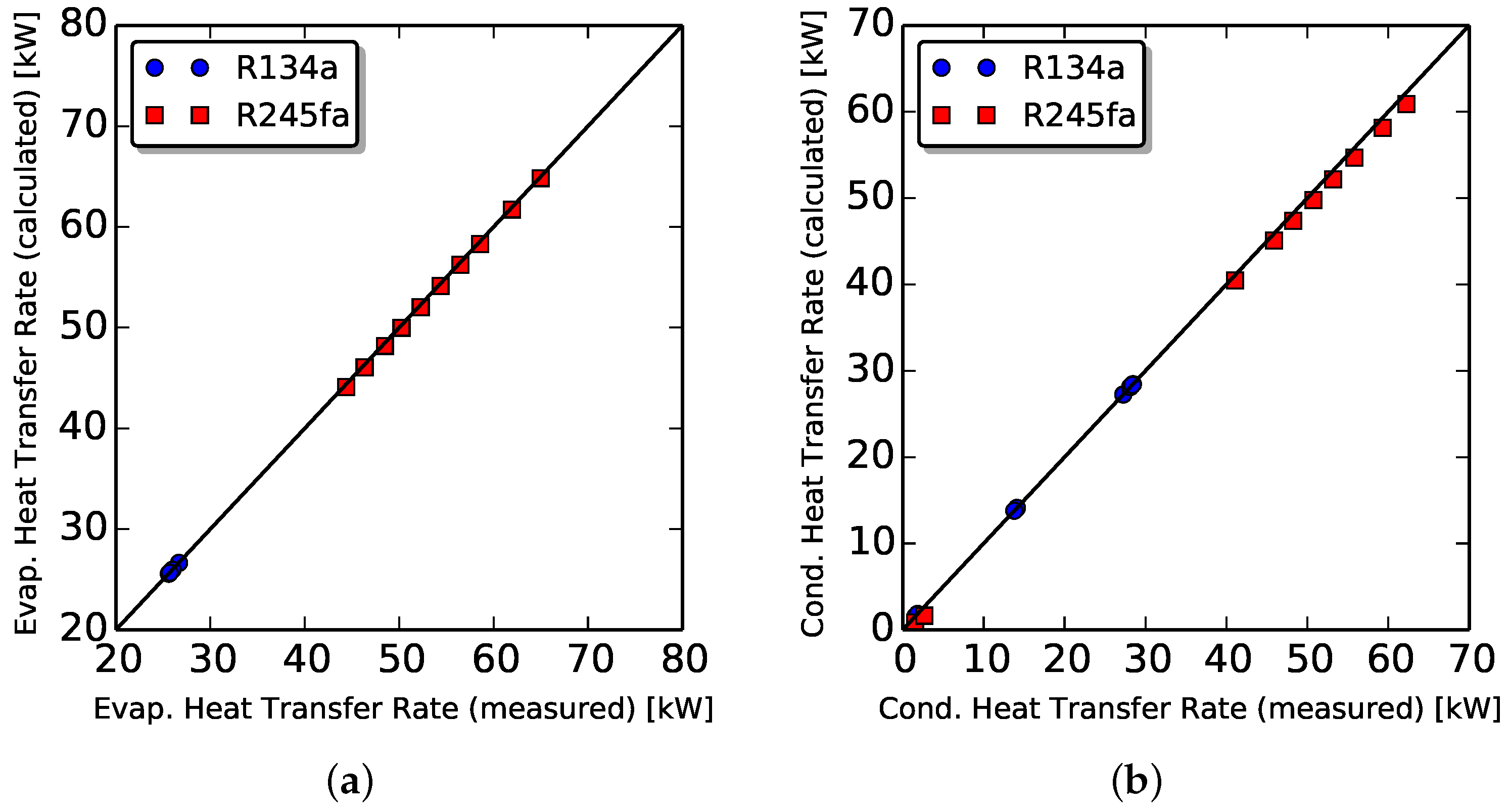
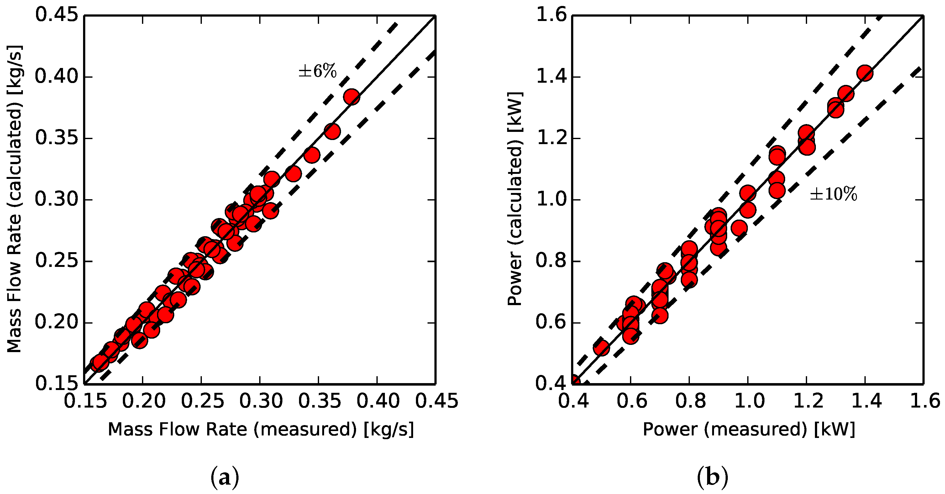
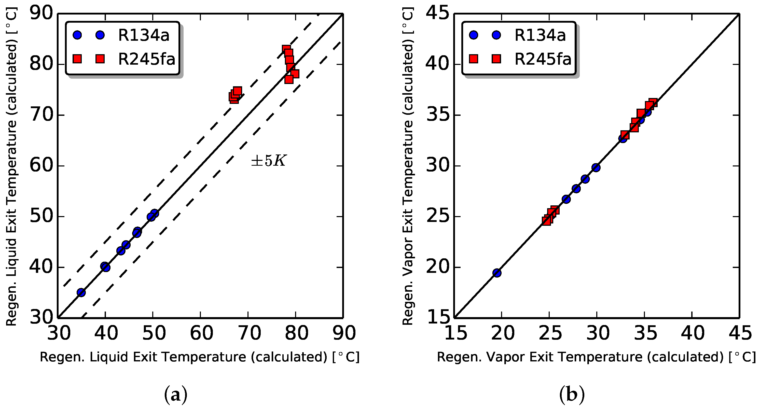
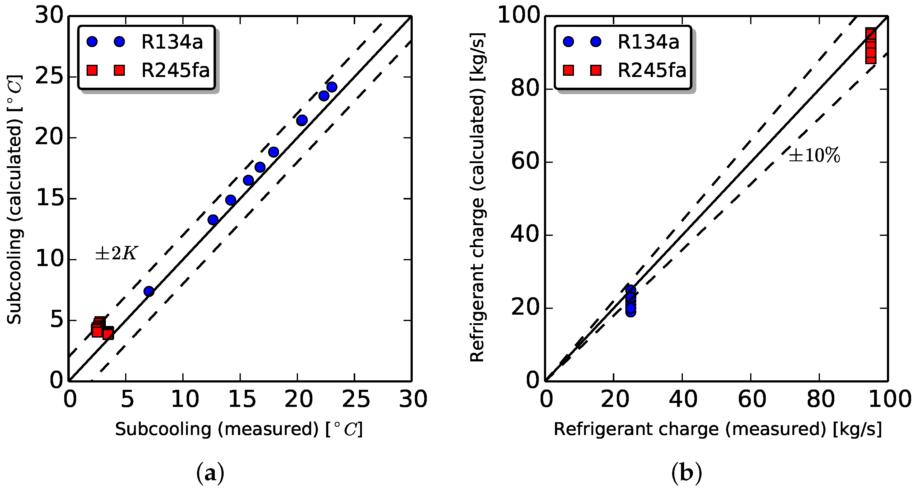
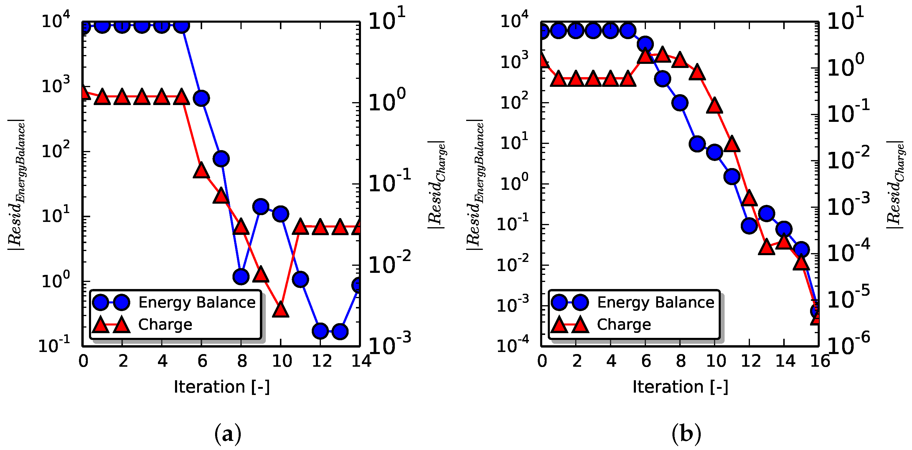
The semi-empirical model includes a set of fourteen parameters that have to be identified. A multi-parameter optimization is carried out by minimizing an objective function based on the errors on working fluid mass flow rate, the discharge temperature and the expander power output. These represents also the three main outputs of the model along with the expander isentropic efficiency. The objective function is defined as a weighted sum of the relative error between predicted and measured values for each of the variables considered:

$$\begin{array}{cc}\hfill obj\left({\dot{m}}_r,{\dot{W}}_{exp,sh},T_{exp,ex}\right)& =[\sum _i{\left(\frac{{\dot{m}}_{r,calc}-{\dot{m}}_{r,meas}}{{\dot{m}}_{r,meas}}\right)}^2+\frac{1}{\sqrt{2}}\sum _i{\left(\frac{{\dot{W}}_{r,sh,calc}-{\dot{W}}_{r,sh,meas}}{{\dot{W}}_{r,sh,meas}}\right)}^2\hfill \\ & +\sum _i{\left(\frac{T_{exp,ex,calc}-T_{exp,ex,meas}}{T_{exp,ex,meas,max}-T_{exp,ex,meas,min}}\right)}^2{]}^{1/2}\hfill \end{array}$$

(39)

The weighting factors are chosen to give each error term approximately the same weight. For the expander discharge temperature term, the weight factor can be expressed as the difference between the maximum and minimum discharge temperature values. However, in this work $1/\sqrt{30}$ has been selected for both expanders. A similar objective function was also used by Quoilin et al. [1].

2.5. Liquid Receiver Model

A steady-state model of a liquid receiver has been included in the cycle. It is well known that liquid receivers in ORC systems have a damping function, absorbing the mass flow rate fluctuations which may occur in transient operation. Additionally, the liquid receiver serves as a refrigerant charge buffer tank to help maintain the subcooling level at the condenser outlet at a minimum. Without a liquid receiver, adjustment of the subcooling level for a given operating point requires an adjustment of the working fluid charge of the system. The liquid receiver is considered to be adiabatic and its volume represents the only parameter to be specified (pressure drops at inlet/outlet are neglected). The steady-state level of the receiver is given by:

$$level=\left(\frac{h_{wf,v,sat}-h_{wf,su}}{h_{wf,v,sat}-h_{wf,l,sat}}\right)\frac{{\rho }_{r,su}}{{\rho }_{l,sat}}=\frac{m_{wf,l,sat}{v}_{wf,l,sat}}{m_{wf,tot}{v}_{wf,su}}=\frac{V_l}{V_{tot}}=\frac{V_l}{{(ID/2)}^2{H}_{eff}}$$

(40)

where $ID$ and $H_{eff}$ represent the internal diameter and the effective height of the liquid receiver, respectively. The volume of the liquid receiver is used to estimate the refrigerant charge.

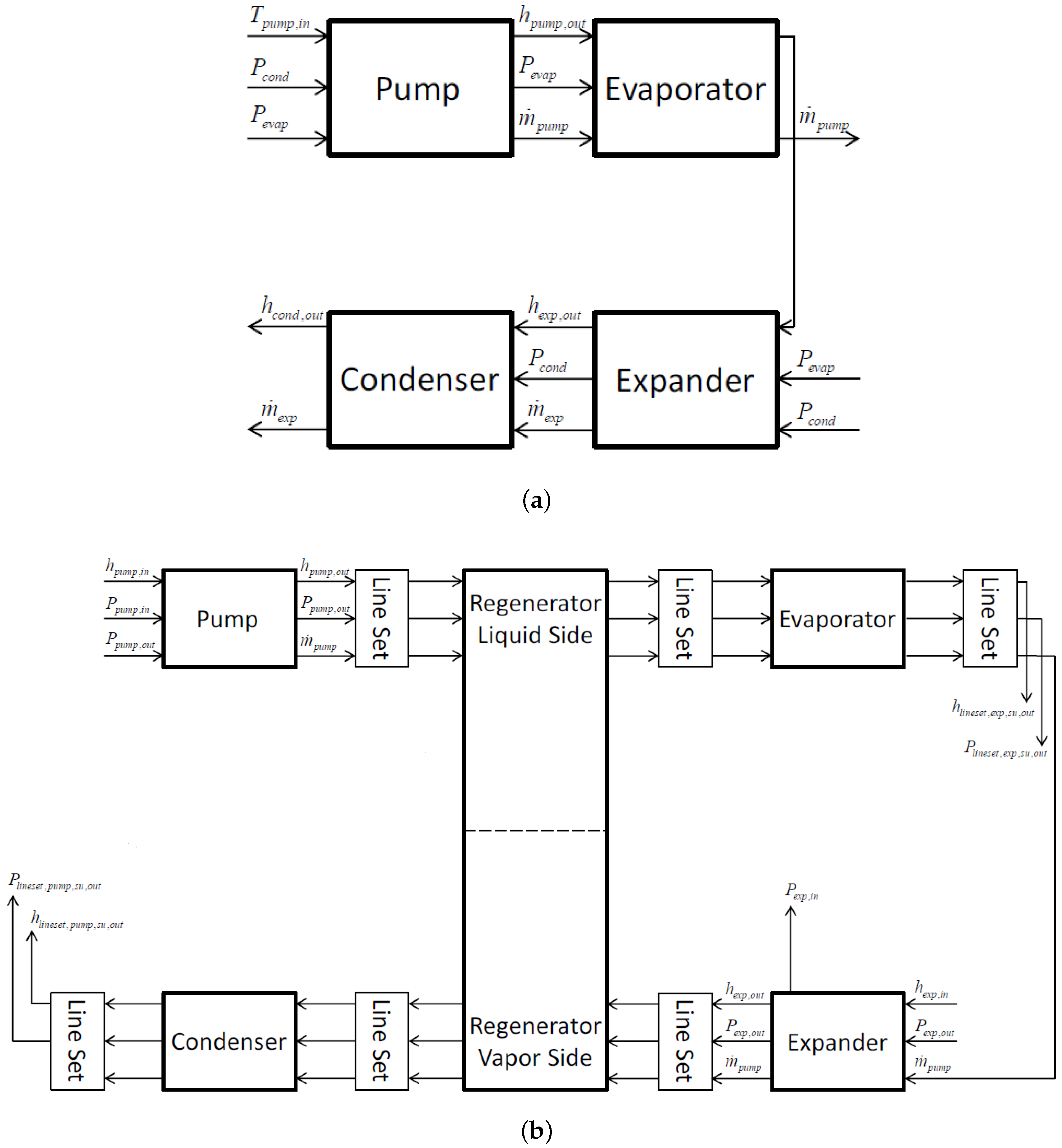
2.6. Line Set Model

The line sets of the ORC system carrying the working fluid are considered in the overall cycle model. The main reasons to consider the line sets are to determine the pressure drop between the main cycle components and to give a more accurate estimation of the charge of the working fluid. The following line sets are included in cycle model:

• liquid receiver exit to pump inlet;
• pump exit to liquid side of the regenerator;
• regenerator liquid side exit to evaporator inlet;
• evaporator exit to expander inlet;
• expander exit to vapor side of the regenerator;
• regenerator vapor side exit to condenser inlet;
• condenser exit to liquid receiver inlet.

Each line set is modeled as an equivalent tube with inner and outer diameters (ID and OD). The equivalent length of each section ($ID=const$) of the line set includes straight sections, tees, elbows and other fittings. It is calculated using the method and loss coefficients of Munson et al. [46]. In the calculation of the pressure drops, a distinction is made to account for single and two-phase flow conditions, as proposed by Woodland [34]. In the case of single-phase flow, the Darcy friction factor is used and the pressure drop for a certain ID is given by:

$$\Delta p_{lineset}{|}_{\begin{array}{c}ID=const\end{array}}=f\frac{\sum L_{straight}+\sum L_{eq,fitting}}{ID}\frac{\rho v^2}{2}$$

(41)

If two-phase flow conditions occur, the original form of the Lockhart-Martinelli method for two-phase frictional pressure drop in tubes [47] is used. The equivalent lengths of the fittings are computed using Churchill’s correlation for the friction factor under the hypothesis of liquid-only. The pressure drop of each section of the lineset is then given by the product of the Lockhart-Martinelli pressure gradient and the total equivalent length of the lineset:

$$\Delta p_{lineset}{|}_{\begin{array}{c}ID=const\end{array}}=-{\left(\frac{dp}{dz}\right)}_F\left(\sum L_{straight}+\sum L_{eq,fitting}\right)$$

(42)

The total pressure drop of a certain lineset is given by the sum of each section’s pressure drop.

The lineset model includes also a simplified model for the heat losses. The overall heat transfer coefficient of the lineset, $U{A}_{lineset}$, is the sum of the thermal resistance of the tube, the thermal resistance associated with the insulation and the convective $UA$ values associated with the inside and outside of the tube:

$$U{A}_{lineset}={\left(\frac{1}{U{A}_{ID}}+\frac{1}{U{A}_{0D}}+R_{lineset}+R_{insulation}\right)}^{-1}$$

(43)

If heat losses exist in a lineset with two-phase flow, then the pressure gradient in Equation (42) represents an average pressure gradient along the lineset flow direction.

The working fluid charge of the lineset is calculated analogously to the method applied to each zone of the heat exchanger. If a lineset is assumed to be adiabatic, then the average void fraction (Equation (13)) under two-phase flow conditions is equal to the void fraction at the inlet quality of the lineset.

2.7. Oil Separator

The oil separator separates the lubricant oil from the refrigerant as a primary function. As a secondary function, it serves as a buffer reservoir for the oil. In practice, zero solubility of the refrigerant in oil is not achievable. In fact, in the oil separator, the chemical equilibrium determines the amount of refrigerant that remains dissolved in the oil. Generally, the solubility mass fraction is a function of both pressure and temperature. Typically, it increases as the pressure increases for a given temperature and it decreases as the temperature increases for a given pressure. The effects of the working fluid solubility in the lubricant oil on the cycle performance could be further investigated.

The oil separator is modeled as adiabatic meaning the separation process is assumed to be isothermal and an energy balance is used to estimate the mass fraction of refrigerant dissolved in the oil, as proposed by Bell [29]. The mass balance over the oil separator is expressed by:

$$\underset{\text{Ref+Oil separator inlet}}{\underbrace{{\dot{m}}_r+{\dot{m}}_{oil}}}=\underset{\text{Pure Ref. Vapor}}{\underbrace{{\dot{m}}_{r,v}}}+\underset{\text{Oil + solved Ref.}}{\underbrace{{\dot{m}}_{oil}+x_{solved}{\dot{m}}_{oil}}}$$

(44)

The oil mass flow fraction leaving the separator is given by:

$$x_{oil,sep}=1-x_{r,solved}=1-\frac{{\dot{m}}_{r,solved}}{{\dot{m}}_{r,solved}+{\dot{m}}_{oil}}$$

(45)

3. Solution Scheme

The independent components are properly assembled to create the overall cycle model. A set of inputs is required to run the cycle and includes:

• the working fluid;
• hot and cold source fluid types;
• inlet state conditions and mass flow;
• pump and expander rotational speed;
• the expander swept volume.

The cycle model can be solved with respect to the subcooling or the total working fluid charge. Depending on the choice of the solver, the subcooling or the total charge must be specified as input. The list of inputs of the cycle model can be found in

Table 2. Required inputs to the overall ORC model.

Variable	Description
$PropertyWrapper$	Selection of CoolProp or Refprop
	to retrieve the thermophysical properties
Ref	Working fluid or mixture name as a string
Ref ${}_h$	Heat source fluid name as a string
$T_{h,in}$	Heat source fluid inlet temperature
$p_{h,in}$	Heat source fluid inlet pressure
${\dot{m}}_h$	Heat source fluid mass flow rate
Ref ${}_c$	Heat sink fluid name as a string
$T_{c,in}$	Heat sink fluid inlet temperature
$p_{c,in}$	Heat sink fluid inlet pressure
${\dot{m}}_c$	Heat sink fluid mass flow rate
Oil	Expander lubricant oil name as a string
$V_{s,exp}$	Expander swept volume
$N_{exp}$	Expander rotational speed
Solver	Type of solver required: ’Subcooling’ or ’Charge’
$\Delta T_{sc}$ or charge	Condenser exit subcooling or total working fluid charge
	depending on the type of solver selected

.

Due to the large number of thermodynamic variables involved in the calculation, a robust solution scheme must be developed in order to guarantee convergence for a sufficiently wide range of inputs. The solution schemes proposed are valid for both types of solver, i.e., subcooling and total charge. Different residual functions to be minimized to achieve convergence of the simulation are defined for each solver. The work flow of the overall cycle solution procedure is shown in Figure 6. The general algorithm is based on a set of inputs that are used to initialize the simulation through a preconditioner in order to generate a set of reasonable guess values for the cycle loop. Depending on the type of solver, the algorithm proceeds iteratively to minimize a set of objective functions that guarantees the mass, energy and momentum balance equations are satisfied.

A distinction if the solution scheme is made depending on whether the empirical or the semi-empirical model of the expander is used.

Expander empirical model. Initial guess values for the main cycle are obtained by means of the preconditioner. The block diagram of the preconditioner is shown in Figure 7a. In the preconditioner, pump and expander model (in this case the empirical model expressed by Equations (22) and (25)) are the same as in the main cycle model. The pump model is initialized by specifying the inlet temperature as

$$T_{pump,in}=T_{bubble,cd}-\Delta T_{sc}$$

(46)

when the subcooling level based solver is selected. When the cycle model is solved for the total charge, a guess value of $\Delta T_{sc}$ is assumed. A suitable way of generating the guess value of the subcooling level when the charge is an input has not been studied yet.

The regenerator and the linesets with related pressure drops are excluded. Simplified models for the evaporator and condenser are used. In particular, first, the maximum heat transfer rates for the evaporator and the condenser are calculated by assuming the working fluid to have the minimum capacitance rate. This is expressed by:

$$\begin{array}{c}\hfill {\dot{Q}}_{ev,max}={\dot{m}}_p\left(h_r\left(T_{h,in},p_{ev}\right)-h_{p,out}\right)\\ \hfill {\dot{Q}}_{cd,max}={\dot{m}}_{exp}\left(h_{exp,out}-h_r\left(T_{c,in},p_{cd}\right)\right)\end{array}$$

(47)

Note that the pump mass flow rate is used on the evaporator side, while the expander mass flow rate is used on the condenser side. A residual function between pump and expander mass flow rates is then driven to zero to ensure the continuity of the mass flow rate in the system. The actual heat transfer rate of evaporator and condenser is calculated by assuming a high effectiveness, i.e., ${ϵ}_{ev}=0.99$, ${ϵ}_{cd}=0.96$. An energy balance is then performed on the evaporator to determine the inlet enthalpy of the expander. Due to this simplified scheme, the preconditioner has only two independent variables, $p_{ev}$ and $p_{cd}$, and two residuals.

The residuals of the preconditioner are driven to zero by means of the fsolve function available from the scipy.optimize model of the Python programming language. fsolve is a wrapper around MINPACK hybrd and hybrj algorithms based on a modified version of the Powell hybrid method. The evaporating and condensing pressures obtained from the preconditioner are then used as first guesses of the pump inlet and outlet pressures as well as the discharge pressure of the expander in the main cycle, as shown in Figure 7b.

A total of five initial guesses is provided to the main cycle: $p_{p,in}$, $h_{p,in}$, $p_{p,out}$, $h_{exp,in}$, $p_{exp,out}$. The general ORC configuration considered includes a regenerator. Because of that, it has been found beneficial to solve the pump and the expander first in order to have the set of inputs required by the regenerator model, i.e., liquid and vapor side inlet states. An iteration of the cycle model is completed by solving the components in the following order:

• Pump and pump discharge lineset;
• Expander and expander discharge lineset;
• Regenerator and regenerator exit linesets for liquid and vapor sides;
• Evaporator and expander suction lineset;
• Condenser, liquid receiver inlet lineset, liquid receiver and pump suction lineset.

The solution scheme could be modified by successive substitution of the input of one side of the regenerator from a previous iteration, for example the inlet enthalpy on the vapor side. For some experimental data points, this approach led to a less stable model when the expander empirical model has been used. However, this approach has been implemented in the case of the expander semi-empirical model because it is numerically more sensitive to the inlet condition range for which it has been calibrated. For this reason, the semi-empirical model is solved after the evaporator, and the inlet state on the vapor side of the regenerator is used as converging criteria.

Another observation can be made regarding the simulation flow of the expander in the main cycle solver, shown in Figure 7b. The inlet pressure of the expander is calculated and the residual with outlet pressure of the expander suction lineset driven to zero. This means that the expander model has been inverted to accept mass flow and discharge pressure as inputs and to predict its inlet pressure. A bounded solver inside the expander model has been used to carry out the calculation. An advantage of this approach is that the evaporator and the expander suction lineset do not need to be solved before executing the expander model.

Depending on whether the subcooling or the total charge has been set as input, an additional residual has to be driven to zero. In particular, if the subcooling is an input, its residual is given by:

$$resid\left(\Delta T_{sc}\right)=\Delta T_{sc,input}-\Delta T_{sc,calc}$$

(48)

If the total charge is an input, the charge of the system is calculated by summing the charge estimations from evaporator, condenser, both sides of the regenerator, the linesets, and the liquid receiver (if any). The small contribution of the pump and expander internal volumes can also be accounted for, even though they do not significantly reduce the overall uncertainties related to untuned charge estimation. The charge residual is given by:

$$resid\left(Charge\right)=Charg{e}_{input}-\sum _i^{Ncomponents}Charg{e}_i$$

(49)

The cycle convergence is achieved by driving to zero five residuals: four associated with the initial guess values and one related to the type of solver. A multi-dimensional solver is used to accomplish the minimization of the residuals. Different solvers are available within the scipy.optimize module. As with the preconditioner, the unbounded solver function fsolve is used, which requires very good initial guess values in order to converge.

Semi-empirical model. The preconditioning loop features the same components and solution scheme as previously described. The calculated values of $p_{ev}$ and $p_{cd}$ are used as initial guess values in the main loop. However, in this case, due to the expander semi-empirical model the main cycle is solved iteratively by updating the expander discharge enthalpy. Therefore, $h_{ex,out}$ is also given as an initial guess value by the preconditioner. For each iteration, the components are solved in the following order:

• Pump, pump discharge lineset and expander discharge lineset;
• Regenerator, evaporator inlet lineset and condenser inlet lineset;
• Evaporator and expander suction lineset;
• Expander;
• Condenser, liquid receiver inlet lineset, liquid receiver and pump suction lineset.

The residual of the guessed and calculated values of the expander discharge enthalpy is driven to zero along with an overall energy balance and one of the residual for the subcooling or the total charge of the system. In this case, an inverted model for the expander semi-empirical model would have increased the computational time and also the code would have been less stable due to the complexity of the expander model compared to empirical correlations.

The introduction of the semi-empirical expander model in the overall cycle model does increase the level of detail, but it also increases the computational time. Additionally, the stability of the solver when total charge is chosen as converging criteria decreases due to the involved iterative solution of the semi-empirical model.

4. Components and Overall Cycle Validations

In order to validate the detailed ORC model with the subcooling-based and charge-based solution schemes, a thorough validation is first proposed. In particular, experimental results from two ORC systems are used to validate both the individual components and the overall cycle model.

4.1. ORC Experimental Setups

The ORC setups used to carry out the experimental analyses are shown in Figure 8. The first one, shown in Figure 8a, is an experimental ORC test stand with internal regeneration and an active oil circulation loop to control the oil/refrigerant ratio entering the expander. The system is composed of two diaphragm pumps (refrigerant and oil loops), four brazed plate heat exchangers ( evaporator, regenerator, condenser and oil heater), an oil separator and a scroll expander with a rated power output of approximately 5 kW and an internal volume ratio close to 1.8. The working fluid and the lubricant oil used for this set of tests are R134a and 150 SUS polyol ester (POE) oil, respectively. The hot source of the ORC system is hot water heated by means of available steam at 110 °C and the cold source is municipal tap water with a mean temperature value of 11.81 °C during the experimental campaign. Different charge levels have been tested in the range of 18 kg and 25 kg. The details of the ORC system can be found in [34,40]. The second ORC system, shown in Figure 8b, represents a scaled prototype of an industrial ORC. The system includes three identical brazed plate heat exchangers, a liquid receiver and a 14-state centrifugal pump. A standard single-screw air compressor has been adjusted to operate as an expander. It is coupled to an asyncronous generator with a nominal electric power of 11 kW. The generator is connected to the electric grid by a four-quadrant inverter. A 250 kW electric heater provides the hot source for the ORC system. Therminol 66 is used as the hot fluid medium. The heat source has been kept constant at 125 °C. The working fluid of the system is R245fa in solution with approximately 3% by volume of lubricant oil Mobil EAL Artic 68. The expander is oil-injected and the lubrication is achieved by means of a bleeding line after the working fluid pump. The cold source consists of a mixture of water and 30% by volume of ethylene glycol cooled by a rooftop air-cooler. The condensing temperature was rarely kept constant due to the variability of the atmospheric conditions. A more detailed description of the setup and the sensors installed can be found in a previous publication [48]. The list of the components of both experimental setups can be found in

Table 3. ORC components for the experimental setup at UGent campus Kortrijk and at HERL, PU.

	UGent	HERL
Nominal size	11 kW	5 kW
Working fluid	R245fa	R134a
Lubricant oil	Mobil EAL Arctic 68	150 SUS POE
Hot source	Therminol 66	Water
Cold source	Air-cooled water (30% ethylene glycol)	Water
PHEX	SWEP	SWEP
Evaporator (plates)	150	110
Condenser (plates)	150	110
Regenerator (plates)	150	130
Pump	Calpeda centrifugal pump	Wanner Eng. diaphragm pump
	MXV 25-214	D03XABTHFEHA
Liquid receiver	∼50 L	N/A
Expander	Single-screw	Scroll
Piping	Steel	Copper

. The range of operating conditions achieved during the tests is reported in

Table 4. Range of working conditions of the two ORCs considered in this paper.

Working Conditions	UGent		HERL
	Min Value	Max Value	Min Value	Max Value
Working fluid, -	R245fa		R134a
Working fluid charge, kg	95		25
Hot source temperature, °C	125		80
Hot source mass flow rate, kg/s	3.10	3.40	0.43	0.44
Cold source temperature, °C	14.72	29.88	11.89	12.50
Cold source mass flow rate, kg/s	4.16	4.17	1.09	1.20
Refrigerant mass flow rate, kg/s	0.127	0.3784	0.071	0.142
Expander rotational speed, rpm	3000		295	1996
Shaft power output, W	2356.14	8794.41	634	2145
Expander isentropic efficiency, -	0.404	0.624	0.318	0.746
ORC efficiency (net, thermal), -	0.0306	0.0927	0.0332	0.0649

.

The performance of the volumetric expanders has been characterized by the filling factor and the isentropic efficiency.

The filling factor has been defined by Equation (22). The swept volume of the scroll expander (SE) and the single-screw expander (SSE) is given by:

$$\begin{array}{c}\hfill V_{D,SE}=\frac{V_{com,SE}}{r_{v,in}}\\ \hfill V_{D,SSE}=2z_{sr}{V}_{g,su}\end{array}$$

(50)

where $z_{sr}$ is the number of grooves of the single-screw main rotor and $V_{g,su}$ is the volume of the groove at suction closure which is determined by the geometric model described in [49].

The isentropic efficiency is defined as the ratio of the measured shaft power of the expander to the power that would be produced if the working fluid had undergone an adiabatic reversible process from expander inlet to the expander discharge. This definition of the isentropic efficiency is consistent regardless of the heat losses that occur from the expanders [39]. Mathematically, it is given as:

$${\eta }_{exp,sh,is}=\frac{{\dot{W}}_{exp,sh}}{{\dot{W}}_{exp,is}}=\frac{{\dot{W}}_{exp,sh}}{{\dot{m}}_r\left[h_r\left(T_{exp,in},p_{exp,in}\right)-h_r\left(s_{exp,in},p_{exp,out}\right)\right]}$$

(51)

In the case of the scroll expander, the shaft power is obtained by measuring the shaft torque. Instead, due to the fact that the single-screw expander is connected directly to the generator a different approach has been used to obtain the shaft power. In fact, only the electric power injected to the grid is measured through the inverter. At this stage, only an overall expander efficiency can be accurately calculated as,

$${\eta }_{is,oa,meas}=\frac{{\dot{W}}_{el,grid,exp}}{{\dot{W}}_{is,exp}}=\frac{{\dot{W}}_{el,grid,exp}}{{\dot{m}}_{r,exp}\left(h_{su,exp}-h_{ex,is,exp}\right)}$$

(52)

In order to obtain the isentropic efficiency at the shaft, the generator and the inverter losses have to be accounted for as follows,

$${\eta }_{is,sh,exp}=\frac{{\dot{W}}_{sh,exp}}{{\dot{W}}_{is,exp}}=\frac{{\dot{W}}_{el,grid,exp}}{{\eta }_{mech,gen}{\eta }_{el,inv}\left[{\dot{m}}_r\left(h_{exp,su}-h_{exp,ex,is}\right)\right]}$$

(53)

The correlations for the generator and the inverter efficiency have been obtained from [50].

The thermal efficiency of the ORC is defined as the measured net work output over the measured heat input from the hot source:

$${\eta }_{ORC,th}=\frac{{\dot{W}}_{exp,sh}-{\dot{W}}_{pp,sh}}{{\dot{Q}}_{h,in}}$$

(54)

where ${\dot{W}}_{pp,sh}$ is defined analogously to Equation (18). Due to the fact that in the ORC with the single-screw expander, only electric power of the pump was measured, a net cycle efficiency has been defined rather than a thermal efficiency:

$${\eta }_{ORC,net}=\frac{{\dot{W}}_{el,grid,exp}-{\dot{W}}_{pp,el}}{{\dot{Q}}_{h,in}}$$

(55)

The ORC can be considered as a heat engine with a finite heat source. Therefore, it is useful to assess the thermal performance against the theoretical maximum heat recovery specified by the Second Law of Thermodynamics. The Second Law efficiency for a hot source fluid of finite heat capacity is defined as

$${\eta }_{II,finite}=\frac{{\dot{W}}_{net}}{{\dot{m}}_h\left[\left(h_{in}-h_0\right)-T_0\left(s_{in}-s_0\left(T_0,p_{h,in}\right)\right)\right]}$$

(56)

where the reference temperature $T_0$ is assumed to be equal to the cold source inlet temperature at the condenser. This assumption implies that the cold source inlet temperature represents the coldest temperature available to the ORC.

If the heat source is fixed, then the denominator of Equation (56) is independent of the cycle configuration or working fluid, which allows us to fairly compare the performance of a certain system with different working fluids. Note that, for a given heat source, maximization of ${\eta }_{II,finite}$ results in maximization of ${\dot{W}}_{net}$ as well.

4.2. Volumetric and Centrifugal Pumps

The volumetric and centrifugal pump models have been validated by predicting the mass flow rate and the power input, given the inlet states (pressure and temperature), the discharge pressure and pump rotational speed (or frequency) and calibrated correlations for volumetric flow rate and isentropic efficiency. In particular, the parity plots of predicted and measured values of mass flow rate and isentropic efficiency for the centrifugal pump are shown in Figure 9. A total of 57 steady-state points were used to calibrate Equations (17) and (51). Both mass flow rate and power input were predicted within a maximum relative error band of ±6% and ±7%, respectively. The mean absolute percentage errors (MAPE) are reported in the sub-captions of Figure 9a,b.

Similarly, for the volumetric pump, the parity plots shown in Figure 10 have been obtained by calibrating Equations (16) and (19). A total of 42 steady-state points corresponding to a refrigerant charge of 25 kg (55.13 lb) are plotted. The predicted mass flow rates present a maximum relative error of ±5%. The input power shows a larger deviation, up to ±10%. As for the centrifugal pump, MAPE values are also reported in the sub-captions of Figure 10.

4.3. Plate Heat Exchangers (PHEX)

In the two ORC installations, the PHEXs are used as evaporators, condensers and regenerators. The predictions of the heat transfer rate on the refrigerant side of evaporator and condenser for both ORCs are shown in Figure 11. A total of 20 steady-states points representative of the entire range investigated are shown. The moving-boundary model has been tested by providing the geometry of the PHEX and the inlet conditions in both sides (type of fluid, pressure, temperature and mass flow rate). In both cases of evaporators (Figure 11a) and condensers (Figure 11b), the heat transfer rate values have been predicted with high accuracy (MAPEs < 1%). However, the evaporators are oversized for the considered testing range allowing the outlet temperature to be within 1 °C of the hot source inlet temperature. It follows that the model is less sensitive in the case of heat transfer rate close to its maximum allowed. More challenging is the validation of the regenerator because most of the data in both installation presented near saturation or two-phase conditions in the vapor side of the regenerator (see an example in Figure 4b). Validations (Figure 12) of the predicted values of the outlet temperature are proposed for each side of the regenerator, i.e., liquid side (Figure 12a) and vapor side. In the case of R134a, the outlet temperatures in both sides are predicted with a negligible deviation. In the case of the ORC with R245fa, the PHEX model overpredicts the outlet temperature of the liquid side by up to 5 °C. This is fact is related to the maximum pressure limitation in the system (up to 1200 kPa) which results in a lower evaporating temperature and a higher level of superheating. As a consequence the outlet state of the liquid side of the regenerator is close to the evaporating temperature and two-phase conditions may occur.

4.4. Scroll and Single-Screw Expanders

The semi-empirical model described in Section 2.4 has been applied to model the scroll expander with a mixture of R134a and POE lubricant oil as well as the single-screw expander with R245fa. The objective function given in Equation (39), has been minimized by means of a genetic algorithm with two sets of steady-state points. The calibration process flow chart can be found in [24]. The identified parameters for both expanders are listed in

Table 5. Identified parameters of the expander semi-empirical model for scroll and single-screw expanders.

Parameter	Scroll	Single-screw
${\dot{m}}_{n,exp}$ (kg/s)	0.12	0.43
$r_{v,in}$ (-)	1.62	4.48
UA${}_{suc}$ (W K${}^{-1}$)	$10.79{\left(\frac{{\dot{m}}_{exp}}{{\dot{m}}_{n,exp}}\right)}^{0.8}$	$25.75{\left(\frac{{\dot{m}}_{exp}}{{\dot{m}}_{n,exp}}\right)}^{0.8}$
UA${}_{ex}$ (W K${}^{-1}$)	$44.63{\left(\frac{{\dot{m}}_{exp}}{{\dot{m}}_{n,exp}}\right)}^{0.8}$	$15.44{\left(\frac{{\dot{m}}_{exp}}{{\dot{m}}_{n,exp}}\right)}^{0.8}$
UA${}_{amb}$ (W K${}^{-1}$)	9.64	9.98
$A_{suc}$ (m${}^2$)	$8.81\times {10}^{-5}$	$8.22\times {10}^{-5}$
$x_{leak}$ (-)	0.0	0.0
$A_{leak}$ (m${}^2$)	$2.58\times {10}^{-6}$	$8.04\times {10}^{-6}$
$A_{ex}$ (m${}^2$)	$20.65\times {10}^{-4}$	$58.27\times {10}^{-4}$
$y_{oil}$ (-)	measured	0.01
${\alpha }_{loss}$ (-)	0.01	0.05
${\dot{W}}_{loss,0}$ (W)	7.18	147.67
${\tau }_{loss}$ (N m)	1.35	5.46
$C_{oil}$ (m${}^3$)	0.0	0.0

. The convergence criteria was set for a value of the objective function below 0.4. The results of the model calibrations are proposed as a set of three parity plots representing the predicted mass flow rate, power output, expander discharge temperature. The models are then used to calculate the isentropic efficiency for the calibration points and additional steady-state points. The parity plots are shown in Figure 13. The scroll expander and the single-screw expander models have been calibrated with 42 and 20 steady-state points, respectively. Only the nominal speed of 3000 rpm has been considered for the single-screw expander, in order to ensure high accuracy of the calibration. A complete model validation for different rotational speeds can be found in [22]. In Figure 13, only a total of 20 steady-state points are shown which are representative of the maximum spread of the results. In the case of the single-screw expander, the mass flow rate, the power output, the discharge temperature and the isentropic efficiency have been predicted within maximum relative errors of ±4%, ±10%, ±0.5% and ±10%, respectively. Slightly higher relative errors values have been obtained for the scroll expander, especially in the prediction of the mass flow rate. By applying a two-phase nozzle flow model with very low oil fractions might have influenced the accuracy of the model. For both models, the MAPE on the isentropic efficiency was around 6%.

4.5. Overall Cycle Validations

The overall cycle model is used to assess the ability of the model to predict the cycle performance as well as the total charge of the system. In particular, the estimation of the total charge becomes challenging due to inaccuracies on the exact total volume of the system, on the void fraction models adopted in the plate heat exchanger model especially in the two-phase zones and the presence of oil inside the system.

The validation of the cycle model is carried out in two ways: (i) by imposing the total refrigerant charge and estimating the subcooling; (ii) by imposing the subcooling and calculating the refrigerant charge. The parity plots of the 20 steady-state points considered are shown in Figure 14. In particular, in Figure 14a, the refrigerant charge is imposed and the model predicts the subcooling at the condenser outlet. For both ORCs, the model overpredicts the subcooling with a maximum deviation of 2 K. One possible reason is that the volume of the liquid linesets of the ORC is fixed and well defined in the model, except for small inaccuracies on the exact volume of each fitting and valve. The liquid volumes represent a good estimation of the charge. Therefore, the model, in order to converge to the imposed charge (Equation (49)), adjusts the evaporating and condensing temperatures. As a consequence, the subcooled zones in the heat exchangers, especially the condenser, might be slightly overestimated. When the subcooling is imposed, the ability of the cycle model to predict the refrigerant charge without a tuning process is tested. The comparison between the measured and calculated refrigerant charge is shown in Figure 14b. For both R245fa and R134a, the accuracy on the charge predictions is within a relative error –10% and MAPE below 7%. The spread of the calculated charge value is due to different working conditions and for a certain subcooling, the cycle solver may converge to a lower charge than expected in order to satisfy the residual on the subcooling (Equation (48)).

On a computational stand point, the numerical robustness of the charge-based model may be reduced under certain circumstances. Examples of the convergence history for the charge-based solver are presented Figure 15. A case of a difficult convergence can be seen in Figure 15a where the solution process terminates prematurely. This solver failure can be related to the quality of the initial guesses compared to the solution. A smoother and faster convergence history is achieved in Figure 15b. The impact of different solvers used to minimize the residuals and solution strategies should be further investigated. The computational time of the charge-based solver varies from less than a minute up to several minutes. The solution proposed in Figure 15a was achieved after 4.5 min.

Finally, the ability of the cycle model to predict the cycle net efficiency is shown in Figure 16. A distinction is done between the two systems in order to be able to draw separate conclusions about the accuracy of the model applied to the different setups. The results are presented in the form of parity plots between calculated and measured values to facilitate the comparison. The regenerative ORC with R245fa is shown in Figure 16a. As a general comment, the model is able to capture the trend of the cycle efficiency with both solution schemes and the maximum relative error is around 20%. A lower MAPE has been obtained with the charge-based solver, 11%, than the subcooling-based solver, 16%. In the case of the ORC with R134a, shown in Figure 16b, the trend of the cycle efficiency is well captured with MAPE of 2.9% and 8.1% for subcooling and charge based solvers, respectively.

Finally, the charge-based model is exercised to show the limitation of the subcooling-based model on the estimation of the working fluid charge. It is known that for a fixed heat source and cold sink conditions as well as pump and expander rotational speeds, the subcooling increases with the increase of the charge level in the system. A comparison is done between the ability of the subcooling-based model to predict the total charge and the consistency of the charge-based model. The results are shown in Figure 17. In particular, for the ORC with R245fa, heat source and cold sink temperatures are fixed at 125 °C and 30 °C. The frequency of pump is set at 40 Hz and the expander rotational speed is 3000 rpm. As it can be seen in Figure 17a, the subcooling-based solver is able to predict the total charge at low values of the subcooling. However, the model reaches a point at which even though the subcooling increases, the total charge remains almost constant, while the charge-based model is able to capture the expected behavior of the system. Similar results are found in the case of the ORC with R134a where the heat source and cold sink temperature have been fixed at 100 °C and 15 °C, the rotational speeds of pump and expander have kept constant at 1000 rpm and 2000 rpm, respectively. The main reason is that when the subcooling is increased, the condensing pressure also increases and it reaches the point at which two-phase conditions occur in the regenerator (potentially in both sides). As a consequence, the total charge in the regenerator decreases significantly and the model fails to relate the increase of subcooling with the increase of charge. In order to avoid such solutions, the working fluid charge needs to be imposed.

Generally, the charge-sensitive ORC model has predicted the experimental results with sufficiently good accuracy, even without a charge tuning, and it allows us to further investigate the impact of the charge level on the performance of the system. However, the spread of the predictions of the charge (usually underestimated) suggests that a charge tuning scheme is required to account for variations of the liquid zones in the heat exchangers and possible solubility effect of the refrigerant in the lubricant oil where is is applied. Further investigations should also be carried out by changing the charge level for a given system.

5. Conclusions

In this paper, a charge-sensitive detailed cycle model has been applied for the first time to an ORC system. A comprehensive description of each component models and the overall solution algorithm has been presented. The moving-boundary PHEX model allows us to simulate different working fluid and hot/cold source combinations ranging from pure fluids, mixtures and incompressible fluids. Additionally, the internal refrigerant charge is also calculated. A library of thermo-physical properties of lubricant oils have also been included. Both empirical and semi-empirical models have been applied to pumps and expanders. In particular, the semi-empirical model accounts for internal pressure losses, heat transfer losses, oil-refrigerant mixture properties and mechanical losses. The overall cycle model has been validated against two experimental setups which have different cycle architecture. When the charge was specified as input, the overall cycle efficiency has been estimated within a maximum relative error of ±20% and the accuracy on the predictions of the subcooling were within ±1.5 K. The charge-base solver provides insight into the behavior of a specific installation at different refrigerant-charge levels and the impact on the subcooling level.