Modeling for Three-Pole Radial Hybrid Magnetic Bearing Considering Edge Effect

Abstract

In order to overcome the shortcoming of magnetic bearings whereby general mathematical models of the radial suspension forces cannot be accurately established, a mathematical model considering the edge effect is set up. The configuration, operation principle and flux distribution features of a three-pole radial hybrid magnetic bearing (HMB) are analyzed in this paper. The magnetic field division method is employed to calculate the permeance of different regions around the end portion of poles. The total permeance of a single pole is composed of the permeance of the regions. Then, an accurate mathematical model of the radial suspension forces considering the edge effect is deduced by the equivalent magnetic circuit method. From the modeling procedures, it can be seen that the edge effect calculation is only related to the configuration and parameters of the magnetic poles, and is isolated with the other configurations and parameters of the three-pole radial HMB, therefore, the mathematical model is proved universal for calculating different suspension forces of hybrid magnetic bearings. A finite element analysis (FEA) simulation and three-pole radial HMB experiments are performed. The error between the theoretical calculation values and the FEA simulation values of the suspension forces is less than 5%, and the error between theoretical calculation value and experimental value of suspension forces is less than 7%. The comparison between the results of the theoretical calculation, FEA simulation and experiments has verified that the established mathematical model can accurately calculate the suspension forces.

1. Introduction

In flywheel energy storage systems (flywheel systems for short), electrical energy is stored by using a motor which spins the flywheel to converting the electric energy into kinetic energy. To increase the energy storage capacity of flywheel systems, the moment of inertia and rotational velocity of the flywheel should be increased. The moment of inertia can be increased by adjusting the mass distribution which may require stronger materials. The rotational velocity can be increased by using magnetic bearings.

Magnetic bearings are contactless bearings, which exploit electromagnetic force to keep a rotor free to rotate at the equilibrium position. Due to the advantages of high speed, no friction, high precision and long service life [1,2,3,4,5], magnetic bearings play an important role in electric drives working under high speed, vacuum and clean conditions. They have been applied in rotating machinery applications like motorized spindles, agile satellites and flywheel systems [6,7,8,9,10,11,12]. The most common configurations for radial magnetic bearings are eight-pole type and four-pole type [13]. However, those types of magnetic bearings are activated by power amplifiers which account for the major cost of magnetic bearings. Therefore, this limits the application of magnetic bearings in industrial fields. For magnetic bearings, the poles of the stator are wound with coils. Once the coils are excited, currents flow through coils, which leads to copper loss. Furthermore, iron losses of the poles are also generated. In order to design compact and cost-effective magnetic bearings, ones with three poles are proposed. There are two types of three-pole magnetic bearings that have been researched. One is activated by two power amplifiers [14]. Two poles of this kind of three-pole magnetic bearings are activated by one power amplifier and the remaining pole is activated by the other power amplifier. The other kind of three-pole magnetic bearings is activated by a three-phase power inverter [15]. In this paper, a three-pole radial hybrid magnetic bearing (HMB) activated by a three-phase power inverter is studied. It employs a radial stator with three poles. Compared with HMBs equipped with eight poles or four poles, the number of poles of a three-pole HMB is reduced, thus the total losses can be decreased. Furthermore, due to the compact structure of magnetic bearings, the majority of the inner space of the stator is occupied by poles and coils, leaving little space for heat dissipation and sensor installation. A magnetic bearing with three poles has more heat dissipation space and sensor installation space than one with eight poles or four poles, therefore three-pole magnetic bearings have higher heat dissipation efficiency and lower sensor installation difficulty [16]. Meanwhile, the electrical and control schemes of three-phase power inverters are universal and they have been widely used in AC-drive applications. Therefore, inverter-fed three-pole radial HMBs can be both cost-effective and easy to control.

A relatively accurate mathematical model is needed to calculate the suspension force of magnetic bearings so that the precision of its control system can be improved [17]. Present modeling methods include the virtual displacement method, Maxwell tensor method and the conventional equivalent magnetic circuit method. In [18], a mathematical model of radial suspension forces was established by the virtual displacement method based on research on magnetic circuits and the permeance of each part of an axial hybrid magnetic bearing. However, the virtual displacement method is computationally intensive. In [17], a mathematical model of a three-pole radial HMB based on the Maxwell tensor method was established by direct derivation of the suspension forces. Since the method did not involve the configuration and magnetic circuits of the magnetic bearings, the model has the advantage of universality. In [19], the equivalent magnetic charge method was adopted to model the passive magnetic bearing (PMB), and the equivalent magnetic circuit method was employed to model the HMB. It focused on decoupling control among the variables and designing a linear controller for the magnetic bearing. One of the disadvantages in the above modeling methods is that eddy current effects, leakage and edge effects are all ignored. However, the presence of eddy current effects, leakage and edge effects can lead to significant discrepancies between theoretical predictions and experimental performance. The eddy currents induced in magnetic bearings will cause a power loss in the system. Furthermore, they will cause a phase lag and a decrease in the magnitude of the magnetic forces. Leakage and edge effects affect the precision of suspension forces. For those defects, several researchers have studied the aforementioned neglected factors [20,21,22].

This paper shows that the explicit consideration of the edge effect improves the prediction of the suspension force. In [23], a magnetic circuit model of an axial HMB was presented by considering the edge effect of the gap magnetic flux. A magnetic field division method was applied to calculate the permeance of each magnetic flux tube. Then a mathematical model of the radial suspension force and axial suspension force was deduced by the virtual displacement method. However, the model was established in a two-dimensional magnetic bearing, and could only be used in the situation that the displacement in the radial direction far less than the thickness of the permanent magnet. In [24], extended circuit theory was employed to study a three degree-of-freedom magnetic bearing, and the feasibility of the mathematical model established by authors was improved. However, the total permeance of edge regions and the permeance of the frontal region are supposed to be connected in series rather than in parallel according to the theory of electrical appliances.

A mathematical model considering edge effects is established in this paper. Configuration, operational principle and flux distribution features of the three-pole radial HMB are analyzed. The magnetic field division method is adopted to calculate the permeance of different regions around the end portion of the pole, then the total permeance of a single pole is composed of the permeance of the regions. Finally, an accurate mathematical model of the radial suspension forces considering edge effects is established by the equivalent magnetic circuit method. The universality of the established mathematical model is concluded according to the edge effect features. The experiments and simulations of a three-pole radial HMB are performed to verify the validity of the established model.

2. Configuration and Operational Principle

The three-pole radial HMB is fed with a three-phase power inverter so that electromagnets produce electromagnetic forces to control the stable suspension of the rotor. The electromagnetic forces are perpendicular to the surface of the rotor and point to the stator. The suspension forces are generated by the difference of magnetic forces among three magnetic poles, and it can be adjusted by transforming the input signals.

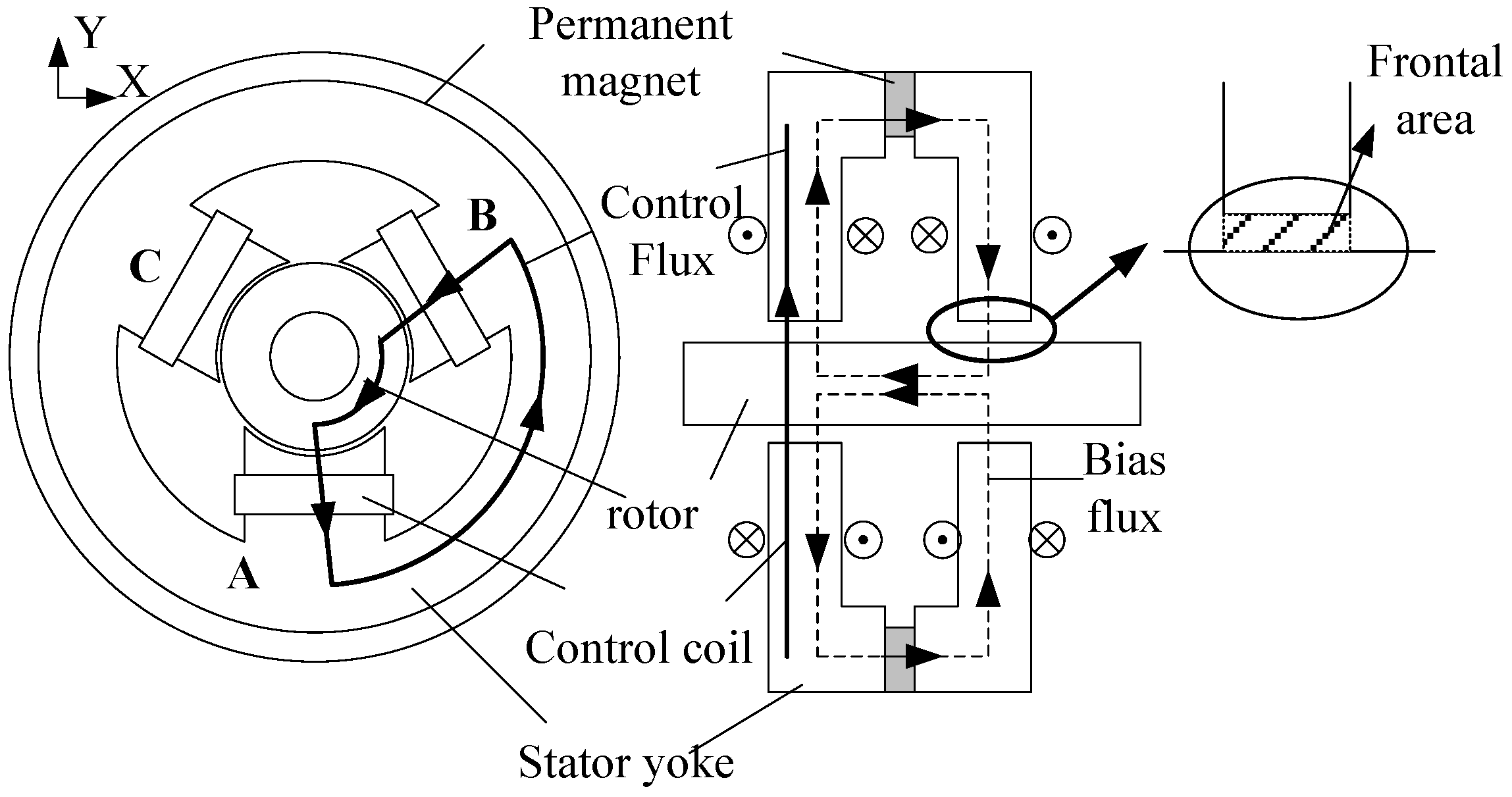
2.1. Configuration and Flux Path of Three-pole Radial HMB

Figure 1 shows the configuration and flux path of the three-pole radial HMB. In Figure 1, it can be seen that the three-pole radial HMB has two symmetrical stators. Each stator has three poles, and the three poles are uniformly spaced at 120° intervals. The two symmetrical coils are connected in series to form a phase, and three phases are in a star connection. A ring-shape permanent magnet connects two stators. An axial magnetized permanent magnet ring provides bias flux flows through stators, air gaps and rotor, as shown by the dashed lines. Bias flux produces magnetic forces to suspend the rotor at the equilibrium position without disturbances and gravity. The control coils supply control flux as the solid line shows. When the input current is positive, the control flux strengthens the bias flux so that the electromagnetic force becomes stronger (biased magnetic forces and control magnetic force are collectively called electromagnetic force in the following context). When the input current is negative, the control flux weakens the bias flux so that the electromagnetic force becomes weaker. Electromagnetic forces from three poles cooperate to stabilize the rotor. There is no coupling between the control flux and bias flux due to the different flux paths. In order to facilitate the description, the three poles are marked as A, B and C.

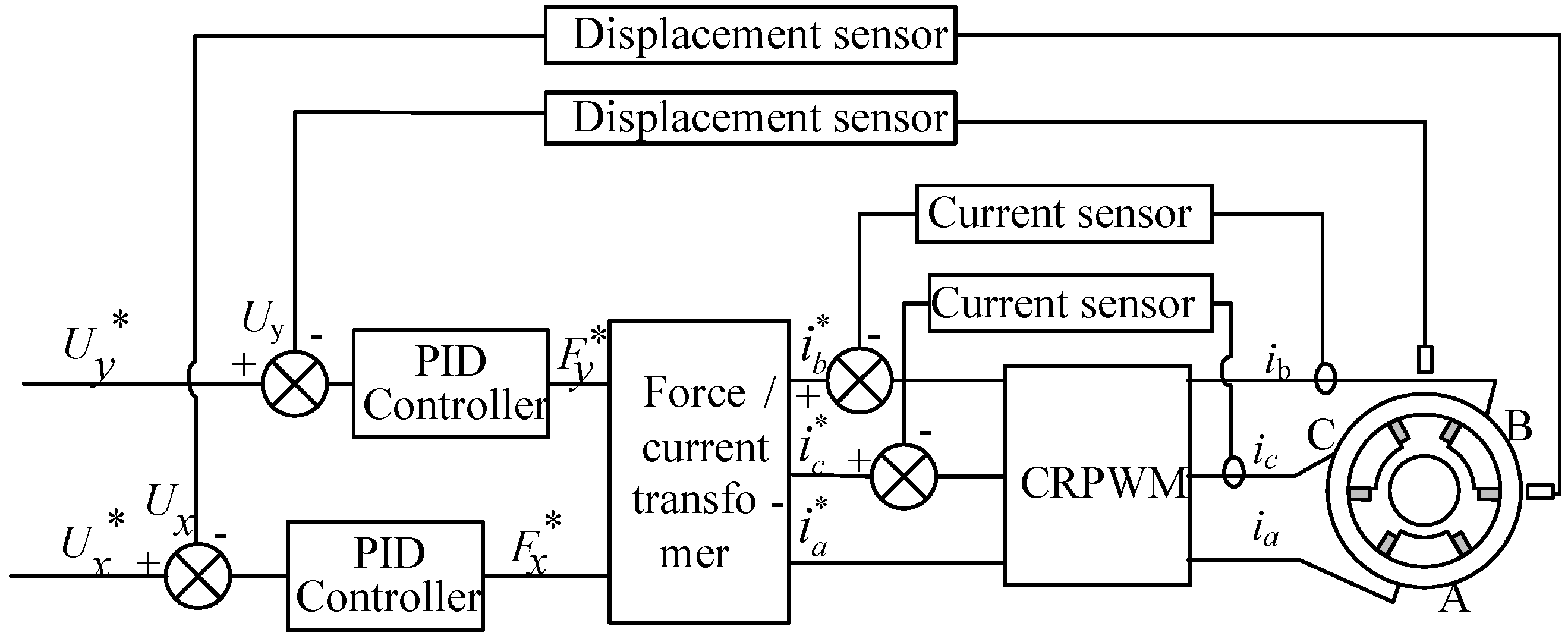
2.2. Control Principle of Three-pole Radial HMB

The control system is a displacement-current double closed-loop feedback control system which comprises controller, three-phase power inverter and displacement sensor modules. Figure 2 shows the control process.

The radial position signals of the rotor are differentially detected by eddy current displacement sensors. Then, the differential signals are compared with the reference values. Through the signal processing circuit, the difference is transferred to PID controller to obtain signals representing the forces. The controller transforms force signals into three phase current signals by force-current transformation and 2/3 coordinate transformation. Then, the three phase currents are taken as reference currents and compared with the input currents of the electromagnets. The input currents are detected by eddy current sensors. Then, the PWM signals are obtained and used to activate the three-phase power inverter. Furthermore, the desired currents can be generated and the desired suspension forces can be produced.

3. Mathematical Model Based on Edge Effect

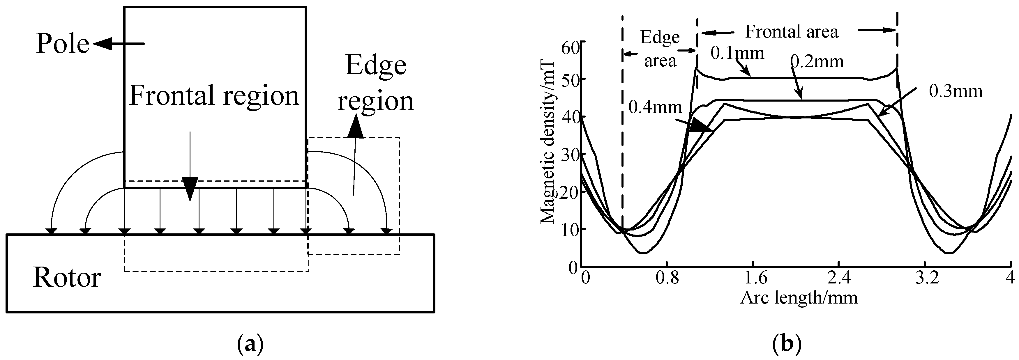
3.1. Edge Effect

The edge effect depicted in Figure 3 indicates that a small part of flux, which is produced by coils and permanent magnets, flows through the edge regions. The flux generates an attractive force between the rotor and stator, which will cause the total electromagnetic force to be stronger than it deduced by the conventional equivalent magnetic circuit method which only considers the flux flows through the frontal region.

Figure 3a shows a schematic diagram of the edge effect. Figure 3b implies that the edge effect becomes stronger as the length of air gap gets larger. If neglected, the edge effect will lead to an increased calculation error. Therefore, it is significant to take the edge effect into consideration in the modelling process of magnetic bearings, especially for large electric drives.

The general method to calculate edge effects is to select empirical value [25]. However, the value selection is difficult and totally depends on the structure of the magnetic bearings, which makes it application-specific, i.e. the method can only applied to a specific type of bearing. Thus, an efficient method is direly needed to evaluate the influence of edge effects.

In Figure 4, pole A is taken as an example to show the flux distribution of the edge effect. The dashed lines, which actually do not exist, are used to distinguish different edge sub-regions. In this three-dimensional figure, it can be seen that edge flux is distributed symmetrically with regard to the pole centre. According to the magnetic field division method [26], the flux around the pole is divided into seven sub-regions (asymmetrical parts are not involved in calculation). As Figure 4 shows, region 1 represents the frontal region of the pole, whose permeance is G₁; regions 2 and 6, whose permeance are G₂ and G6, are shaped like a quarter of a cylinder; regions 3 and 7 are the same as a quarter of a hollow cylinder, whose permeance are G₃ and G₇; region 4 is 1/8 of the sphere, whose permeance is G₄ and region 5 is 1/8 of the hollow sphere, whose permeance is G₅.

3.2. Modeling for Three-pole Radial HMB Based on Edge Effect

The three-pole radial HMB is investigated in this paper. Cartesian coordinates are used and the Y-axis coincides with the reverse direction of pole A. Pole B and pole C are arranged anticlockwise as Figure 1 reveals. A magnetic circuit considering edge effect is established as Figure 5 shows. 2θ and l represent the arc and axial length of the pole, respectively.

where G_A, G_B, G_C are the permeance of the frontal regions of different poles; G_S denotes the total permeance of the edge regions; F_pm is the magnetomotive force and decided by the material properties of the permanent magnet; G₀ is the inner permeance of the permeant magnet. Φ indicates the flux flows through different poles; A, B, C are three poles in the stators. 1 means one of stators and 2 means the other. NI_A, NI_B, NI_C are magnetomotive forces produced by the control coils of different poles. The following assumptions are made for simplicity:

(1)

Arc and axial length of the rotor are much larger than the arc and axial lengths of the poles so the surface of the rotor and the poles are treated as flat; the air gap related to the same pole is uniform.

(2)

The shapes of regions are standard.

(3)

The eddy current effect is neglected.

(4)

The permeability of the stator and the rotor is infinite.

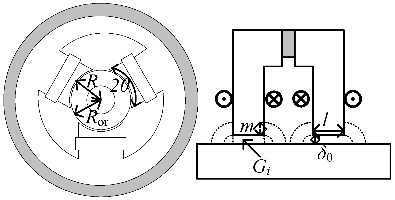
3.2.1. The Length from Pole to Rotor in Eccentric Condition

Due to the existence of air gaps, rotor eccentricity is inevitable. It should be considered in the modeling process. Air gaps are equally without eccentricity. When eccentricity happens, we take x as the eccentric length along the X-axis, and take y as the eccentric length along Y-axis. The eccentric angle α is expressed as follows [16]:

$$\alpha =\arctan (y/x)$$

(1)

The eccentricity ratio ξ can be calculated as follows:

$$\xi =\frac{\sqrt{x^2+y^2}}{{\delta }_0}$$

(2)

Considering the rotor eccentricity, the length of air gap in the angle of ω can be expressed as follows:

$$\delta (\omega )={\delta }_0(1-\xi \cos (\omega -\alpha ))$$

(3)

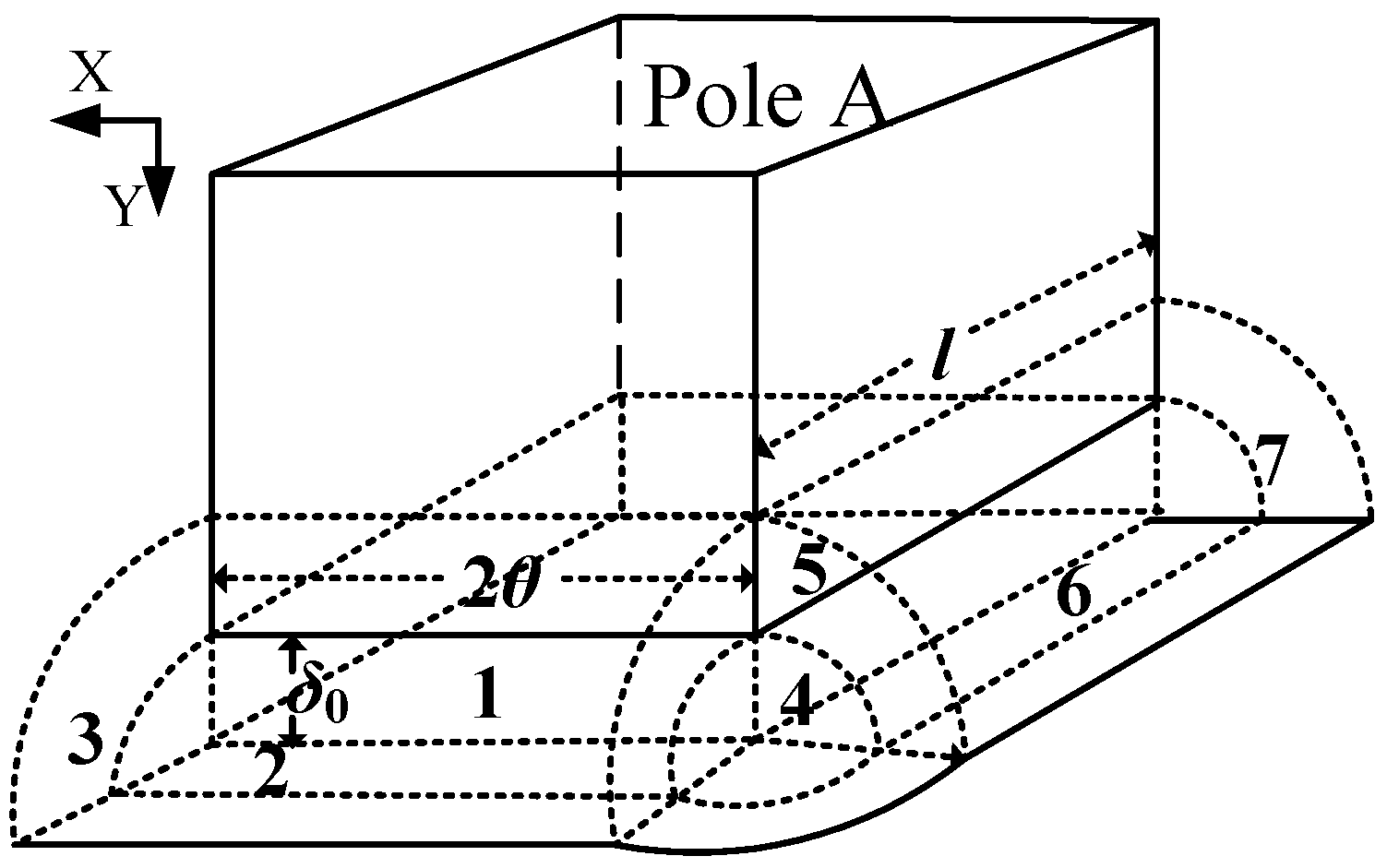
3.2.2. Permeance of Different Regions

The formula to calculate permeance can be written as:

$$G=\frac{{\mu }_{0}S}{{\delta }_{\mathrm{a}\mathrm{v}}}=\frac{{\mu }_{0}V}{{\delta }_{\mathrm{a}\mathrm{v}}^2}$$

(4)

where δ_av is the average physical length of air gaps; S denotes the region of flux distribution; V is the volume of flux distribution; μ₀ is the permeability of vacuum.

Figure 6 shows dimensions of the HMB, which are needed in the calculation of the permeance of air gaps. R is the length between the center of rotor and the frontal face of pole; R_or is the outer radius of the rotor; 2θ is the arc length of the single pole; δ₀ is the length of air gaps without eccentricity; l is the axial length of the pole and m is the radial length considering the edge effect distribution. Here, m = 2δ₀.

Take pole B as an example, the permeance of different edge regions are listed as follows:

The permeance of region 1 can be written as:

$$G_1=\frac{{\mu }_{0}S}{{\delta }_{\text{av}}}=\frac{2R\theta l{\mu }_0}{\delta ({30}^{\circ })}$$

(5)

where 30^° is represents the angle between pole B and X-axis. It changes with relative position.

The minimum air gap length of region 2 is δ(30^°) and the maximum is 1.57δ(30^°). Thus, by the graphing method, the average length is 1.22δ(30^°). The permeance of region 2 is listed as follows:

$$G_2=\frac{{\mu }_{0}V}{{\delta }_{\mathrm{a}\mathrm{v}}^2}=\frac{2R\theta \mathsf{\pi }{\mu }_0}{5.9536}$$

(6)

The permeance of region 3 is:

$$G_3=\frac{{\mu }_{0}S}{{\delta }_{\mathrm{a}\mathrm{v}}}=\frac{2R\theta {\mu }_0}{\mathsf{\pi }}$$

(7)

The permeance of regions 4, 5, 6 and 7 can be obtained in the same way:

$$\{\begin{array}{l}{G}_4=\frac{{\mu }_0\mathsf{\pi }\delta (\omega )}{10.61}\\ G_5={\mu }_0\delta (\omega )\\ G_6=\frac{{\mu }_0\mathsf{\pi }l}{5.95}\\ G_7=\frac{{\mu }_{0}l}{\mathsf{\pi }}\end{array}$$

(8)

Therefore, the total permeance can be deduced as follows:

$$\begin{array}{l}{\displaystyle \sum G=G_1}+2(G_2+G_3)+4(G_4+G_5)+2(G_6+G_7)\\ = \frac{2R\theta {\mu }_{0}l}{\delta (\omega )}+1.7{\mu }_0(2R\theta +l)+5.2{\mu }_0\delta (\omega )\end{array}$$

(9)

In Figure 5, it can be seen that: G_s = 1.7μ₀(2Rθ + l) + 5.2μ₀δ(ω).

After determining the dimensions of the HMB, the corresponding R, l, 2θ are confirmed. Equation (8) shows that, within the constraints of this model, the permeance of the edge regions is only a function of the length of the air gap.

Besides, the inner permeance of the permanent magnet is:

$$G_0=\frac{{\mu }_0{S}_{\mathrm{p}\mathrm{m}}}{l_{\mathrm{p}\mathrm{m}}}$$

(10)

where S_pm is area of the permeant magnet; l_pm is the length of permanent magnet in the magnetized direction. Since poles A, B, and C are positioned symmetrically, the expressions of permeance of three poles can be deduced as follows:

$$\{\begin{array}{c}{\Sigma }_{\mathrm{A}}G=\frac{2R\theta l{\mu }_0}{\delta ({270}^{\circ })}+1.7{\mu }_0(2R\theta +l)+5.2{\mu }_0\delta ({270}^{\circ })\\ {\Sigma }_{\mathrm{B}}G=\frac{2R\theta l{\mu }_0}{\delta ({30}^{\circ })}+1.7{\mu }_0(2R\theta +l)+5.2{\mu }_0\delta ({30}^{\circ })\\ {\Sigma }_{\mathrm{C}}G=\frac{2R\theta l{\mu }_0}{\delta ({150}^{\circ })}+1.7{\mu }_0(2R\theta +l)+5.2{\mu }_0\delta ({150}^{\circ })\end{array}$$

(11)

3.2.3. Magnetomotive Force of Permanent Magnet

The magnetomotive force of a permanent magnet is:

$$F_{\mathrm{p}\mathrm{m}}=H_{\mathrm{p}\mathrm{m}}{l}_{\mathrm{p}\mathrm{m}}$$

(12)

where H_pm is magnetic field intensity of a permanent magnet;

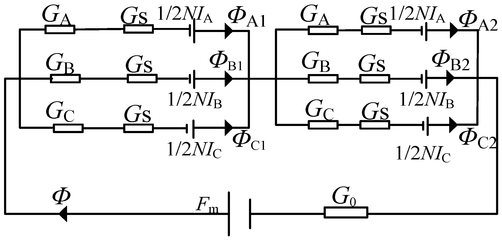
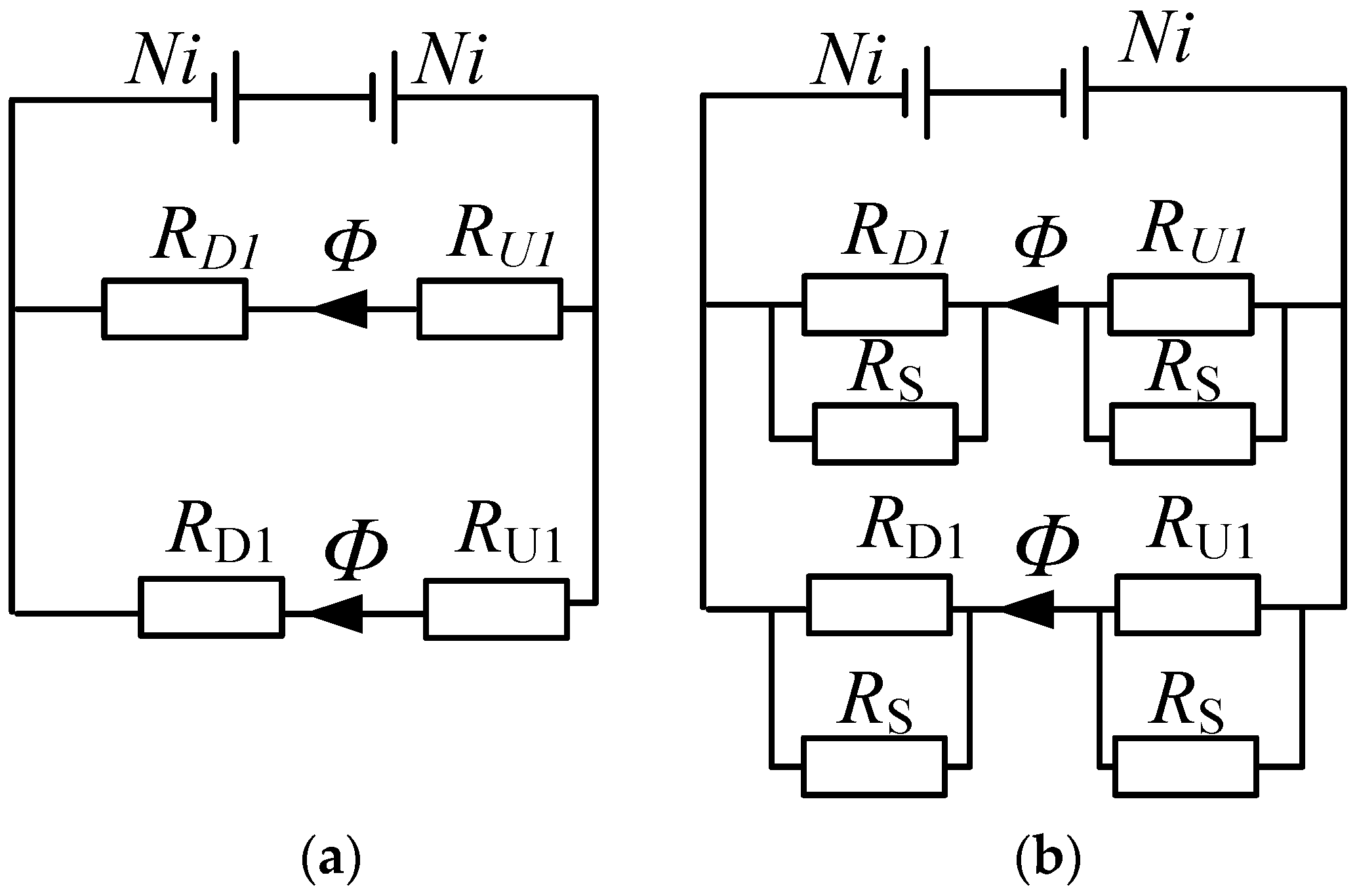
3.2.4. Calculation of Flux and Suspension Force

According to the mathematical relationship between permeance and flux, the flux of the three poles can be acquired as follows:

$$\{\begin{array}{c}{\Phi }_{\mathrm{A}1}={\Phi }_{\mathrm{A}2}=\frac{1}{2\sigma }{F}_{\mathrm{p}\mathrm{m}}({\Sigma }_{\mathrm{A}1}G+G_0)+\frac{1}{2\sigma }N{i}_{\mathrm{A}}{\Sigma }_{\mathrm{A}2}G\\ {\Phi }_{\mathrm{B}1}={\Phi }_{\mathrm{B}2}=\frac{1}{2\sigma }{F}_{\mathrm{p}\mathrm{m}}({\Sigma }_{B1}G+G_0)+\frac{1}{2\sigma }N{i}_{\mathrm{B}}{\Sigma }_{B2}G\\ {\Phi }_{\mathrm{C}1}={\Phi }_{\mathrm{C}2}=\frac{1}{2\sigma }{F}_{\mathrm{p}\mathrm{m}}({\Sigma }_{\mathrm{C}1}G+G_0)+\frac{1}{2\sigma }N{i}_{\mathrm{C}}{\Sigma }_{\mathrm{C}2}G\end{array}$$

(13)

where σ is leakage coefficient; N is number of coil turns; i is the control current of coils; Σ_A1G=Σ_A2G, Σ_B1G=Σ_B2G, Σ_C1G=Σ_C2G.

The angles between poles and X-axis in eccentric condition can be expressed as follows:

$$\{\begin{array}{l}{\rho }_{\mathrm{A}}=\arctan (\frac{-({\delta }_0+R_{or})-y}{-x})\\ {\rho }_{\mathrm{B}}=\arctan (-\frac{({\delta }_0+R_{\mathrm{o}\mathrm{r}})\sin ({30}^{\circ })-y}{({\delta }_0+R_{\mathrm{o}\mathrm{r}})\cos ({30}^{\circ })-x})\\ {\rho }_{\mathrm{C}}=\arctan (\frac{({\delta }_0+R_{\mathrm{o}\mathrm{r}})\sin ({150}^{\circ })-y}{({\delta }_0+R_{\mathrm{o}\mathrm{r}})\cos ({150}^{\circ })-x})\end{array}$$

(14)

where ρ_A is the angle between pole A and X-axis; ρ_B is the angle between pole B and X-axis; ρ_C is the angle between pole C and X-axis.

The electromagnetic force expression is:

$$F_j=\frac{{\Phi }_j{}^2}{2{\mu }_{0}S}$$

(15)

where j = A, B, C.

Based on the formula above, in the same direction, resultant force can be deduced according to the relationship between flux and electromagnetic forces:

$$F_j=\frac{{\Phi }_{j1}^2}{2{\mu }_{0}S}+\frac{{\Phi }_{j2}^2}{2{\mu }_{0}S}=\frac{{\Phi }_{j1}^2}{{\mu }_{0}S}=\frac{{\Phi }_{j2}^2}{{\mu }_{0}S}$$

(16)

Thus the suspension forces in the X-axis and Y-axis direction are expressed as follows under eccentric conditions:

$$\{\begin{array}{l}{F}_{\mathrm{x}}=F_{\mathrm{B}}\cos ({\rho }_{\mathrm{B}})-F_{\mathrm{A}}\sin ({\rho }_{\mathrm{A}})-F_{\mathrm{C}}\cos ({\rho }_{\mathrm{C}})\\ F_{\mathrm{Y}}=F_{\mathrm{B}}\sin ({\rho }_{\mathrm{B}})-F_{\mathrm{A}}\cos ({\rho }_{\mathrm{A}})+F_{\mathrm{C}}\sin ({\rho }_{\mathrm{C}})\end{array}$$

(17)

Specially, when i_A = −2i_B = −2i_C, the suspension forces can be expressed as equation (18):

$$\{\begin{array}{l}{F}_{\mathrm{X}}=0\\ F_{\mathrm{Y}}=\frac{1}{2}{F}_{\mathrm{B}}+\frac{1}{2}{F}_{\mathrm{C}}-F_{\mathrm{A}}\end{array}$$

(18)

3.3. Analysis of Generality

3.3.1. Magnetic Bearings with Different Dimensions

Equation (9) has indicated that the distinction between the proposed model and the conventional equivalent magnetic circuit model is that there is an additional term of 1.7μ₀(2Rθ + l) + 5.2μ₀δ(ω) in the former. This term stands for the permeance of edge regions. It is only related to the specific parameters of magnetic bearings. That is to say, the term is the function of the length of the air gap when the parameters of magnetic bearing are determined. A solution to calculate the length of air gap has been presented above. The additional term is equal everywhere while the rotor in the equilibrium position, but it changes in the presence of eccentricity.

3.3.2. Magnetic Bearings with Different Configurations

The equivalent magnetic circuit method is established based on the flux path. On the basis of the equivalent magnetic circuit method, the model established in this paper begins by analyzing the flux distribution of a single pole. Due to the consistency among poles, the result of the analysis is easily applied to a range of practical design applications. From the derivation process, it can be seen that the only work needed to be done is the addition of 1.7μ₀(2Rθ + l) + 5.2μ₀δ(ω) to the frontal permeance no matter the number of poles the HMB have. Taking the four-pole type of HMB in [27] as an example, the common control magnetic circuit is shown in Figure 7a and the equivalent magnetic circuit considering the edge effect is shown in Figure 7b.

In Figure 7, R_S is the total reluctance of the edge regions of a single pole, and satisfies the mathematical relation: 1/R_S = G_S.

3.3.3. Used in Other Fields of Magnetic Bearings

The edge effect researched in this paper has no conflict with other effects like eddy current effect, flux saturation effect and so on. Taking the eddy current effect as an example, after demonstrating the effect of the eddy current, [10] proposed a new magnetic bearing design involving calculation of permeance. According to the illustration above, if the edge effect is considered, the only work that needs to be done is add a modified additional term to the frontal permeance of the poles to act as total permeance in the calculation process.

From the explanations above, the established model modifies the conventional model and appends an additional term which considers the edge effect. It simplifies the counting procedure so that redundant calculation is avoided. The new model combines principles of geometry and electromagnetism, and is independent of the configuration of HMBs, which makes it applicable to different HMBs.

4. Experiment and Analysis

In order to verify the validity of the proposed model, simulation and experiment are performed on a three-pole radial HMB with a maximum capacity of 50 N. The finite element analysis (FEA) simulation is conducted in static magnetic field. The specifications of the three-pole HMB are listed in

Table 1. Specifications of the three-pole radial HMB.

Parameters	Values
Outer diameter of rotor	19 mm
Inner diameter of rotor	9 mm
Outer diameter of stator yoke	64 mm
Inner diameter of stator yoke	40 mm
Inner diameter of permanent magnet	53.4 mm
Inner diameter of Permanent magnet	64 mm
Axial length of pole	10 mm
Axial length of rotor	25 mm
Thickness of permanent magnet	2.5 mm
Arc length of pole	π/2 rad
Length of air gap	0.5 mm
Turns of coil	100 At
Cross-sectional area of permanent magnet	265 mm2
Saturation magnetic flux	0.9 T
Outer diameter of rotor	19 mm

.

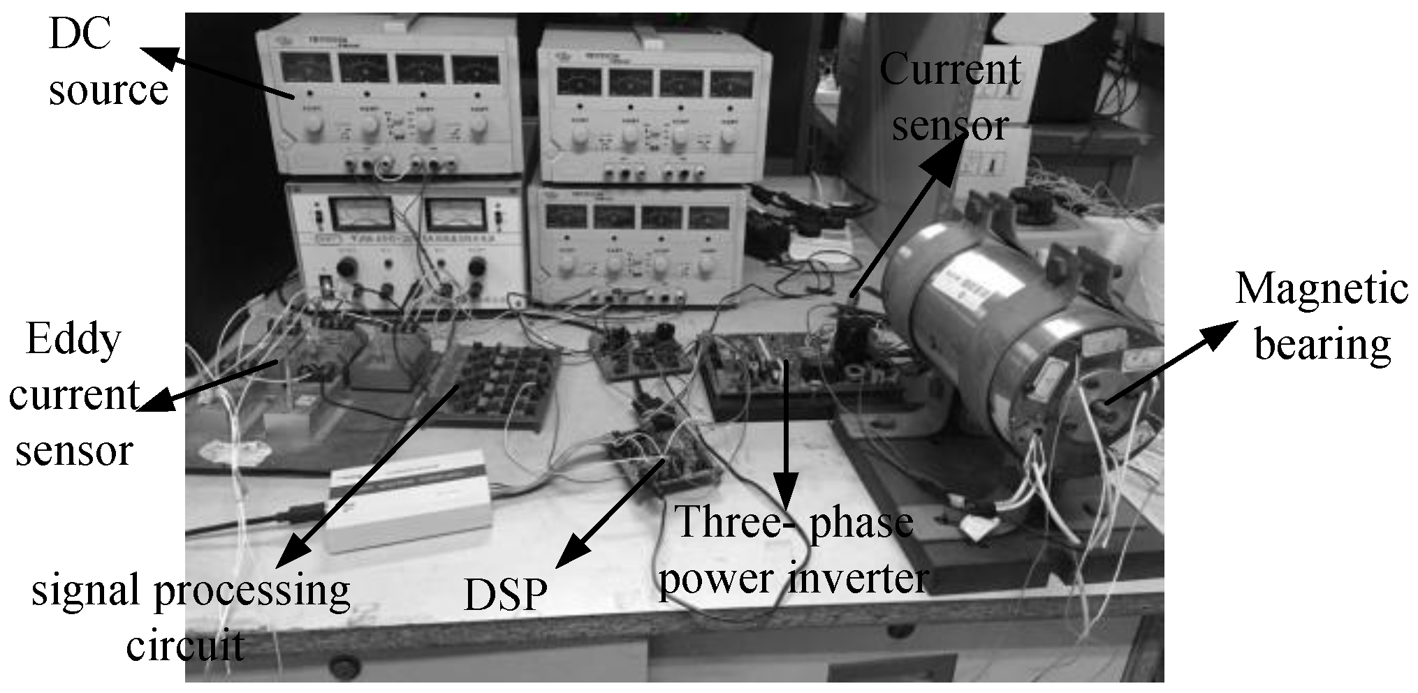
4.1. Introduction of the Three-pole Radial HMB Experimental Rig

The experimental system comprises a controller module, a sensor module, a three-phase power inverter module and the three-pole radial HMB. The controller is operating on a TMS320F2812 digital signal processor (TI Inc.: Dallas, TX, USA). Sensor module include an eddy current displacement sensors and current sensors. The control process has been depicted in Section 2 in detail. Figure 8 shows the experimental rig.

The length of air gap is designed to be 0.5 mm. However, to protect the experimental instruments and people around in some extreme case, an auxiliary bearing was adopted to limit the rotor vibration to a 0.25 mm circle. The auxiliary bearing is placed on both ends of the bearing so that it has no effect on the three-pole radial HMB. The eddy current displacement sensors used in this experimental rig are installed in the directions of the axes to detect the differential displacement signals. The differential signals can avoid any errors caused by special conditions like temperature drift, circular motion around a single sensor and so on. The output voltage of the displacement sensors changes from −2 V to −18 V, which exceeds the input range of the analogy-to-digital converter. Thus, the differential signals need to be converted by a signal processing circuit. To simplify the experimental procedure, when the rotor is located at a −0.25 mm, the output voltage of the displacement sensor is set to 0.4 V. When it is located at 0.25 mm, the output voltage is set to 2.6 V, so the sensors will output 1.5 V when the rotor at the equilibrium position. Due to the particularity of the three-pole radial HMB, a three-phase power inverter is employed to activate the electromagnets. Due to the fact the three electromagnets are connected in a star arrangement, according to the Kirhhoff’s Current Law, the input currents equal the output currents. The currents in the electromagnets are detected by current sensors to constitute a closed-loop control system.

Due to the nonlinearity of the three-pole radial HMB, the rotor is limited to operating around the equilibrium position so that the calculation values can match the experiment values. In the three-pole radial HMB, the air gap flux density provided by the permanent magnet ring is 0.45 T. The stator and rotor are made of silicon steel sheets. The flux knee of the BH curve of silicon steel sheet is about 1.5 T. In the design process of the three-pole radial HMB, the maximum flux density of air gap is chosen as 0.9 T, which is far lower than 1.5 T. Therefore, the designed magnetic bearing can work in a relatively linear way, and flux saturation cannot be the reason for any discrepancy between the experimental data and calculated data.

4.2. Analysis of Results

The control variate method is employed in this experiment so that the effect of current and displacement can be analyzed, respectively.

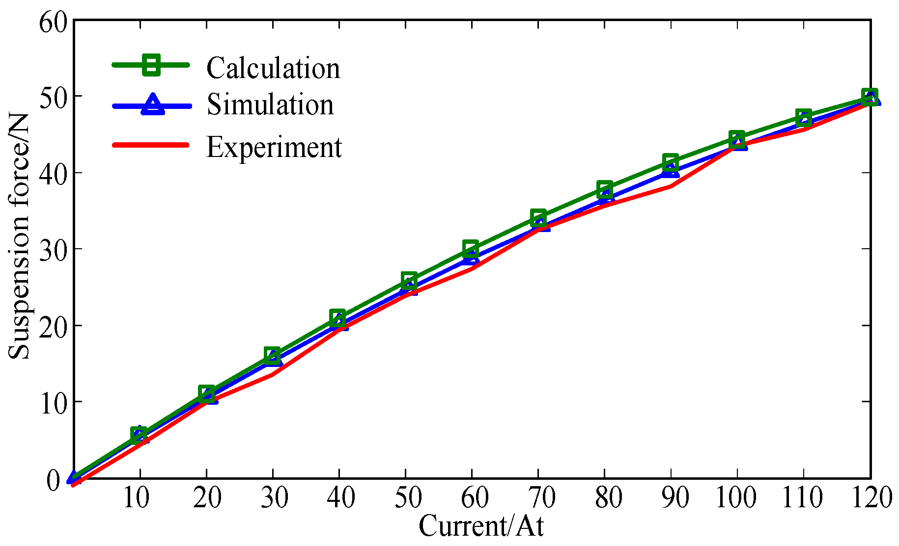
4.2.1. Test of Relationship between Force and Current

This part of experiment aimed to study the relationship between suspension forces and currents. The experimental values are measured by a spring dynamometer. In order to eliminate the effect of eccentricity, the rotor is limited in the equilibrium position. In this condition, by expanding Equation (15) in a Taylor series and ignoring higher order terms, the suspension forces are linearized. Under this assumption, the suspension forces are supposed to be proportional to the current and are expected to be nearly linear. The data relating to the suspension force have been collected and recorded by inputting different currents. To facilitate the measurement, input currents follow the rule that i_A = −2i_B = −2i_C. In this case, due to the fact the suspension force has no component in the X direction, the suspension force in the Y direction represents the total suspension force, and can be directly read by the spring dynamometer. Figure 9 shows the results of our calculation, simulation and experiment. It can be seen that stiffness coefficients of force/current in the proposed model match the experimental results well, and the assumption of linearity is valid over the range studied.

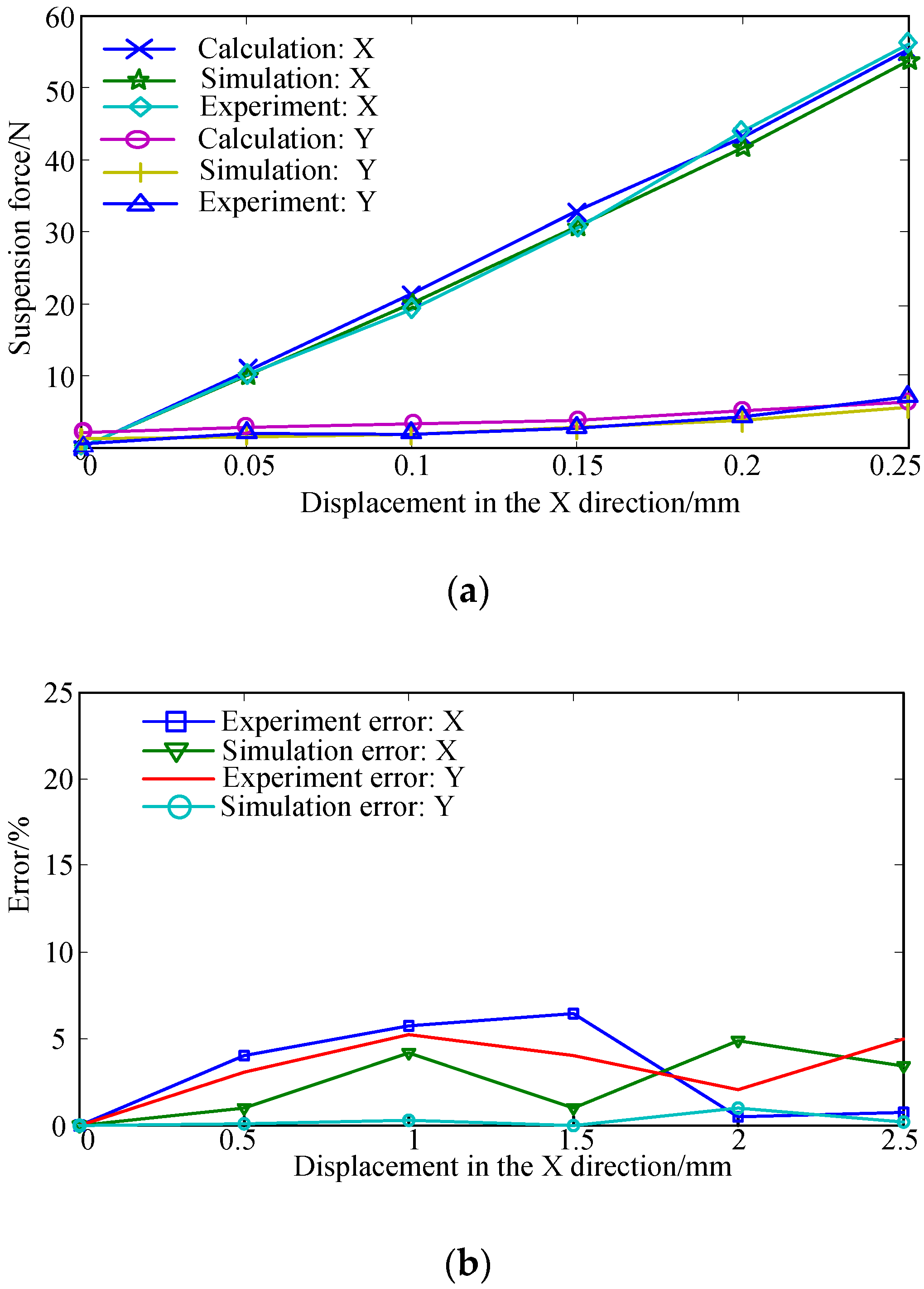
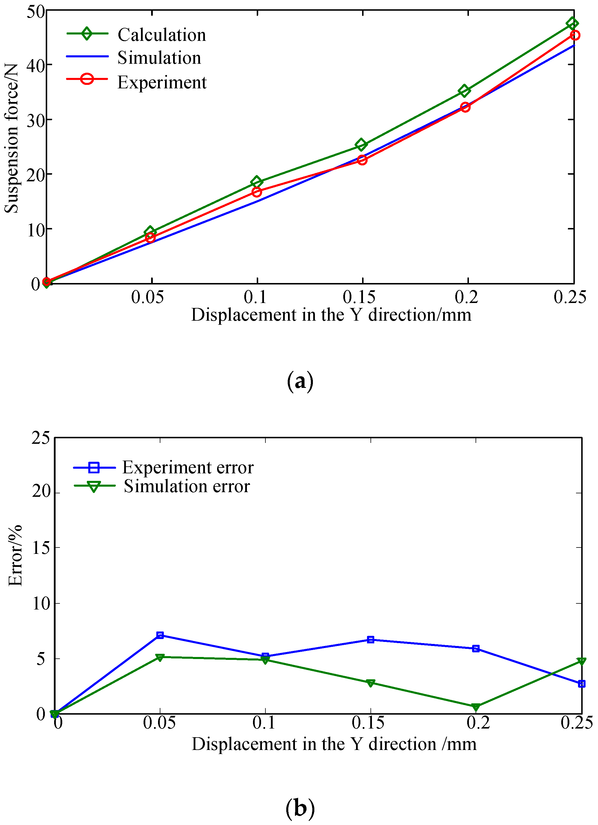
4.2.2. Test of Relationship between Force and Displacement

To study the relationship between the forces and the displacements, the input currents are taken as zero so that the suspension forces are approximatively proportional to the displacements. In this part of the experiment, the spring dynamometer is employed to make the rotor deviate from the equilibrium position. Therefore, the reading of spring dynamometer equals the suspension force under different eccentricity conditions. The displacement is confined in the range of −0.25 mm–0.25 mm in this investigation. However, the tendency of the stiffness coefficient is central symmetry regarding the equilibrium position, so the curve in the negative direction is omitted. Figure 10a and Figure 11a show the suspension forces under different eccentricity conditions. Due to the fact the calculation curve is very close to the simulation curve and experimental curve, error figures are also provided. Figure 10b and Figure 11b illustrate the experimental error and simulation error under different eccentric conditions. The calculation error can be obtained in three steps: firstly, one works out the difference between calculated and experimental values. Secondly, one works out the ratio of the difference with the experimental values. Finally, the calculation error is obtained by transforming the ratio into a percentage form. The experimental error can be obtained in the same way. From the figures, the stiffness coefficients of force/displacement obtained by simulations and experiments are consistent with the result obtained by the proposed model.

Notice that when eccentricity occurs in the Y direction, the suspension fore in the X direction is not shown in Figure 10a, because its value is zero. The reason is that electromagnetic forces of pole B and pole C in the X-axis direction are offset, and the force from pole A has no component in the X-axis direction. In addition, when eccentricity occurs in the X direction, Figure 11a,b tell us that the suspension force in the Y-axis direction changes slightly. The reason is that the eccentricity is far less than the arc length of the rotor so the value obtained by Equation (14) basically remains unchanged, and the value of the suspension force in the Y-axis direction obtained by Equation (17) changes slightly. Figure 11a proves the correctness of Equation (14) and Equation (17).

4.2.3. Error Analysis

Figure 9, Figure 10a,b and Figure 11a,b reflect a phenomenon whereby the force values calculated by the proposed model are larger than the FEA simulation values and the experimental values. The reason is that proposed model neglects the eddy current. The magnetic field produced by the eddy current reduces the original magnetic field and leads to the actual flux becoming smaller. Those elements will weaken the total force and cause differences between the theoretical calculation values, FEA simulation values and experimental values. However, from Figure 10b and Figure 11b, it can be seen that the largest difference between the calculated and FEA simulation values is less than 5%, and largest difference between the calculated and experimental values is less than 7%.

5. Conclusions

In this paper, a mathematical model of a three-pole radial HMB considering the edge effect is proposed. After analyzing the distribution features of edge flux around a single pole, the edge effect calculation is carried out by the magnetic field division method and superposition principle. Furthermore, the generality of the proposed model is presented. It implies that the calculation of edge effects is only related to the configuration and parameters of a single pole, and is isolated with the other configurations and parameters of the three-pole radial HMB. Besides, its calculation has no conflict with other effects so that it can be used in studying other effects to obtain more accurate suspension forces. The precision of the established model was verified by finite element analysis and experiments. The error between the theoretical calculation value and the FEA simulation value is less than 5%, and the error between the theoretical calculation value and the experimental value is less than 7%.

References

1. Hou, E.Y.; Liu, K. A Novel Structure for Low-Loss Radial Hybrid Magnetic Bearing. IEEE Trans. Magn. 2011, 47, 4725–4733. [Google Scholar]
2. Fang, J.C.; Sun, J.J.; Xu, Y.L.; Wang, X. A New Structure for Permanent-Magnet-Biased Axial Hybrid Magnetic Bearings. IEEE Trans. Magn. 2009, 45, 5319–5325. [Google Scholar]
3. Schuhmann, T.; Hofmann, W.; Werner, R. Improving Operational Performance of Active Magnetic Bearings Using Kalman Filter. IEEE Trans. Magn. 2015, 59, 821–829. [Google Scholar]
4. Bachovchin, K.D.; Hoburg, J.F.; Post, R.F. Magnetic Fields and Forces in Permanent Magnet Levitated Bearings. IEEE Trans. Magn. 2012, 48, 2112–2120. [Google Scholar] [CrossRef]
5. Ji, L.; Xu, L.X.; Jin, C.W. Research on a Low Power Consumption Six-Pole Heteropolar Hybrid Magnetic Bearing. IEEE Trans. Magn. 2013, 49, 4918–4926. [Google Scholar] [CrossRef]
6. Pichot, M.A.; Kajs, J.P.; Murphy, B.R.; Ouroua, A.; Rech, B.M.; Hayes, R.J.; Beno, J.H.; Buckner, G.D.; Palazzolo, A.B. Active magnetic bearings for energy storage systems for combat vehicles. IEEE Trans. Magn. 2001, 37, 318–323. [Google Scholar] [CrossRef]
7. Han, B.C.; Zhen, S.Q.; Wang, X.; Yuan, Q. Integral Design and Analysis of Passive Magnetic Bearing and Active Radial Magnetic Bearing for Agile Satellite Application. IEEE Trans. Magn. 2012, 48, 1959–1966. [Google Scholar]
8. Kim, S.H.; Shin, J.W.; Ishiyama, K. Magnetic Bearings and Synchronous Magnetic Axial Coupling for the Enhancement of the Driving Performance of Magnetic Wireless Pumps. IEEE Trans. Magn. 2014, 50, 4003404. [Google Scholar] [CrossRef]
9. Kimman, M.H.; Langen, H.H.; Schmidt, R.H. A miniature milling spindle with active magnetic bearings. Mechatronics 2010, 20, 224–235. [Google Scholar] [CrossRef]
10. Usman, I.; Paone, M.; Smeds, K.; Lu, X.D. Radially biased axial magnetic bearings/motors for precision rotary-axial spindles. IEEE/ASME Trans. Mechatronics 2011, 16, 411–420. [Google Scholar] [CrossRef]
11. Zhang, W.Y.; Zhu, H.Q. Key Technologies and Development Status of Flywheel Energy Storage System. Trans. China Electrotech. Soc. 2011, 26, 141–146. [Google Scholar]
12. Schweitzer, G.; Maslen, E.; Okada, Y. Magnetic Bearings: Theory, Design, and Application to Rotating Machinery; Springer Press: Berlin, Germany, 2009. [Google Scholar]
13. Hsu, C.T.; Chen, S.L. Exact Linearization of a Voltage-Controlled 3-Pole Active Magnetic Bearing System. IEEE Trans. Control Syst. Technol. 2002, 10, 618–625. [Google Scholar]
14. Chen, S.L.; Chen, S.H.; Yan, S.T. Experimental Validation of a Current-Controlled Three-Pole Magnetic Rotor-Bearing System. IEEE Trans. Magn. 2005, 41, 99–112. [Google Scholar] [CrossRef]
15. Xie, Z.Y.; Zhu, H.Q.; Sun, Y.K. Structure and control of AC-DC three-degree-of-freedom hybrid magnetic bearing. In Proceedings of the 8th International Conference on Electrical Machines and Systems, Nanjing, China, 27–29 September 2005; pp. 1801–1806.
16. Yang, H.; Zhao, R.X.; Tang, Q.B. Study on inverter-fed three-pole active magnetic bearing. In Proceedings of Twenty-First Annual IEEE Applied Power Electronics Conference and Exposition, Dallas, TX, USA, 19–23 March 2006; pp. 1576–1581.
17. Zhang, W.Y.; Zhu, H.Q. A novel modeling method for radial suspension forces of AC magnetic bearings. Chin Sci Bull (Chin Ver) 2012, 57, 976–986. [Google Scholar]
18. Zhang, Y.P.; Liu, S.Q.; Li, H.W.; Fan, Y.P. Calculation of Radial Electromagnetic Force of Axial Hybrid Magnetic Bearing Based on Magnetic Circuit Analysis. Trans. China Electrotech. Soc. 2012, 27, 137–142. [Google Scholar]
19. Han, B.C.; Zheng, S.Q.; Le, Y.; Xu, S. Modeling and Analysis of Coupling Performance between Passive Magnetic Bearing and Hybrid Magnetic Radial Bearing for Magnetically Suspended Flywheel. IEEE Trans. Magn. 2013, 49, 5356–5370. [Google Scholar] [CrossRef]
20. Zhang, W.Y.; Zhu, H.Q. Influence of eddy effect to the parameter design and optimized design for magnetic bearing. Electr. Mach. Control 2012, 16, 67–77. [Google Scholar]
21. Kang, K.; Palazzolo, A. Homopolar Magnetic Bearing Saturation Effect on Rotating Machinery Vibration. IEEE Trans. Magn. 2012, 48, 1984–1994. [Google Scholar] [CrossRef]
22. Wang, X.G.; Bin, M. Study on the Centripetal Effect of a Magnetic Bearing. In Proceeding of International Conference Electrical and Control Engineering, Wuhan, China, 25–27 June 2010; pp. 2135–2138.
23. Zhang, Y.P.; Xue, B.W.; Liu, S.Q.; Li, H.W. Calculation of electromagnetic force of axial hybrid magnetic bearing based on fringe effect of magnetic flux. Electr. Mach. Control 2014, 18, 54–67. [Google Scholar]
24. Huang, L.; Zhao, G.Z.; Nian, H.; He, Y.K. Modeling and design of permanent magnet biased radial-axial magnetic bearing by extended circuit theory. In Proceeding of International Conference on Electrical Machines and Systems, Seoul, Korea, 8–11 October 2007; pp. 1502–1507.
25. Lu, J.Y.; Ma, W.M.; Li, L.R. Research on Longitudinal End Effect of High Speed Long Primary Double-sided Linear Induction Motor. Chin. Soc. Elec. Eng. 2008, 28, 73–78. [Google Scholar]
26. Xia, T.W.; Ding, M.D. Electronmechanics, China; China Machine Press: Beijing, China, 2011; pp. 79–87. [Google Scholar]
27. Liu, X.X.; Dong, J.Y.; Du, Y.; Shi, K.; Mo, L.H. Design and Static Performance Analysis of a Novel Axial Hybrid Magnetic Bearing. IEEE Trans. Magn. 2014, 50, 8300404. [Google Scholar] [CrossRef]
Figure 1. Configuration and flux path of the three-pole radial HMB.
Energies 09 00345 g001
Figure 2. Control block diagram of three-pole radial HMB.
Energies 09 00345 g002
Figure 3. (a) Schematic diagram of the edge effect. (b) Relationship between the edge effect flux density distribution and the length of the air gap.
Energies 09 00345 g003
Figure 4. Region division of the edge flux.
Energies 09 00345 g004
Figure 5. Magnetic circuit considering edge effect.
Energies 09 00345 g005
Figure 6. Dimensions of each part of the three-pole radial HMB.
Energies 09 00345 g006
Figure 7. (a) Common equivalent magnetic circuit. (b) Equivalent magnetic circuit considering the edge effect.
Energies 09 00345 g007
Figure 8. Experimental system of the three-pole radial HMB.
Energies 09 00345 g008
Figure 9. Comparison among calculation, simulation and experiment results.
Energies 09 00345 g009
Figure 10. (a) Suspension force related to eccentricity along the Y-axis (b) Error comparison between experiment and simulation
Energies 09 00345 g010
Figure 11. (a) Suspension force related to eccentricity along the X-axis (b) Error comparison between experiment and simulation
Energies 09 00345 g011