A High-Performance Adaptive Incremental Conductance MPPT Algorithm for Photovoltaic Systems

Abstract

The output characteristics of photovoltaic (PV) arrays vary with the change of environment, and maximum power point (MPP) tracking (MPPT) techniques are thus employed to extract the peak power from PV arrays. Based on the analysis of existing MPPT methods, a novel incremental conductance (INC) MPPT algorithm is proposed with an adaptive variable step size. The proposed algorithm automatically regulates the step size to track the MPP through a step size adjustment coefficient, and a user predefined constant is unnecessary for the convergence of the MPPT method, thus simplifying the design of the PV system. A tuning method of initial step sizes is also presented, which is derived from the approximate linear relationship between the open-circuit voltage and MPP voltage. Compared with the conventional INC method, the proposed method can achieve faster dynamic response and better steady state performance simultaneously under the conditions of extreme irradiance changes. A Matlab/Simulink model and a 5 kW PV system prototype controlled by a digital signal controller (TMS320F28035) were established. Simulations and experimental results further validate the effectiveness of the proposed method.

1. Introduction

With the increasing problem of environmental pollution and approaching depletion of conventional fossil-fuel energy sources, solar energy, as a clean, environmentally-friendly and abundant energy source is attracting more attention. An effective way of using solar energy is photovoltaic (PV) generation; however, the output characteristics of PV arrays vary with the environment (cell temperature and irradiation). The maximum power point (MPP) tracking (MPPT) techniques are thus employed to harvest the maximum power from PV arrays [1,2]. In recent years, many MPPT strategies have been proposed with differences in complexity, cost, convergence speed, and overall output efficiency [3].

Fractional open-circuit voltage (FOV) [4] and fractional short-circuit current (FSC) [5] methods take advantage of the approximate linear relationship between operating voltage or current at the MPP and open-circuit voltage or short-circuit current of PV arrays; therefore, they are simple and effective ways to track the MPP. FOV [4] and FSC [5] have already been used for PV systems of street lighting, as the precise tracking is unnecessary for it. Nevertheless, these methods have larger power losses, because the open-circuit voltage and the short-circuit current are measured by shutting down or short-circuiting PV arrays periodically. Furthermore, the operating point of FOV [4] and FSC [5] is not the real MPP, technically.

Hill climbing (HC), and perturb and observe (P&O) [6,7,8] methods have been widely studied. The perturbation selections are different for HC and P&O: one is the duty ratio of the power converter [6] and the other one is the voltage of the PV array [7,8]. In fact, they are different realizations of the same concept. HC and P&O [6,7,8] have many merits, such as simple structure, ease of installation and maintenance. However, contradiction appears in choosing the perturbation parameter (duty cycle or reference voltage) in both methods. A larger parameter contributes to a better dynamic performance but excessive power loss at steady state, resulting in a comparatively low efficiency, and vice versa.

In addition, fuzzy logic control [9], sliding-mode control [10], and neural-network methods [11] have also been used for MPPT over the last decades. The fuzzy logic control algorithm [9] is good at handling nonlinear problems without an accurate mathematical model, and good steady state performance can be achieved in varying atmospheric conditions. However, its effectiveness relies a lot on the experience or knowledge of the designer in determining the division of fuzzy field and formulating a fuzzy rule base table. Sliding-mode control [10] improves the dynamic performance greatly, as well as the robustness of the PV system, but its high complexity and implementation cost makes it be seldom applied for the practical system. The neural-network algorithm [11] increases the efficiency of the system by adopting a multilayer structure; however, each kind of PV array has to be specially trained to create the control rules; thus, its limitation is versatility.

The incremental-conductance (INC) [12,13,14,15,16,17,18] method is also often applied in PV systems. It tracks the MPP by comparing the instantaneous and incremental conductance of the PV array. The issue of INC method is similar to P&O. The fixed step size is usually adopted, which determines the accuracy and response speed of MPPT. Thus, a tradeoff has to be made between the tracking speed and steady state performance. Such design dilemma can be settled with variable step size MPPT strategies. The derivative of power to voltage (dP/dV) is used to adjust the step size of MPPT. The step size is increased when the operating point is far from the MPP, and it is decreased gradually when the operating point gets close to the MPP [13]. The fast tracking speed and stable output can be simultaneously achieved by the adjustment of the step size. However, a scaling factor is necessary to ensure the convergence of the MPPT algorithm, and the scaling factor decreases the response speed greatly under rapid change of atmospheric conditions. An incremental-resistance (INR) MPPT algorithm is examined with the modified variable step size [14]. A threshold function is applied to shift between the mode of the fixed step size and the variable step size, and the variable step process is realized by a varying scaling factor. This method acquires fast response and accurate steady state performance, but the heavy computational load and strong non-linearity of the scaling factor restrict its application. In [15], there are two step size adjustment coefficients to reduce the effects to perturbation (duty ratio) under the extreme change of irradiation with less computation, while it does not consider the influence of the initial step size on the performance of the algorithm.

In this paper, a novel INC MPPT method is proposed with the adaptive variation of step size. An adjustment coefficient is adopted to regulate the step size. Therefore, the PV system can keep a large step size when the operating point is far from the MPP and a decreasing step size when the operating point is close to the MPP, even under extreme irradiance change. The proposed method can effectively solve the problem of traditional method not taking into account the stability and dynamic response speed simultaneously when the irradiance changes tremendously. Compared with other variable step size methods, the proposed method also has less complex adjustment coefficient and computation to improve the computing speed. In addition, a method of tuning initial step size is also presented to further improve the dynamic performance. Simulation and experimental results verify the effectiveness of the proposed algorithm.

2. Analysis of the Photovoltaic (PV) System

As shown in Figure 1, a standalone PV system usually consists of three main blocks: PV array, the MPPT control unit and DC-DC converter. Analysis will be conducted for them in the subsequent sections.

2.1. PV Model

A PV array is a nonlinear device, which is modeled as a current source shunted with a diode. Figure 2 illustrates the equivalent circuit of PV array.

The output I-V characteristic is given as:

$$I=I_{ph}-I_s\left\{\exp [\frac{q}{AkT}(V+I{R}_s)]-1\right\}-\frac{V+I{R}_s}{R_{sh}},$$

(1)

$$I_s=I_{sref}{\left(\frac{T}{T_{ref}}\right)}^3\exp [\frac{q{E}_g}{Ak}(\frac{1}{T_{ref}}-\frac{1}{T})],$$

(2)

$$I_{ph}=\left[I_{sref}+K_I(T-25)\right]\lambda /100,$$

(3)

where I is the output current of the PV module in A, and V is the output voltage in V. I_ph is the light-generated current in A, I_s is the diode reverse saturation current in A, q is the electron charge, q = 1.602 × 10⁻¹⁹ C, k is the Boltzmann’s constant, k = 1.381 × 10⁻²³ J/K, A stands for the ideality factor of P-N junction, $1\le A\le 2$, T is the cell temperature in °C, R_s is the intrinsic series resistance in Ω, R_sh is the shunt resistance in Ω, I_sref is the cell reverse saturation current at T_ref, E_g is band gap of silicon, E_g = 1.12 eV (at 25 °C), I_scref is the short circuit current at 25 °C and 1000 W/m², K_I is short circuit current temperature coefficient in A/C, and λ is solar irradiation in W/m².

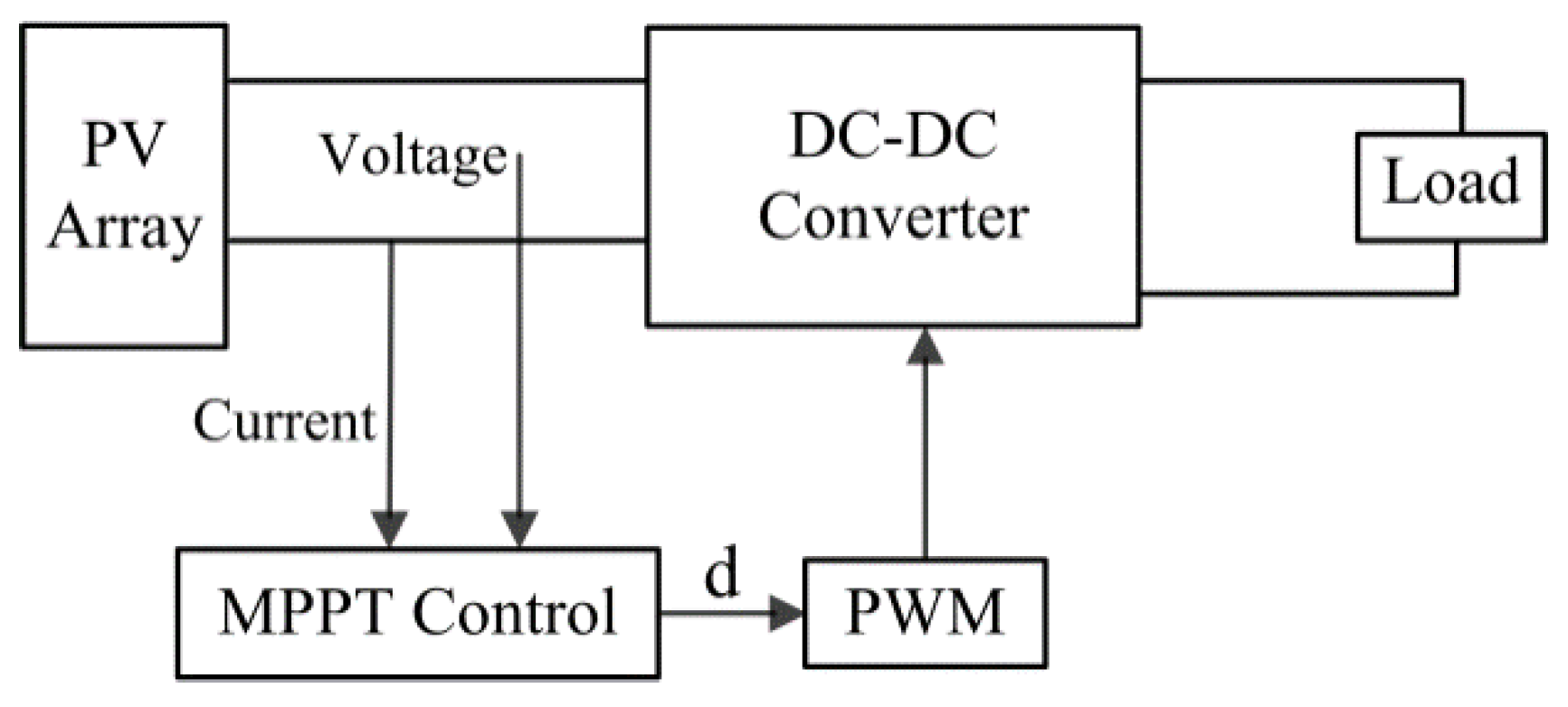
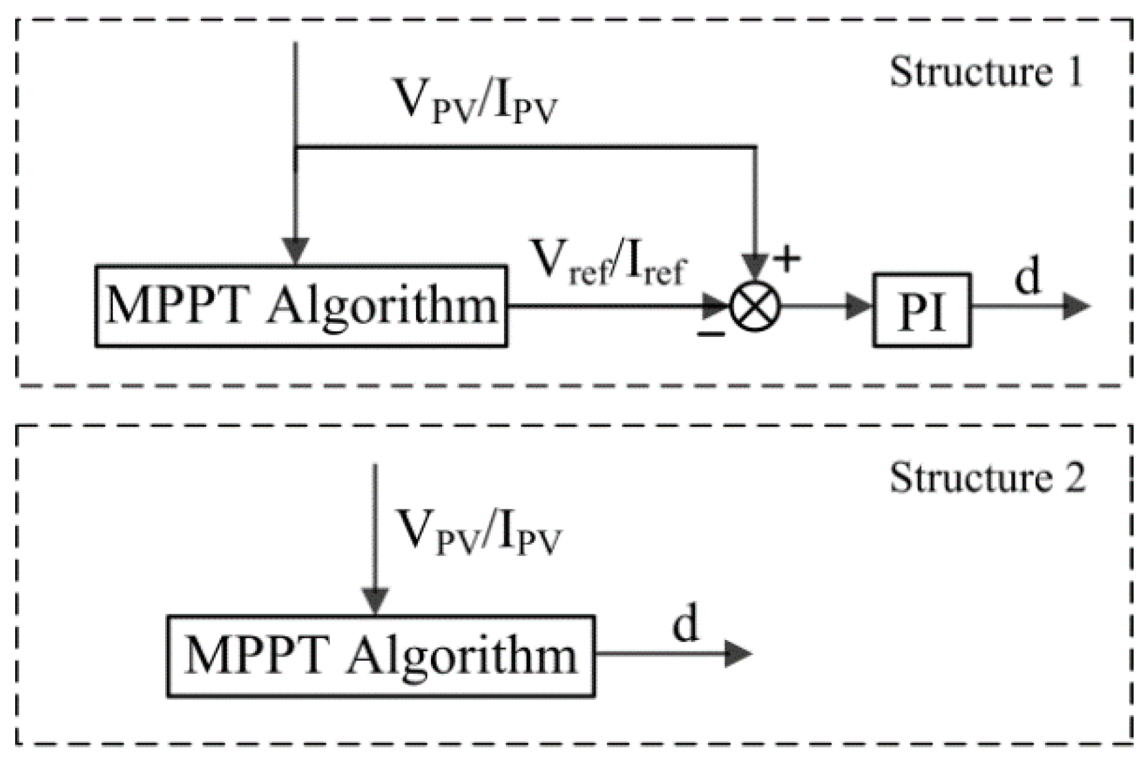
2.2. MPPT Control Unit

According to the output differences of the MPPT algorithm, structures of INC MPPT control unit can be divided into two groups. As shown in Figure 3, the MPPT algorithm generates a reference signal for the outer control loop in structure 1, and the reference signal is either a voltage or a current reference. A comparator is utilized to calculate the error signal of voltage or current, and this error signal is utilized by Proportional Integral (PI) controller to acquire the duty cycle of power converter. Instead of selecting a PV array voltage or current as the output variable, the duty cycle of the power converter is obtained directly by the MPPT algorithm in structure 2, which results in a simplified structure due to the absence of PI controller. However, the additional PI controller leads to a higher efficiency and a faster dynamic performance in structure 1 [10]. The MPPT algorithm will be discussed in detail in Section 3.

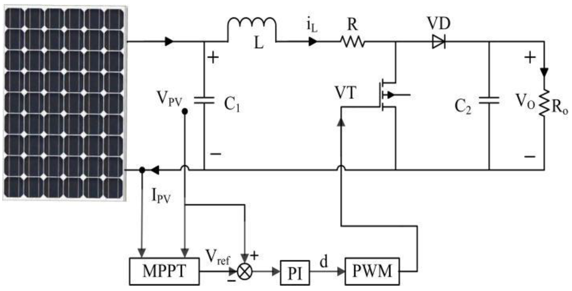
2.3. DC-DC Converter Analysis

Generally, a boost converter is utilized as the power processing unit. As shown in Figure 4, the boost converter consists of an inductor, a diode and two capacitors, as well as a metallic oxide semiconductor field effect transistor (MOSFET) switch.

To design the voltage control loop of the PV system, further studies are needed to analyze how variation in the duty cycle d(t) affects the input voltage V_PV. The state-space averaging method [19] is applied next to derive the low-frequency small-signal model and transfer function for the boost converter.

It is assumed that the boost converter operates in continuous current mode, and the natural frequency of the converter is far less than the switching frequency. The input voltage V_PV, inductor current i_L, and output voltage V_O are chosen as state variables, that is, x = [V_PV(t), i_L(t), V_O(t)]^T. The input variable is input current i_PV, namely u = i_PV(t). Taking output voltage V_O as the output variable, that is, y = V_PV(t). According to KCL (Kirchoff's Current Law) and KVL (Kirchhoff’s Voltage Law), the state equation is given as:

$$\{\begin{array}{l}\stackrel{·}{x}=Ax+Bu\\ y=C^{T}x\end{array},$$

(4)

where $A=d{A}_d+(1-d)A_{1-d}=\left[\begin{array}{ccc}0& -1/C_1& 0\\ 1/L& -R/L& (d-1)/L\\ 0& (1-d)/C_2& -1/R_O{C}_2\end{array}\right]$, $B=\left[\begin{array}{l}1/C_1\\ 0\\ 0\end{array}\right]$, $C=\left[\begin{array}{l}1\\ 0\\ 0\end{array}\right]$.

Introducing small perturbation $(\stackrel{\wedge }{x},\stackrel{\wedge }{u},\stackrel{\wedge }{y},\stackrel{\wedge }{d})$ around the steady state points, and neglecting the quadratic term, the dynamic equation of boost converter is then described as:

$$\{\begin{array}{l}\stackrel{·}{x}=A\stackrel{\wedge }{x}+B\stackrel{\wedge }{u}+E*\stackrel{\wedge }{d}\\ \stackrel{\wedge }{y}=C^T\stackrel{\wedge }{x}\end{array},$$

(5)

where $E=(A_d-A_{1-d})x=\left[\begin{array}{ccc}0& 0& 0\\ 0& 0& 1/L\\ 0& -1/C_2& 0\end{array}\right]\left[\begin{array}{l}{V}_{PV}\\ i_L\\ V_O\end{array}\right]={\left[0V_O/L-i_L/C_2\right]}^T$.

From the Laplace Transform, the state equation becomes:

$$\{\begin{array}{l}(sI-A)\stackrel{\wedge }{x(s)}=B\stackrel{\wedge }{u(s)}+D\stackrel{\wedge }{d(s)}\\ \stackrel{\wedge }{y(s)}=C^T\stackrel{\wedge }{x(s)}\end{array}.$$

(6)

The transfer function of control to PV voltage can be represented as:

$$\begin{array}{lll}{G}_{vd}(s)& =\frac{\stackrel{\wedge }{V_{PV}(s)}}{\stackrel{\wedge }{d(s)}}=\frac{\stackrel{\wedge }{y(s)}}{\stackrel{\wedge }{d(s)}}=C^T{(sT-A)}^{-1}D=\frac{1}{\left|sT-A\right|}\times (-\frac{V_O}{L{C}_1}s-\frac{V_O+R(1-d)i_L}{RL{C}_1{C}_2})& =-\frac{a_{1}s+a_0}{s^3+b_2{s}^2+b_{1}s+b_0}\end{array},$$

(7)

where $a_1=V_o/L{C}_1$, $a_0=\frac{V_o+R_{\mathrm{o}}(1-d)i_L}{R_{o}L{C}_1{C}_2}$, $b_2=\frac{1}{R_o{\mathrm{C}}_2}+\frac{R}{L}$, $b_1=\frac{C_2+C_1{(1-d)}^2}{L{C}_1{C}_2}+\frac{R}{R_{o}L{C}_2}$, and $b_0=1/R_{o}L{C}_1{C}_2$.

3. MPPT Algorithm

3.1. Variable Step Size Method

For fixed step size INC method, a larger step size contributes to a faster response, while more power losses are caused in steady state, thus resulting in a comparatively low efficiency. This situation is the opposite for small step size. Hence, contradiction occurs between the tracking speed and steady state performance. Such a design dilemma can be settled with a variable step size algorithm. The fixed step size is replaced by a function that depends on the derivative of power to voltage (dP/dV), and the algorithm is given by:

$$V_{ref}(k)=V_{ref}(k-1)\pm N\times \left|dP/dV\right|,$$

(8)

where V_ref is the reference voltage, k and k − 1 are the present and previous time interval, N is the scaling factor.

Variable step size methods can also be realized through the slope of P-D curve [20], and the update rule of the MPPT algorithm is presented as:

$$D(k)=D(k-1)\pm N\times \left|dP/dV\right|,$$

(9)

where D(k) is the duty cycle of power converter at time interval k. To guarantee the convergence of the MPPT algorithm, the scaling factor must obey the following inequality [13]:

$$N<\Delta D_{\max }/\left|dP/dV\right|,$$

(10)

where ΔD_max is the upper limiter of step size. If Equation (10) is satisfied, the system will be working in variable step size mode; otherwise, the system will be operating with a fixed step size of ∆D_max.

However, the scaling factor N and the upper limiter of step size ΔD_max cannot be altered once it is tuned at design time. The selection of N and ΔD_max determines which region the working point of the system is located in. An optimal speed factor N failed to satisfy the need of maximum power tracking under the condition of intense irradiation change.

As shown in Figure 5, curve P₁ and P₂ are the output power of a PV array under different irradiation levels. The scaling factor N₁ and upper limiter step size ΔD_max1 are chosen by reference to P₁; in this case, fast dynamic response and good steady performance are achieved simultaneously. However, when irradiation changes greatly, the same parameters always make the system operate within the variable step size mode for P₂ curve, which increases the start-up time, as well as the response time. If the scaling factor N₂ and upper limiter of step size ΔD_max2 are selected according to power curve P₂, the variable step size area of the system that worked for P₁ curve becomes too small, which incurs severe oscillations at steady state and continuous power loss. All in all, the parameters have a significant effect on the system performance, and a poor choice may lead to inefficiency or failure during start-up or dynamic tracking. It is then impossible to find suitable scaling factor and upper limiter of step size that satisfy the requirements of the MPPT system under enormous irradiance changes. Furthermore, manual tuning of these parameters for different kinds of PV arrays restricts its application.

To improve the problem above, an incremental resistance MPPT method is examined with a modified variable step size [14], and a threshold function is introduced to switch the step size modes of the MPPT algorithm:

$$F=P\times \left|dP/dI\right|.$$

(11)

The threshold function F has two extreme points at the two sides of MPP. The system works in the variable step size mode, with a proportionality factor of $\left|dP/dI\right|/\sqrt{1+{\left|dP/dI\right|}^2}$ to adjust the step size when the operating point is located between the two extreme points. Otherwise, it operates in the fixed step size mode. This method automatically adjusts the area of variable step size mode and the step size to track the MPP as irradiation changes. The dynamic speed and steady-state performance are improved as well. However, the value of the threshold function is very large, and, more than once, derivatives are needed to calculate the extreme points as well as the proportionality factor, which generates pretty heavy computational loads. Furthermore, the expression of the proportionality factor is very complex and strong non-linearity exists. MPPT algorithms based on the current-mode feedback control are less stable than the voltage-mode feedback control, especially when irradiation drops sharply [21].

Two step size adjustment coefficients are introduced to eliminate the differences caused by various irradiation levels [15]. The adjustment coefficients are as follows:

$$\{\begin{array}{ll}F\equiv 1-\left|\frac{I}{V_{}}\right|/\left|\frac{dI}{dV}\right|& when\frac{dI}{dV}+\frac{I_{}}{V_{}}<0\\ G\equiv 1-\left|\frac{dI}{dV}\right|/\left|\frac{I_{}}{V_{}}\right|& when\frac{dI}{dV}+\frac{I_{}}{V_{}}<0\end{array}.$$

(12)

This method judges firstly whether the work point is located on the left side or the right side of the MPP and then selects the corresponding formula to calculate. It is based on dI/dV and V/I, which can reduce the computation burden effectively. However, this scheme does not take into consideration that the initial step size has an effect on the performance of the system.

Lastly, a novel concise adaptive variable step size INC algorithm is proposed for the maximum power harvest under the conditions of enormous irradiance changes.

3.2. Proposed Methods

Conventional algorithms of variable step size usually regulate step size through the derivative of power to voltage (dP/dV) of the PV array; however, as shown in Figure 5, derivative curves differ greatly under different irradiation levels. The derivative of power to voltage of PV array is given as:

$$\frac{dP}{dV}=\frac{d(V\times I)}{dV}=I+V\times \frac{dI}{dV}.$$

(13)

Equation (12) indicates that the difference of derivative curves mainly depends on the output current, while output current relies on the irradiation as shown in Equation (3). Hence, a novel adjustment coefficient S(k) is presented to eliminate the difference caused by the output current under various irradiation levels:

$$S(k)=\frac{1}{I}\times \left|\frac{dP}{dV}\right|=\left|1+\frac{V}{I}\times \frac{dI}{dV}\right|,$$

(14)

where V/I represents instantaneous resistance and dI/dV represents incremental conductance. Figure 6 shows that, as output voltage V increases, V/I increases from zero, while dI/dV is almost zero when the operation voltage is located in the left side of MPP, where the current change is almost zero, and dI/dV decreases along with V increases. Therefore, (V/I) × (dI/dV) decreases negatively, and its practical value is −1 at the MPP (curves shown in Figure 6 is normalized value), which can be also validated as follows:

$${\frac{dP}{dV}|}_{MPP}=I+V\times \frac{dI}{dV}=0,$$

(15)

$${\frac{V}{I}\times \frac{dI}{dV}|}_{MPP}=-1.$$

(16)

As shown in Figure 7, S₁ and S₂ are the adjustment coefficient curves corresponding to P₁ and P₂, respectively. Value of the adjustment coefficient S(k) decreases with the operating point getting close to the MPP, and it becomes zero when the system arrives at the MPP. Change trends and value ranges of S(k) are roughly the same under different irradiation levels. Furthermore, compared with the dP/dV, the adjustment coefficient S(k) varies more smoothly since its value is relatively smaller. Therefore, the adjustment coefficient S(k) is better suited for regulating the step size to track the MPP.

It should be noted that the adjustment coefficient S(k) rises rapidly on the right hand side of the MPP, which may incur instability of MPPT algorithm. Hence, S(k) must meet the following inequality on the right hand side of the MPP: S(k) ≤ 1. Figure 7 shows the normalized S(k) without regulation, and the practical curves of S(k) with constraint are illustrated in Figure 8. Value of the adjustment coefficient S(k) stays at 1 when the operating point is far away from the MPP, and decreases with the operating point getting close to the MPP.

The update rule of the improved variable step size INC algorithm is thus obtained as:

$$V_{ref}(k)=V_{ref}(k-1)\pm \mathrm{S}(k)\times \Delta V_{ref},$$

(17)

where V_ref(k) is the reference voltage at time k, V_ref(k − 1) is the reference voltage at time k − 1, and ΔV_ref(k) stands for the initial perturbation step size.

The flowchart of the proposed method is shown in Figure 9, the fundamental INC strategy is used to judge whether the operating point is located on the right or left hand side of the MPP. When the system operates on the right hand side of the MPP and S(k) ≥ 1, the proposed method is forced to operate in fixed step mode with step size ΔV_ref. Otherwise, it operates in variable step size mode with step size S(k) × ΔV_ref. The proposed method provides a simple and effective way to harvest the maximum power.

Study of P-V curves suggests that PV characteristics display a significant difference near the MPP. The output power curve varies smoothly on the left hand side of the MPP, while it ascends sharply on the right hand side. This feature can be applied for MPPT to further improve the dynamic response and steady output. The initial perturbation step size ΔV_ref(k) is represented as:

$$\Delta V_{ref}=\{\begin{array}{ll}\Delta V_{ref1}& 0<V<V_{MPP}\\ \Delta V_{ref2}& V_{MPP}<V<V_{OC}\end{array},$$

(18)

where ΔV_ref1 and ΔV_ref2 are initially selected as the upper limit for the variable step size mode, ΔV_ref1 operates on the left hand side of the MPP, and ΔV_ref2 operates on the right hand side. The relationship between ΔV_ref1 and ΔV_ref2 can be expressed as:

$$\frac{\Delta V_{ref1}}{\Delta V_{ref2}}=\frac{V_{MPP}}{V_{OC}-V_{MPP}},$$

(19)

where V_MPP and V_OC are the PV array voltages corresponding to MPP and open circuit, respectively.

According to the FOV [4] method, the relationship between V_MPP and V_OC of a PV array is close to linear under various atmospheric conditions:

$$V_{MPP}\approx \mathsf{\mu }{V}_{OC},$$

(20)

where μ is a proportionality constant, and its value lies between 0.71 and 0.78 [21]. Thus,

$$\frac{\Delta V_{ref1}}{\Delta V_{ref2}}=\frac{\mathsf{\mu }}{1-\mathsf{\mu }}.$$

(21)

In this paper, μ is set as 0.75, therefore ΔV_ref1 = 3 × ΔV_ref2.

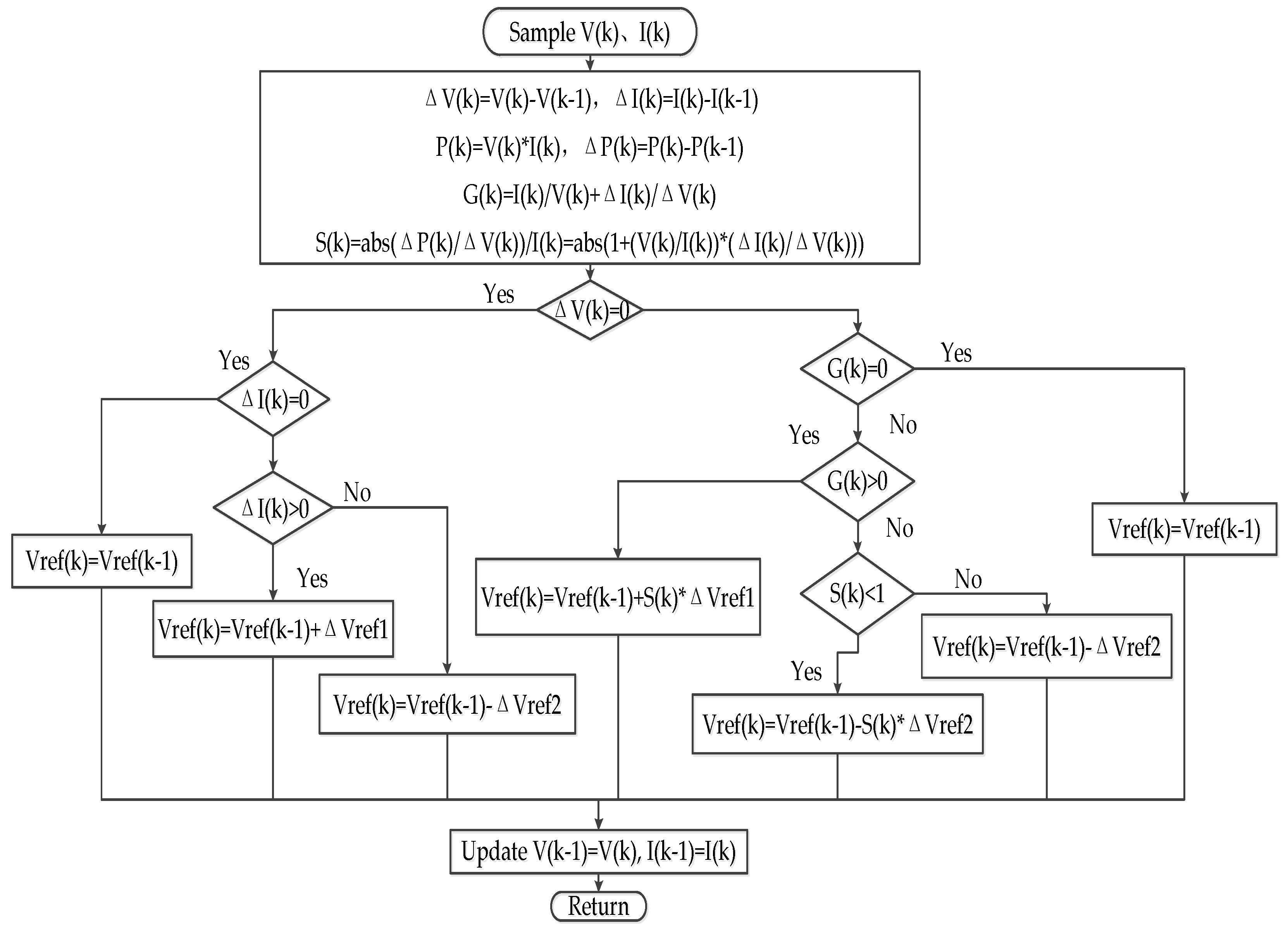
3.3. Realization of the Proposed Algorithm

The voltage control loop is implemented through a PI controller, and the transfer function of the PI controller is obtained as:

$$G_c(s)=K_p+K_i/s.$$

(22)

The PI controller gains are designed with the small signal model transfer function G_vd(s); thus, the open loop transfer function is expressed as:

$$G_o(s)=G_{vd}(s)G_c(s).$$

(23)

Parameters of PV array and boost converter are shown in

Table 1. Parameters of photovoltaic (PV) array and boost converter.

PV Parameters	Value
Open-circuit Voltage VOC	300 V
Short-circuit Current ISC	0.9 A
Voltage at the MPP VMPP	223 V
Current at the MPP IMPP	0.8 A
Maximum Power P	178.4 W
Input Filter Conductor C1	165 μF
Filter Inductor L	1 mH
Inductor Resistance R	0.052 Ω
Output Filter Conductor C2	2500 μF
Switching Frequency f	20 kHz

. Substituting relevant variables into Equations (19) and (20), the bode plot of G_o(s) with compensator and without compensator is obtained, as shown in Figure 10. From the plots, it is observed that phase margin, cutoff frequency and magnitude margin without compensator is −179°, 3.5 krad/s, and −45.4 dB, respectively. Phase margin is required to be greater than 30°, magnitude margin should be more than 6 dB. Therefore, parameters of PI controller are derived as K_p = 0.107, K_i = 346.5. Phase margin, cutoff frequency and magnitude margin with compensator is 119°, 1.71 krad/s, and infinity, respectively. Obviously, a close loop system has good stability due to the PI compensator. Figure 11 shows the step response of a voltage close loop with PI controller. The fast response is validated by the rise time of 0.0028 s and the settling time of 0.012 s.

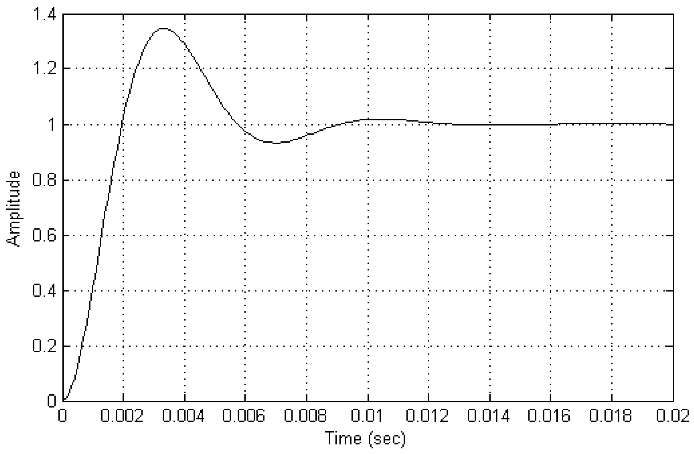
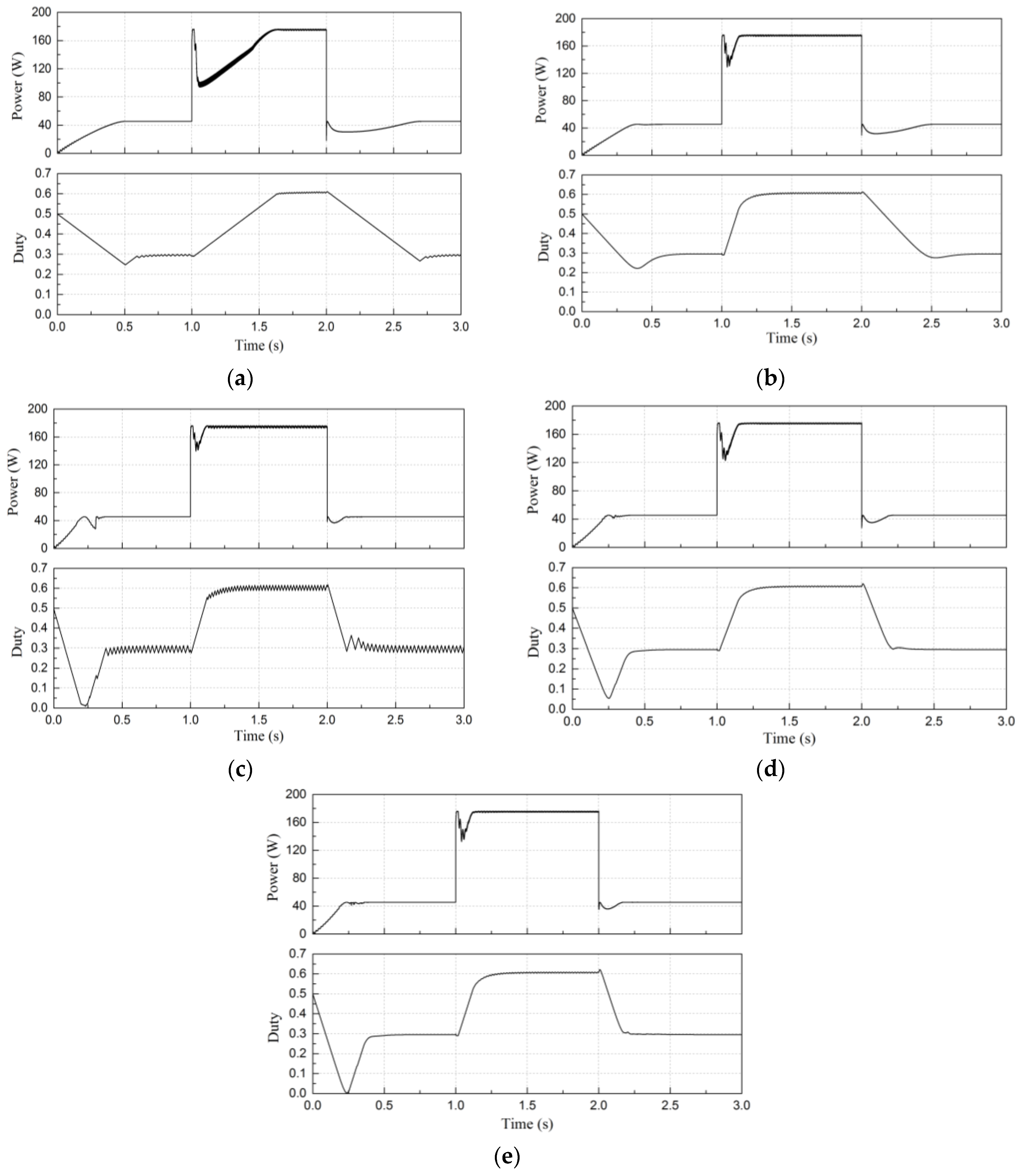
4. Simulation Analysis

As illustrated in Figure 4, a simulation model of PV system is developed in Matlab/Simulink to verify the effectiveness of the proposed algorithm. To compare the performance of the MPPT methods, a series of simulations are conducted under the same step-change of irradiation conditions, from 300 to 1000 W/m² at 1.0 s and back to 300 W/m² at 2.0 s. Simulation waveforms of PV output power and duty cycle of MPPT are presented in Figure 12. Figure 12a,b are traditional INC methods with fixed step size, and Figure 12c is a typical representative variable step size INC method [13], which is easy to implement with good tracking speed and stability performance, relatively. Figure 12d,e are proposed methods with different initial step sizes.

Table 2. Comparison of different maximum power point tracking (MPPT) methods.

Method	Parameters	Tracking Time with Irradiation Step Change			Average Power at 1000 W/m2
		0 to 300 W/m2	300 to 1000 W/m2	1000 to 300 W/m2
Fixed step size	ΔVref = 1 V	0.56 s	0.65 s	0.70 s	175.5 W
	ΔVref = 4.8 V	0.37 s	0.13 s	0.16 s	172.6 W
Variable step size	N = 1, ΔVrefmax = 4.8 V	0.55 s	0.22 s	0.51 s	175.4 W
Proposed method	ΔVref1 = ΔVref2 = 4.8 V	0.39 s	0.16 s	0.204 s	175.4 W
	ΔVref1 = 4.8 V, ΔVref2 = 1.6 V	0.38 s	0.14 s	0.165 s	175.6 W

provides comparison details of different MPPT methods.

Figure 12a,b show the INC method with fixed step size of 1 and 4.8 V, respectively. It is observed that the tracking time with fixed step size of 4.8 V is 0.13 and 0.16 s, which is shortened by 0.52 and 0.54 s than the fixed step size of 1 V. However, the average output power of PV array is decreased from 175.5 to 172.6 W at 1000 W/m². It indicates that larger step size significantly improves the response time, but more power loss is incurred due to the steady state oscillation of the converter duty cycle.

Results of variable step size INC are illustrated in Figure 12c. As the scaling factor N is set as 1 and the upper limit of step size ΔV_refmax is set as 4.8 V in [13] and experiments show that the parameters can ensure the system to maintain a good performance when irradiance change is not so large, this paper chooses N = 1 and ΔV_refmax = 4.8 in Figure 12c for reference. Compared with the fixed step size INC method, the variable step size method partly solves the contradiction between the response speed and steady state performance. The duty cycle oscillation is very small around the steady state; therefore, the average output power of PV array is 175.4 W at 1000 W/m², and the tracking time of 300 to 1000 W/m² is 0.22 s. However, the start-up time and tracking time of irradiation drop is a little long about 0.55 and 0.51 s, respectively.

For the proposed variable step size method, both the fixed step size ΔV_ref1 and ΔV_ref2 are set as 4.8 V, and the corresponding results are shown in Figure 12d. Figure 12e illustrates the proposed MPPT method with different fixed step sizes (ΔV_ref1 = 4.8 V, ΔV_ref2 = 1.6 V), which also satisfies Equation (20). Compared with the traditional variable step size INC method, start-up time of the proposed method with equal step size is reduced from 0.55 to 0.39 s, and the tracking time under irradiation change condition is also shortened by 0.06 s and 0.31 s. It also can be seen that the proposed algorithm with different initial step sizes in Figure 12e has a better dynamic performance than that of the proposed algorithm with the same initial step size in Figure 12d, while the steady-state oscillations almost have no difference. These results suggest that the proposed method can achieve fast dynamic response and stable output power simultaneously even under the enormous irradiation change conditions.

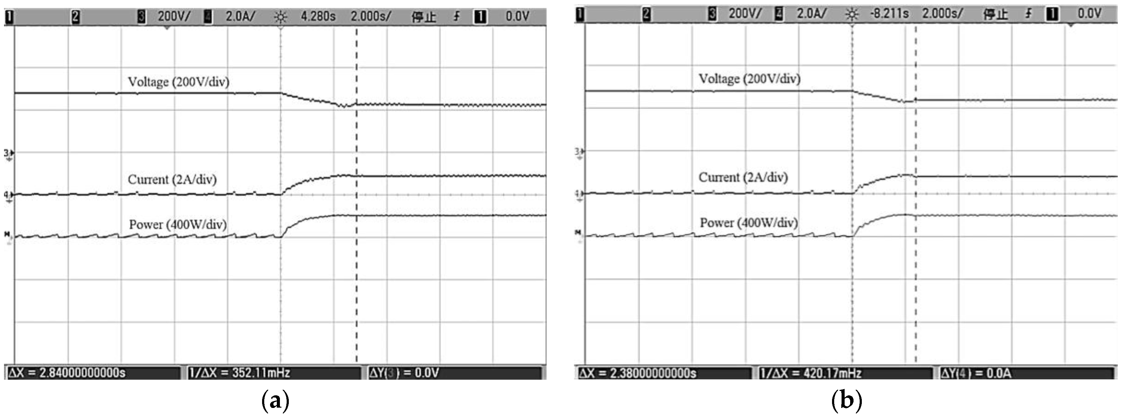
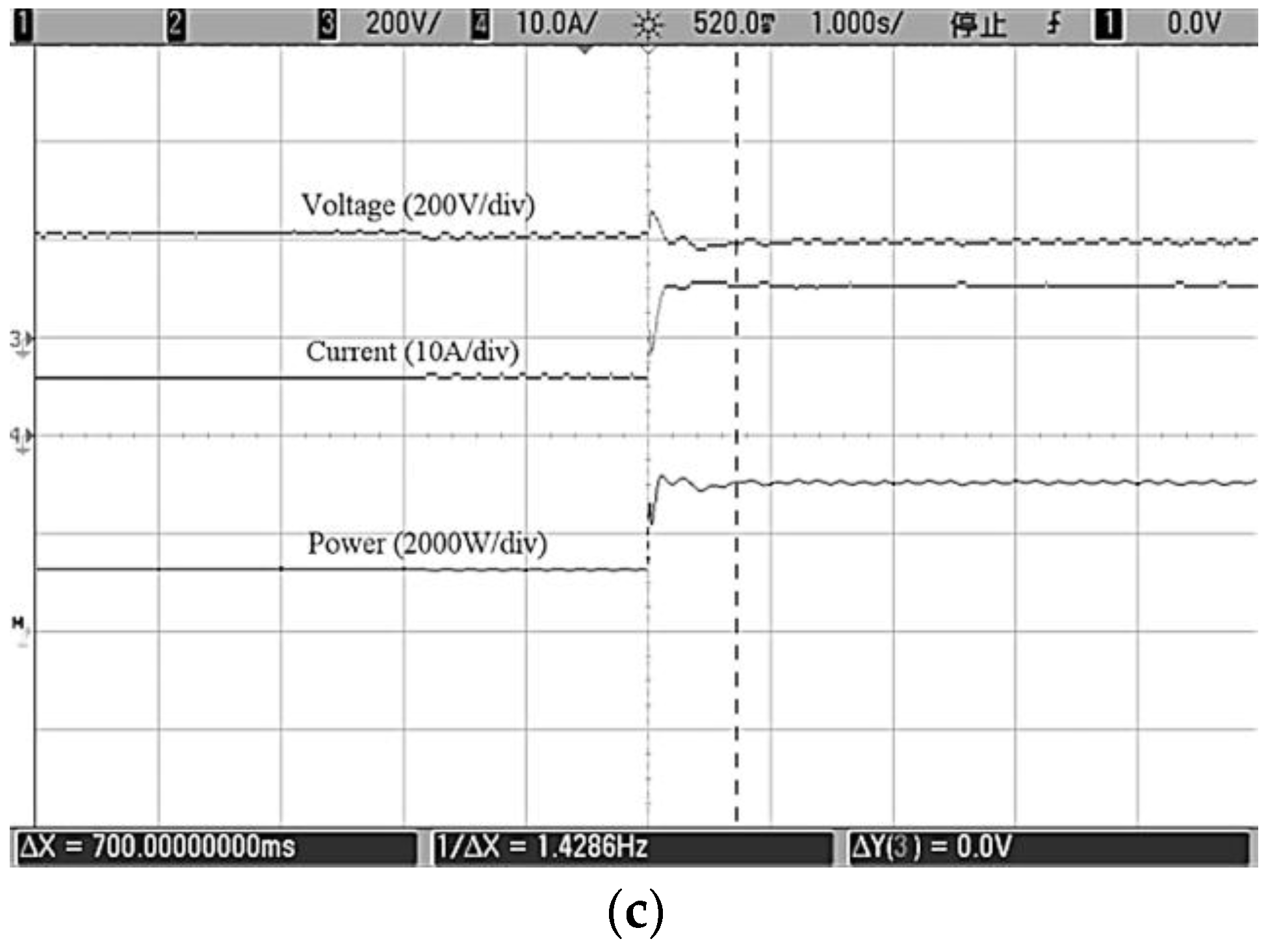
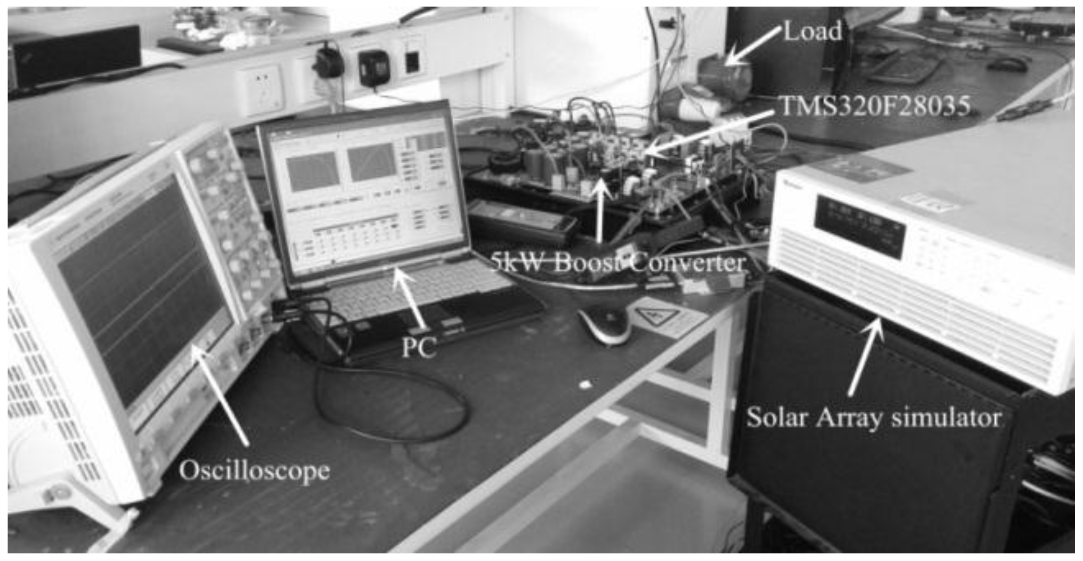
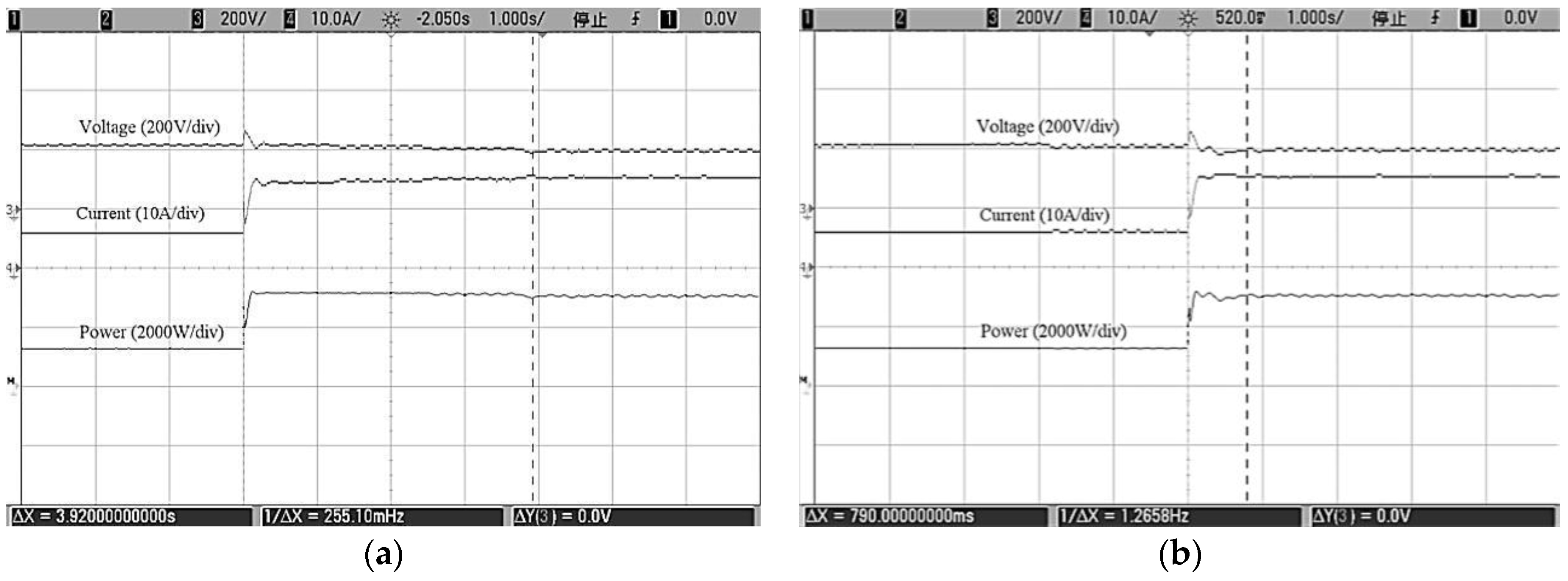
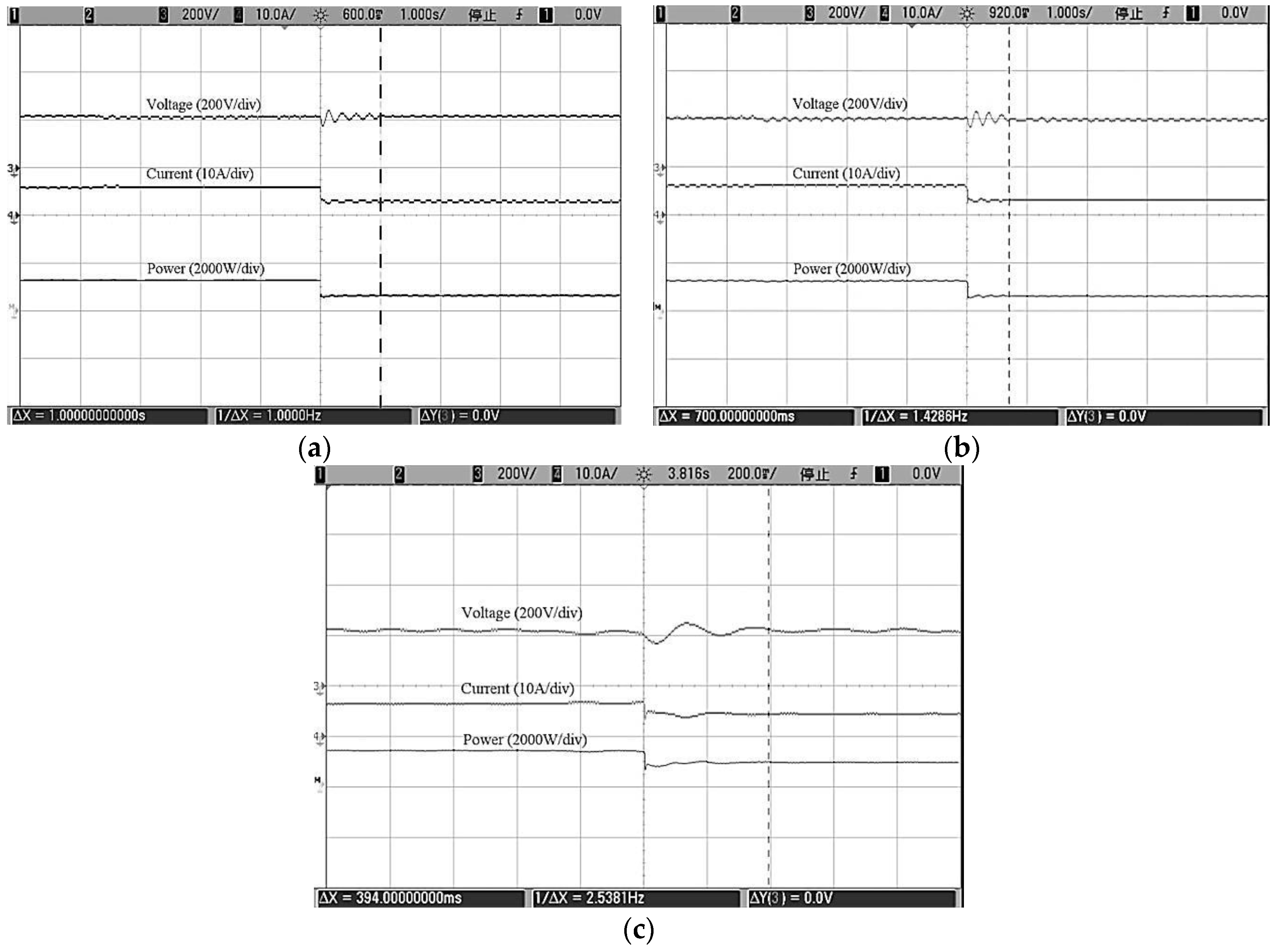
5. Experiment Results

To verify the effectiveness of the proposed algorithm, an experimental prototype is established as shown in Figure 13. A programmable DC power supply (Solar Array Simulator Chroma 6200H) (Chroma, Shenzhen, China) is used to simulate the output characteristics of PV arrays and a 5 kW boost converter is implemented as the power interface between the PV array and the load. At present, 5 kW is widely used in the actual photovoltaic system, and using 5 kW PV system to verify the proposed algorithm has very good practical significance. The MPPT algorithm is realized in CCS (Code Composer Studio) IDE (integrated development environment) (TEXAS INSTRUMENTS, Shenzhen, China), is then downloaded onto a digital signal controller TMS320F28035 (TEXAS INSTRUMENTS, Shenzhen, China). Parameters of the PV array and boost converter are illustrated in Table 1.

Three INC MPPT algorithms are tested in the same experimental conditions to analyze the performance of the proposed method:

• Traditional variable step size INC: N = 1, ΔV_refmax = 4.8 V.
• Proposed method with equal initial step sizes: ΔV_ref1 = ΔV_ref2 = 4.8 V.
• Propose method with initial step sizes that satisfy Equation (20): ΔV_ref1 = 4.8 V, ΔV_ref2 = 1.6 V.

In order to compare the start-up performance of traditional variable step size INC and the proposed method, corresponding experiments are conducted by regulating parameters of the PV array simulator. Based on the principle of convenient observation for tracking time and tracking precision, the resolution of voltage, current and power is selected, respectively, as Figure 14, Figure 15 and Figure 16.

Figure 14a shows the start-up waveforms of variable step size INC, and it takes 2.84 s to reach the MPP. It can be seen from Figure 14b that the start-up time of the proposed method with equal initial step sizes is 0.46 s faster than the traditional variable step size INC with only 2.38 s. Furthermore, compared with the traditional variable step size INC, the oscillations at steady state are reduced for the proposed method. Waveforms of the proposed method with different initial step sizes are almost the same as Figure 14b. The results suggest that the proposed MPPT method keeps a larger step size than traditional variable step size INC in the start-up process, thus improving the start-up performance of MPPT method. In addition, steady state oscillations are reduced because the adjustment coefficient S(k) adopted by proposed method varies more smoothly.

Dynamic tracking experiments are also conducted to compare the tracking performance of MPPT methods. The rise-up situation can be simulated by increasing the output power of the solar array simulator, and the output waveforms of PV array are presented in Figure 15. Figure 15a shows the results of the traditional variable step size INC, and it takes 3.92 s to reach the MPP. As can be seen from Figure 15b,c, tracking time of the proposed method with equal initial step sizes and different initial step sizes is 0.79 and 0.7 s, respectively. It is obvious that the proposed method obtains a faster response than the traditional variable step size INC method when irradiation rises suddenly.

In the same way, the decreasing situation can be simulated by decreasing the output power of the solar array simulator. Traditional variable step size tracks the MPP within 1.0 s in Figure 16a. Figure 16b shows the results of the proposed MPPT method with equal initial step sizes, and the tracking time is 0.3 s faster than the traditional variable step size INC. Meanwhile, it takes 0.394 s for the proposed MPPT method with different initial step sizes to reach the MPP in Figure 16c, thus further improving the tracking speed.

These experimental results provide substantial evidence for the theoretical assumption that the proposed MPPT method performs a faster dynamic response than traditional variable step size INC methods under the sudden changes of irradiation conditions, as well as a better steady state performance. In addition, as affected by the control period, the sampling precision, and the disturbance step, it is a normal phenomenon that oscillation exists in the voltage and current waveforms of experimental results.

6. Conclusions

In this paper, a novel INC MPPT algorithm is proposed with adaptive variable step size. The step size can be automatically regulated to track MPP using an adjustment coefficient of step size. The fast response and better steady state performance both are achieved simultaneously even under the condition of enormous irradiance changes. Initial step sizes are well tuned based on the FOV method to further improve the MPPT performance, and this initial step size strategy is also available for other MPPT algorithms. Compared with other INC MPPT methods, the proposed method provides an effective way for maximum power harvest with simple implementation. The results of simulations and experiments further validate the effectiveness and feasibility of the proposed algorithm.

References

1. Kwon, J.M.; Nam, K.H.; Kwon, B.H. Photovoltaic power conditioning system with line connection. IEEE Trans. Ind. Electron. 2006, 53, 1048–1054. [Google Scholar] [CrossRef]
2. Chao, K.H. A high performance PSO-based global MPP tracker for a PV power generation system. Energies 2015, 8, 6841–6858. [Google Scholar] [CrossRef]
3. Esram, T.; Chapman, P.L. Comparison of photovoltaic array maximum power point tracking techniques. IEEE Trans. Energy Convers. 2007, 22, 439–449. [Google Scholar] [CrossRef]
4. Sivakumar, P.; Kader, A.A.; Kaliavaradhan, Y.; Arutchelvi, M. Analysis and enhancement of PV efficiency with incremental conductance MPPT technique under non-linear loading conditions. Renew. Energy 2015, 81, 543–550. [Google Scholar] [CrossRef]
5. Kollimalla, S.K.; Mishra, M.K. A novel adaptive P&O MPPT algorithm considering sudden changes in the irradiance. IEEE Trans. Energy Convers. 2014, 29, 602–610. [Google Scholar]
6. Abdelsalam, A.K.; Massoud, A.M.; Ahmed, S.; Enjeti, P.N. High-performance adaptive perturb and observe MPPT technique for photovoltaic-based microgrids. IEEE Trans. Power Electron. 2011, 26, 1010–1021. [Google Scholar] [CrossRef]
7. Piegari, L.; Rizzo, R.; Spina, I.; Tricoli, P. Optimized adaptive perturb and observe maximum power point tracking control for photovoltaic generation. Energies 2015, 8, 3418–3436. [Google Scholar] [CrossRef]
8. Petrone, G.; Spagnuolo, G.; Teodorescu, R.; Veerachary, M.; Vitelli, M. Reliability issues in photovoltaic power processing systems. IEEE Trans. Ind. Electron. 2008, 55, 2569–2580. [Google Scholar] [CrossRef]
9. Cheng, P.C.; Peng, B.R.; Liu, Y.H.; Cheng, Y.S.; Huang, J.W. Optimization of a fuzzy-logic-control-based MPPT algorithm using the particle swarm optimization technique. Energies 2015, 8, 5338–5360. [Google Scholar] [CrossRef]
10. Mamarelis, E.; Petrone, G.; Spagnuolo, G. Design of a sliding-mode-controlled SEPIC for PV MPPT applications. IEEE Trans. Ind. Electron. 2014, 61, 3387–3398. [Google Scholar] [CrossRef]
11. Ruddin, S.; Karatepe, E.; Hiyama, T. Artificial neural network-polar coordinated fuzzy controller based maximum power point tracking control under partially shaded conditions. IET Renew. Power Gener. 2009, 3, 239–253. [Google Scholar]
12. Pandey, A.; Dasgupta, N.; Mukerjee, A.K. High-performance algorithms for drift avoidance and fast tracking in solar MPPT system. IEEE Trans. Energy Convers. 2008, 23, 681–689. [Google Scholar] [CrossRef]
13. Liu, F.; Duan, S.; Liu, F.; Liu, B.; Kang, Y. A variable step size INC MPPT method for PV systems. IEEE Trans. Ind. Electron. 2008, 55, 2622–2628. [Google Scholar]
14. Mei, Q.; Shan, M.; Liu, L.; Guerrero, J.M. A novel improved variable step-size incremental-resistance MPPT method for PV systems. IEEE Trans. Ind. Electron. 2011, 58, 2427–2434. [Google Scholar] [CrossRef]
15. Chen, Y.; Lai, Z.; Liang, R. A novel auto-scaling variable step-size MPPT method for a PV system. Sol. Energy 2014, 102, 247–256. [Google Scholar] [CrossRef]
16. Faraji, R.; Rouholamini, A.; Naji, H.R.; Fadaeinedjad, R.; Chavoshian, M.R. FPGA-based real time incremental conductance maximum power point tracking ccontroller for photovoltaic systems. IET Power Electron. 2014, 7, 1294–1304. [Google Scholar] [CrossRef]
17. Tey, K.S.; Mekhilef, S. Modified incremental conductance MPPT algorithm to mitigate inaccurate responses under fast-changing solar irradiation level. Sol. Energy 2014, 101, 333–342. [Google Scholar] [CrossRef]
18. Elgendy, M.A.; Zahawi, B.; Atkinson, D.J. Assessment of the incremental conductance maximum power point tracking algorithm. IEEE Trans. Sustain. Energy 2013, 4, 108–117. [Google Scholar] [CrossRef]
19. Erickson, R.W.; Maksimovic, D. Fundamentals of Power Electronics; Springer: Berlin, Germany, 2001. [Google Scholar]
20. Xiao, W.; Dunford, W.G. A modified adaptive hill climbing MPPT method for photovoltaic power systems. In Proceedings of the IEEE 35th Annual Power Electronics Specialists Conference, Aachen, Germany, 20–25 June 2004; Volume 3, pp. 1957–1963.
21. Femia, N.; Petrone, G.; Spagnuolo, G.; Vitelli, M. Power Electronics and Control Techniques for Maximum Energy Harvesting in Photovoltaic Systems; CRC Press: Boca Raton, FL, USA, 2013. [Google Scholar]
Figure 1. Diagram of the photovoltaic (PV) system.
Energies 09 00288 g001
Figure 2. Equivalent circuit of PV array.
Energies 09 00288 g002
Figure 3. Diagram of incremental conductance (INC) maximum power point tracking (MPPT) control unit.
Energies 09 00288 g003
Figure 4. The proposed maximum power point tracking (MPPT) system.
Energies 09 00288 g004
Figure 5. Normalized power, abs(dP/dV) under different irradiation levels.
Energies 09 00288 g005
Figure 6. Normalized V/I, dI/dV and (V/I) × (dI/dV) (p.u.).
Energies 09 00288 g006
Figure 7. Normalized power, abs(dP/dV) and S(k).
Energies 09 00288 g007
Figure 8. Adjustment coefficient S(k) versus voltage.
Energies 09 00288 g008
Figure 9. Flowchart of the proposed algorithm.
Energies 09 00288 g009
Figure 10. Bode plot of voltage control loop.
Energies 09 00288 g010
Figure 11. Step response of voltage control loop with proportional integral (PI) compensator.
Energies 09 00288 g011
Figure 12. (a) Simulation results of fixed step size INC (ΔVref = 1 V); (b) Simulation results of fixed step size INC (ΔVref = 4.8 V); (c) Simulation results of variable step size INC (N = 1, ΔVrefmax = 4.8 V); (d) Simulation results of proposed method (ΔVref1 = ΔVref2 = 4.8 V); (e) Simulation results of proposed method (ΔVref1 = 4.8 V, ΔVref2 = 1.6 V).
Energies 09 00288 g012
Figure 13. The experimental setup.
Energies 09 00288 g013
Figure 14. The start-up waveforms of INC methods (Time (2 s/div)) (a) Variable step size INC; (b) Proposed method (ΔVref1 = ΔVref2).
Energies 09 00288 g014
Figure 15. The rise-up situation (Time (1 s/div)) (a) Variable step size INC; (b) Proposed method (ΔVref1 = ΔVref2); (c) Proposed method (ΔVref1 = 3 × ΔVref2).
Energies 09 00288 g015aEnergies 09 00288 g015b
Figure 16. The decreasing situation (Time (1 s/div)). (a) Variable step size INC; (b) Proposed method (ΔVref1 = ΔVref2); (c) Proposed method (ΔVref1 = 3 × ΔVref2).
Energies 09 00288 g016