Load Concentration Factor Based Analytical Method for Optimal Placement of Multiple Distribution Generators for Loss Minimization and Voltage Profile Improvement

Abstract

This paper presents novel separate methods for finding optimal locations, sizes of multiple distributed generators (DGs) simultaneously and operational power factor in order to minimize power loss and improve the voltage profile in the distribution system. A load concentration factor (LCF) is introduced to select the optimal location(s) for DG placement. Exact loss formula based analytical expressions are derived for calculating the optimal sizes of any number of DGs simultaneously. Since neither optimizing the location nor optimizing the size is done iteratively, like existing methods do, the simulation time is reduced considerably. The exhaustive method is used to find the operational power factor, and it is shown with the results that the losses are further reduced and voltage profile is improved by operating the DGs at operational power factor. Results for power loss reduction and voltage profile improvement in IEEE 37 and 119 node radial distribution systems are presented and compared with the the loss sensitivity factor (LSF) method, improved analytical (IA) and exhaustive load flow method (ELF). The comparison for operational power factor and other power factors is also presented.

1. Introduction

Distributed, renewable Generation (DGs) in conventional power systems have received increased interest in research over the last decade due to its environmentally friendly nature and potential economic benefits. The integration of DG(s) becomes the most economical solution to meet the increased demand due to load growth in the conventional system [1]. Technological advancements in generators, power electronics devices and storage devices further fuel this trend. DGs contribute in the application of competitive energy policies, diversification of energy resources, reduction of on-peak operating cost, deferral of network upgrades, lower losses and lower transmission and distribution costs, and potential increase of service quality to the end-customer [2].

Based on the technologies used for DGs, these can be either renewable based or nonrenewable based, both having their own advantages and disadvantages. The former being environmentally friendly is the preferable choice but these have a disadvantage of low efficiency, high costs and intermittency because these technologies are not matured enough. Improvement in efficiency and reduction in cost is expected in the future due to technological developments and new scientific methods of designing [3]. Nonrenewable based DGs, e.g., internal combustion engines or combustion turbines etc., are relatively more efficient but are not as environmentally friendly [4,5]. For geothermal, small hydro, and combined cycles, combustion and wind turbines with power electronics, DGs are considered as synchronous generators. Moreover, DGs are modeled as power electronic converters or static generators for photovoltaic (PV) or fuel cell based plants and droop-control based techniques are used for control (decentralised) of such DGs, as presented in [6,7,8].

While providing environmentally friendly energy and while helping to meet the increasing load economically, DGs are also proven to be beneficial in providing reduction in power losses, improving voltage profile, and improving the power handling capability and power quality of the system. Such benefits can only be exploited when the location and size of the DG(s) are properly chosen. Voltage and loadability enhancement, reliability improvement and network upgrade deferral are also influenced by the location and sizing of DGs [9]. Similarly, DGs have been integrated in electricity markets for ancillary services such as spinning reserve, reactive power support, loss compensation, frequency control and other fast response services. On the other hand, poorly planned and improperly operated DG units can lead to reverse power flows, excessive power losses and overheating of feeders [10]. Reverse power flow may be a problem because the conventional controlling schemes and operational procedures assume unidirectional power flow and hence bidirectional (reverse) power flow can lead to adverse impact on them [11]. Reverse power flow can create problems such as voltage rise in distribution grids, leading to the violation of the requirements set in standard EN50160 [12]. Short circuit currents increased to the damaging levels, protection desensitization and incorrect operation of control equipment are some other expected problems due to reverse power flow [13]. The proposed method also works when reverse power flow is allowed and handled properly in the system. In order to achieve one or several of the aforementioned benefits, location and size of DG(s) have to be optimized. To get maximum advantages, this problem is usually approached by splitting it into two parts, finding the optimum location and then sizing the DG at this optimum location [14].

When considering the current scenario of DG penetration, it can be referred to as the “popping up like mushrooms” situation because the investors can make studies on their own economic benefits and primary energy availability for installing a DG. If they abide by certain grid codes, these DGs must be connected to the system. Unfortunately, there are no detailed considerations of reducing power losses and other technical aspects that might support the consumer or distribution network operator (DNO). The major motivation behind this study is to investigate the impact of a situation which is contrary to the current scenario i.e., to provide the DNO with a certain level of control for steering up the direction of DG penetration. In the current situation, loss reduction is not considered. It is expected that the DNO will identify the location(s) and the desired generation patterns from DGs so that the system performance is improved and the grid reinforcements can be deferred. The proposed study tries to justify the need of giving a DNO some control over DG installation based on system improvements. As this is not in line with the current practice due to unbundling rules, keeping in view the potential benefits, the DNO can offer benefits to the investors to install DGs of desired sizes at studied locations. Offering benefits to the investors can be justified against the economic benefits a DNO gets because of reduction of cost for improving voltage profile and, maybe, saving because of reduced losses.

The authors in [15] have obtained the optimal location and size for real power loss reduction to place a single DG. The importance of selecting the correct DG size and location is also shown. It is also agreed that real constraints may also be considered for choosing the location for DG placement, but, once the location is selected, the optimum size should not be compromised to get maximum benefits. Authors in [16] have proved the impact of DG location and sizing for different loading conditions and showed that the losses also depend on the loading conditions. The impact of DGs on load supply cost has been discussed in [17], which uses evolutionary programming (EP). The high losses index has been utilized to improve the performance of the proposed algorithm. Reference [18] proposed a particle swarm optimization (PSO) based technique for optimal DG placement and sizing. Along with reduction in real power losses, impact of various load models and technical issues such as power factor, voltage profile, line loading and total power intake from grid have also been discussed. The local PSO based method for optimal sitting of DGs in order to minimize losses in networks with reverse power flow is discussed in [19]. Optimal sitting is advantageous as it gives the DG sizes and location in such a way that the load is fed locally.

To address the issue of optimum location and size separately, the use of suitable optimization techniques for each part is also used. Diversification of optimization variables and hence the improvement in results are the main advantages expected from such approaches. To get the maximum out of such approaches, the selection of suitable methods for the respective part of the problem is important. For example, the authors in [20] have applied genetic algorithm (GA) for selecting the optimum bus, as it is an integer-based optimization algorithm while, for optimizing the size of DG at given candidate locations provided by GA, PSO is used. Despite being good in meeting the desired performance, it is noteworthy that such approaches are time consuming compared to the case where single optimization is applied throughout. Another such approach is presented in [21] where authors have used Discrete PSO and GA, but these were not used individually for each sub-part. Instead, both algorithms have been mixed, where GA is used for mutation and crossover to eliminate the chances of getting stuck at local minimum. A few other examples of recent research include Kalman filter algorithm [22], EP [23], chance constrained programming [24] and PSO [25].

Along with heuristic and meta-heuristic methods, there has been various research about finding the optimum sizes and location analytically. In [20], the optimal location of a single DG with unity power factor has been done for radial as well as meshed networks. This study is performed with the objective of loss minimization, but the optimum size is not considered. Reference [26] presents an analytical approach based on exact loss formula for optimizing the size and location of DG. This is a considerably fast method but with a disadvantage that it can only compute the size of single a DG capable of delivering real power only. This problem is addressed in [27] where the optimum size of a DG capable of delivering both active and reactive power, and the optimal power factor of individual DGs at optimum location has been calculated. This work is extended for placing multiple DGs in [28], where an iterative procedure is used to select the optimum bus in the system. Despite being able to find the exact size, using iterative methods for finding the optimum location makes this approach slower. Another important point in this method is that it neglects the impact of oncoming generators when calculating the size of a DG. This avoids the method from finding the best solution because it does not include the variations of loss coefficients (alpha and beta in exact loss formula) [29]. In addition, in iterative techniques, the sizes of oncoming DG(s) are calculated based on the already installed DG(s), which limits the range for the optimal sizes of the oncoming DGs. A recent example of analytical method based optimal sitting is discussed in [30] where loss minimization is done by reducing the line currents after placing DGs at various locations. Moreover, based on the found optimal sizes, the combination of DG types is also suggested.

The uncertainties of the DGs can also be considered for optimum locations and sizing as they introduce disturbances in the power networks in terms of large current transients, voltage fluctuations, waveform distortions, and long voltage variation etc. In [31], three step GA and decision theory based procedure is proposed to obtain best generation size and location for DG considering unavoidable uncertainties. A robust planning methodology to improve the accuracy of Monte Carlo simulations nested in an evolutionary algorithm is formulated in [32] to assess the trade-offs in technical and economic aspects. Genetic algorithm embedded with point estimate method (GA-PEM) based approach has been proposed for solving optimization problem of probabilistic power flow (PPF) modeled uncertainty under chance constrained programming for non-deterministic load growth and nondispatchable renewable resources in [33]. A Monte Carlo simulation-embedded genetic-algorithm-based approach is employed in [24] for optimally sitting and sizing of DGs. The chance constrained programming (CCP) model is developed of cost minimization with security limitations as constraints, considering uncertainty of stochastic power production.

For choosing the optimum bus number, various methods have been explored. Loss sensitivity factor (LSF), exhaustive load flow (ELF), improved analytical (IA) method, which is an iterative technique, gradient and second order methods, and GA based selection of optimum location(s) are just a few methods for choosing optimum locations in order to reduce losses [27,28,34]. All these methods provide the location selection as a builtin feature; therefore, one needs to implement a whole algorithm in order to find the locations only.

Cost of installation and operation is always an important factor, which depends mostly on the size and type of DG to be installed. Selecting DGs with high rated output can be a simple solution to the problem of DG sizing. Ultimately, the (active or reactive) power curtailment can be done to make the sizes optimal. Such an approach has multiple disadvantages, including high starting installation cost, less efficiency of energy generation due to curtailment and longer period of return on investment. Although such costs are not considered in this work, it is easily understood that needlessly high sizes will lead to uneconomical situation. Loss minimization, being the utmost objective of this work, needs optimally sized DGs at optimal locations. Therefore, cost is not considered as primary concern. In addition, for very high sized DGs, the chances of curtailment are also very high as compared to optimal sizes (to minimize loss). Another important point is that, at high DG sizes, the loss variation is more rapid and can be higher than the base case (without any DG) [26].

All the methods cited before help to improve the voltage as an additional advantage, but it is not always considered as a primary objective. Moreover, maintaining the bus voltages within the permissible limits is among fundamental requirements of network operator. In addition, the voltage problem occurs mostly due to the high power demand by the load. Finally, the voltage problem is a consequence of the high load concentration in some area of the network. Keeping in view such important points, a method for selecting an optimal location, which should not only reduce the losses but also improve voltage; hence, the stability of the system, is highly needed.

Another aspect of this work is to split the optimal location selection from that of optimal size selection. It is expected that such effort can expand the versatility in a way that, in future, more factors (in addition to loss reduction or voltage profile improvement) can be developed and location selection can be made more practical. Another advantage of this approach would be the liberty of choosing either location or size independent of the each other. This important advantage ensures the openness of the method. The functionality of the method can be enhanced due to the independent nature of both variables. It is easy to include constraint(s) specific to one part only, and, hence, the other part remains the same. For instance, an investor can have interest in installing DG(s) at some particular location(s) due to different reasons. Similarly, based on some other factor(s) (than loss reduction and Voltage Profile Improvement (VPI) of interest for DNO, the locations can be made fixed. In such a scenario, the method can be implemented for finding optimal sizes only. Moreover, other factors, such as for economic benefits or installation and/or operational costs, can be formulated and combined with a load concentration factor (LCF) to find the optimal locations based on other objectives.

In this paper, the concept of loss in a power system is used so that DGs are placed near the load, which is more realistic as it can decrease the power transmission and hence the losses. Additionally, supplying heavily loaded area of network locally helps to reduce voltage problems. Based on this, a new idea of LCF is introduced. Considering the desired number of DGs, the candidate bus locations are selected, for which the sizes are calculated simultaneously with analytical expressions, a limited (to three DGs only) version of which has already been published in [35]. These analytical expressions are based on the exact loss formula. Moreover, the operational power factor is also found for further enhancing the capability of presented method in reducing losses and improving voltage profile. Although relatively fast and accurate, the presented analytical approach bears the limitations like inability to incorporate the bus voltage limitations, thermal limits of lines and other such parameters. It is worth mentioning that the other factors, along with LCF, can be formulated to further enhance the selection criteria of optimal location. The accuracy and effectiveness of the proposed method is compared with already developed analytical methods i.e., the LSF method, improved analytical (IA) method and exhaustive load flow (ELF) methods. Major contributions of this work are:

• Load concentration factor as a method of choosing optimal location.
• Generalized analytical expressions for “N” DGs with improved mathematical representation in comparison to [35].
• Exhaustive method of finding operational power factor for DG operation.

The rest of the paper is structured as follows. A brief problem formulation is given in Section 2. Section 3 presents the LCF-based method for selecting the optimal location(s) for DGs. Section 4 details the derivation of analytical expressions for finding the optimum sizes of multiple DGs simultaneously while considering the interdependencies. Explanation of operational power factor is also included in this section. A brief description of LSF, IA and ELF methods is also presented in Section 5. Experimental use cases, results and their comparison with LSF, IA and ELF methods, along with discussion, are presented in Section 6. The innovations and conclusion are summarized in Section 7.

2. Problem Formulation

2.1. Distribution System Power Losses

Based on the real and reactive power injections at the buses, total real power loss in an “N” bus system is given as [36]:

$$P_L=\sum _{i=1}^n\sum _{j=1}^n[{\alpha }_{ij}(P_i{P}_j+Q_i{Q}_j)+{\beta }_{ij}(Q_i{P}_j-P_i{Q}_j)],$$

(1)

where

$$\begin{array}{c}{\alpha }_{ij}=\frac{R_{ij}}{\left|V_i\right|\left|V_j\right|}cos({\delta }_i-{\delta }_j);{\beta }_{ij}=\frac{R_{ij}}{\left|V_i\right|\left|V_j\right|}sin({\delta }_i-{\delta }_j),\end{array}$$

$P_i$, $P_j$: Active power injections at the ith and jth buses, respectively; $Q_i$, $Q_j$: Reactive power injections at the ith and jth buses, respectively; $V_i\angle {\delta }_i$,$V_i\angle {\delta }_j$: Complex voltages at the ith and jth buses, respectively; $R_{ij}+j{X}_{ij}$: $ij$th element of impedance matrix $\left[Zbus\right]$; n: Total number of buses in the system.

Active power loss minimization problem is defined as:

$$Minimize\left(P_L\right).$$

(2)

Subject to the following power, voltage and line flow constraints:

$$\begin{array}{cc}\hfill \sum _{dg=1}^n{P}_{D{G}_{dg}}& \le \sum _{i=1}^N{P}_{D_i},\hfill \\ \hfill \sum _{dg=1}^n{Q}_{D{G}_{dg}}& \le \sum _{i=1}^N{Q}_{D_i},\hfill \\ \hfill V_{min}<& V_i<V_{max},\hfill \\ \hfill I_i& <I_{max},\hfill \end{array}$$

$P_{D{G}_{dg}}$ and $Q_{D{G}_{dg}}$: real and reactive power output from DGs; n: total number of DGs to be installed; $P_{D_i}$ and $Q_{D_i}$: the active and reactive power demands on ith bus; N: the total number of buses in the system; $V_{min}$ and $V_{max}$: the lower and upper bus voltage bounds; $V_i$: the ith bus voltage; $I_i$: flow on the ith line; $I_{max}$: the maximum loading limit of ith line. In this work, line loading is taken in form line currents.

The optimal sizes of DGs are calculated by derivative based minimization techniques.

2.2. Methodological Steps

The proposed method consists of two major parts:

• Optimal location selection;
• Simultaneous optimal sizing.

Optimal location selection method is based on the LCF, whereas the mathematical expressions are derived for finding the optimal size(s) simultaneously. In part of the optimal size calculation, the method for operational power factor selection is also explained. In the next sections, both of these parts are explained in detail.

It is worth mentioning that exact sizes of the DGs for the purpose of loss minimization are found by this method. For the purpose of incorporating operational constraints such as voltage limits or line flow limits, the algorithm checks the system conditions after optimally placing the DGs at respective locations. If certain constraints are not met, the method adjusts itself as explained in Section 4.3.

3. Optimal Location Selection

3.1. Basic Idea Behind Loss Reduction with DGs

This section elaborates on the selection of optimum location(s) of DG(s) in order to minimize the active power loss. Conventionally, power plants were meant to produce huge amounts of bulk power which is then delivered to the loads via long transmission lines, resulting in high power loss. Nowadays, distributed generations can be placed near the loads in order to supply local demand, leading to multiple benefits e.g., reduction in stress on conventional power plants, transmission losses, and stress on the transmission system. Hence, buses with higher load concentration are considered as the optimal locations.

Considering power losses, the candidates’ location selection is very important. Ideally, the transmission losses can be reduced to almost zero if the DG is connected at every bus in order to serve its local load but this is seldom feasible. Hence, in this study, the candidate location has been selected based on concentration of load being faced by a certain bus. For every bus in the system, its LCF is calculated and buses are arranged in descending order with respect to their LCF. Then, based on the desired number of DGs to be placed, the buses with topmost LCF will be chosen as candidate locations.

3.2. Types of Buses

To understand the idea of LCF presented in this paper, the buses in typical IEEE bus systems are classified into two categories i.e., the directly connected buses and the loaded buses. For any bus “i” in the system, a directly connected bus is connected directly to “i” and it must not pass through any other bus i.e., no other bus comes in between it and bus “i”. From this definition, it is obvious that, for bus “i”, the number of directly connected buses will be the same as the lines connected to it. For the sake of simplicity and easy mathematical formulation, the set “C_i” is defined as the set of the directly connected buses to bus “i” and bus “i” itself. For the bus itself, the line length is zero, hence the line loss. Loaded buses are the load carrying buses. For a bus without any load, a zero load can be considered in order to get generalized definitions and mathematical expressions. For the IEEE 37 node system given in [37], all the buses except 1, 3, 4, 6, 7, 8, 12, 16, 18, 25, 29 and 34 are categorized as loaded buses. For bus 22; 21, 23 and 24 are directly connected buses and set “$C22$” will be given as {21, 23, 24}. Similarly, for bus 10, “$C10$” will be given as {8}.

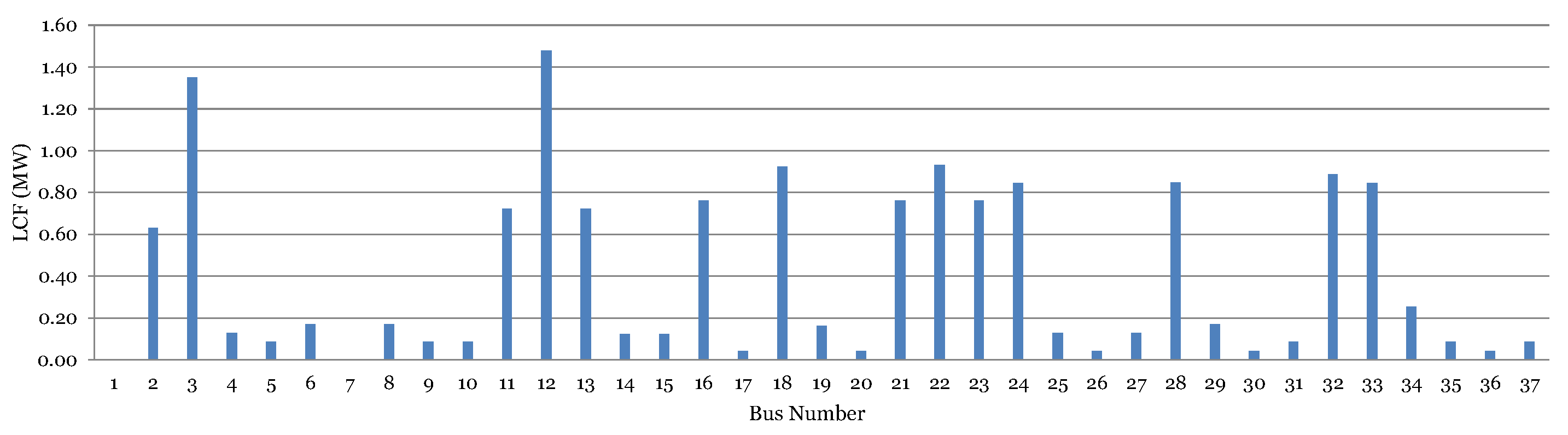
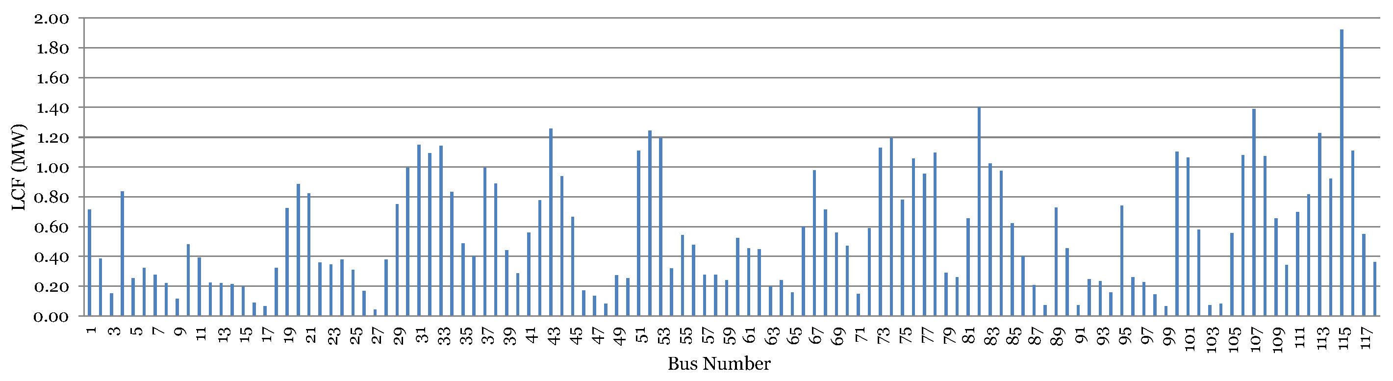
3.3. Load Concentration Factor (LCF)

The LCF of bus “i” in the system is the sum of loads connected to each member bus of set “$C_i$” and the losses across the lines connecting bus “i” to the members of set “$C_i$”. Mathematically,

$$LC{F}_i=\sum _{j\in C_i}{P}_{Dj},$$

(3)

where $P_{Dj}$ is the power demand i.e., load connected at bus “j”. As mentioned above, if there is no load connected to any bus, its $P_{Dj}$ will be taken as zero.

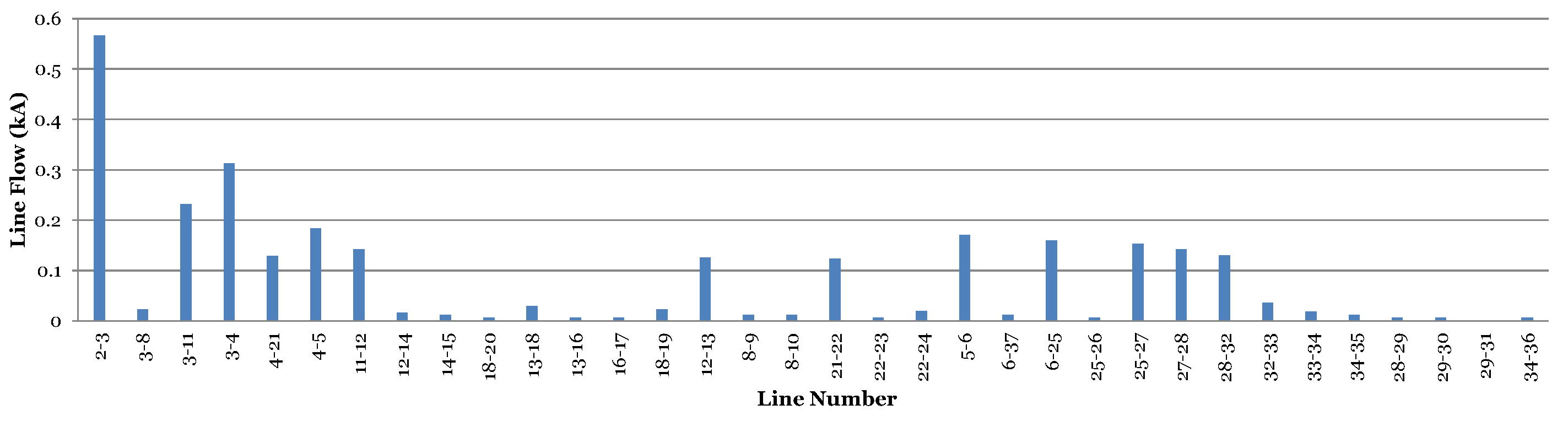
3.4. Selecting the Optimal Locations

It is worth mentioning here that the system may require multiple DGs; hence, there can be different approaches for selecting the optimum location. The most common practice in the research is either finding the optimum locations for the whole system to minimize loss or dividing the whole system into regions and finding an optimum with respect to the specific region. Although the first approach can guarantee the maximum reduction in power loss, it can lead to a non-suitable geographical location. Along with the possibility of improved loss minimization, the later approach can also help to find out the optimum location with respect to availability of geographical space if regions are decided strategically.

3.5. Selection of Optimal Locations in the Systems Under Study

Based on these steps, the $LC{F}_i$ are given in Figure 1 and Figure 2 for IEEE 37 and IEEE 119 node systems, respectively. Ideally, the buses with topmost LCF should have been considered for DG placement, but, due to the high line flows in some lines, the losses on them increase. If the DGs are placed on buses connected to such lines, the losses may increase. The line flows for both networks under study (without DGs) are given in the Figure 3 and Figure 4. Another important consideration was avoiding the DG placement on directly connected buses, which is again to reduce the chances of increased line flows and voltage violations. Therefore, buses (12, 18, 22, 32) and (43, 52, 74, 82, 115) are considered in 37 and 119 node systems, respectively. The case of various regions has not been considered in this work. If it is desired to make regions, the same strategy can be applied for optimal location selection in every region individually.

4. Simultaneous Optimal Sizing

This section elaborates on the mathematical steps taken to formulate expressions for finding optimal DG sizes simultaneously for given specific bus numbers. The generalized method for optimal sizing of “N” DGs simultaneously is explained. To check the accuracy, effectiveness and time for finding an exact solution, the LSF, IA and ELF methods are used. The results are validated by using the slightly modified IEEE 37 and 119 node radial systems with system data given in [37,38]. The node 1 is always considered as a reference and voltage regulated node. The method proposed here not only gives expression for optimal sizing but also a method for finding operational power factors which can ensure the least losses. The extensive mathematical steps taken to finalize the expressions for calculating the size of DGs at “N” buses simultaneously are first introduced followed by steps for finding the operational power factor. The complete set of steps taken to implement these methods is also given.

4.1. Analytical Expressions

For a DG, reactive power injection is given as [27]:

$$Q_{DGi}=a{P}_{DGi},$$

(4)

where

$$\begin{array}{c}a=\left(sign\right)tan\left({cos}^{-1}\left(P{F}_{DG}\right)\right),\end{array}$$

and $sign=+1$ or $-1$ for DG injecting or consuming reactive power. $P{F}_{DG}$ is the power factor of the DG.

Active and reactive power injections at the bus where the DG is installed are given, in terms of active and reactive power demands $P_{D_i}$ and $Q_{D_i}$, as:

$$\begin{array}{c}\hfill P_i=P_{DGi}-P_{Di},\end{array}$$

(5)

$$\begin{array}{c}\hfill Q_i=Q_{DGi}-Q_{Di}=a{P}_{DGi}-Q_{Di}.\end{array}$$

(6)

By substituting Equations (5) and (6) in Equation (1), the active power loss becomes:

$$\begin{array}{c}\hfill P_L=\sum _{i=1}^n\sum _{j=1}^n\left[{\alpha }_{ij}\{(P_{DGi}-P_{Di})P_j+(a{P}_{DGi}-Q_{Di})Q_j)\right\}+{\beta }_{ij}\{(a{P}_{DGi}-Q_{Di})P_j-(P_{DGi}-P_{Di})Q_j\}].\end{array}$$

(7)

It can be proved that the minimum of active power loss of the system can be found if partial derivative of Equation (7) with respect to injected real power from the DG at the ith bus computed equal to zero. Hence, Equation (7) can be written as:

$$\frac{\partial P_L}{\partial P_{DGi}}=2\sum _{j=1}^n[{\alpha }_{ij}(P_j+a{Q}_j)+{\beta }_{ij}(a{P}_j-Q_j)]=0.$$

(8)

As mentioned earlier, the method for calculating the optimum size of “N” DGs is presented here. Suppose that the DGs are to be placed at bus number “$x_1$”,“$x_2$”, ... ,“$x_n$”, where “$x_n$” cannot exceed the total number of buses i.e., “N”, Equation (8) can be re-written as:

$$\frac{\partial P_L}{\partial P_{DG{x}_1}}={\alpha }_{x_1{x}_1}(P_{x_1}+a{Q}_{x_1})+{\beta }_{x_1{x}_1}(a{P}_{x_1}-Q_{x_1})+{\alpha }_{x_1{x}_2}(P_{x_2}+a{Q}_{x_2})+{\beta }_{x_1{x}_2}(a{P}_{x_2}-Q_{x_2})+....+$$

$${\alpha }_{x_1{x}_n}(P_{x_n}+a{Q}_{x_n})+{\beta }_{x_1{x}_n}(a{P}_{x_n}-Q_{x_n})+\sum _{j=1,j\ne 1,2...n}^n({\alpha }_{x_1{x}_j}{P}_j-{\beta }_{x_1{x}_j}{Q}_j)+$$

$$a\sum _{j=1,j\ne 1,2...n}^n({\alpha }_{x_1{x}_j}{Q}_j+{\beta }_{x_1{x}_j}{P}_j)=0$$

$$\frac{\partial P_L}{\partial P_{DG{x}_2}}={\alpha }_{x_2{x}_1}(P_{x_1}+a{Q}_{x_1})+{\beta }_{x_2{x}_1}(a{P}_{x_1}-Q_{x_1})+{\alpha }_{x_2{x}_2}(P_{x_2}+a{Q}_{x_2})+{\beta }_{x_2{x}_2}(a{P}_{x_2}-Q_{x_2})+....+$$

$${\alpha }_{x_2{x}_n}(P_{x_n}+a{Q}_{x_n})+{\beta }_{x_1{x}_n}(a{P}_{x_n}-Q_{x_n})+\sum _{j=1,j\ne 1,2...n}^n({\alpha }_{x_2{x}_j}{P}_j-{\beta }_{x_2{x}_j}{Q}_j)+$$

$$a\sum _{j=1,j\ne 1,2...n}^n({\alpha }_{x_2{x}_j}{Q}_j+{\beta }_{x_2{x}_j}{P}_j)=0$$

$$\begin{array}{c}\hfill ⋮\end{array}$$

$$\frac{\partial P_L}{\partial P_{DG{x}_n}}={\alpha }_{x_n{x}_1}(P_{x_1}+a{Q}_{x_1})+{\beta }_{x_n{x}_1}(a{P}_{x_1}-Q_{x_1})+{\alpha }_{x_n{x}_2}(P_{x_2}+a{Q}_{x_2})+{\beta }_{x_n{x}_2}(a{P}_{x_2}-Q_{x_2})+....+$$

$${\alpha }_{x_n{x}_n}(P_{x_n}+a{Q}_{x_n})+{\beta }_{x_n{x}_n}(a{P}_{x_n}-Q_{x_n})+\sum _{j=1,j\ne 1,2...n}^n({\alpha }_{x_n{x}_j}{P}_j-{\beta }_{x_n{x}_j}{Q}_j)+$$

$$a\sum _{j=1,j\ne 1,2...n}^n({\alpha }_{x_n{x}_j}{Q}_j+{\beta }_{x_n{x}_j}{P}_j)=0.$$

(9)

Let $\left\{\begin{array}{c}{X}_{x_1}={\sum }_{j=1,j\ne x_1,x_2...x_n}^n({\alpha }_{x_1{x}_j}{P}_j-{\beta }_{x_1{x}_j}{Q}_j)+a{\sum }_{j=1,j\ne x_1,x_2...x_n}^n({\alpha }_{x_1{x}_j}{Q}_j+{\beta }_{x_1{x}_j}{P}_j)\\ X_{x_2}={\sum }_{j=1,j\ne x_1,x_2...x_n}^n({\alpha }_{x_2{x}_j}{P}_j-{\beta }_{x_2{x}_j}{Q}_j)+a{\sum }_{j=1,j\ne x_1,x_2...x_n}^n({\alpha }_{x_2{x}_j}{Q}_j+{\beta }_{x_2{x}_j}{P}_j)\\ ⋮\\ X_{x_n}={\sum }_{j=1,j\ne x_1,x_2...x_n}^n({\alpha }_{x_n{x}_j}{P}_j-{\beta }_{x_n{x}_j}{Q}_j)+a{\sum }_{j=1,j\ne x_1,x_2...x_n}^n({\alpha }_{x_n{x}_j}{Q}_j+{\beta }_{x_n{x}_j}{P}_j).\end{array}\right.$

In addition, ${\beta }_{ii}=0$, ${\alpha }_{ij}={\alpha }_{ji}$ and ${\beta }_{ij}=-{\beta }_{ji}$. Thus, by substituting Equations (5) and (6) in set of Equation (9), and arranging for $P_{DG{x}_i}$,

$$\begin{array}{c}\hfill (1+a^2)\sum _{i=1}^n\left(P_{DG{x}_i}{\alpha }_{x_1{x}_i}\right)-\sum _{i=1}^n[P_{D{x}_i}({\alpha }_{x_1{x}_i}+{\beta }_{x_1{x}_i}a)+Q_{D{x}_i}({\alpha }_{x_1{x}_i}a-{\beta }_{x_1{x}_i})]+X_{x_1}=0,\\ \hfill (1+a^2)\sum _{i=1}^n\left(P_{DG{x}_i}{\alpha }_{x_2{x}_i}\right)-\sum _{i=1}^n[P_{D{x}_i}({\alpha }_{x_2{x}_i}+{\beta }_{x_2{x}_i}a)+Q_{D{x}_i}({\alpha }_{x_2{x}_i}a-{\beta }_{x_2{x}_i})]+X_{x_1}=0,\end{array}$$

$$\begin{array}{c}\hfill ⋮\end{array}$$

$$(1+a^2)\sum _{i=1}^n\left(P_{DG{x}_i}{\alpha }_{x_n{x}_i}\right)-\sum _{i=1}^n[P_{D{x}_i}({\alpha }_{x_n{x}_i}+{\beta }_{x_n{x}_i}a)+Q_{D{x}_i}({\alpha }_{x_n{x}_i}a-{\beta }_{x_n{x}_i})]+X_{x_1}=0.$$

(10)

Writing in the form of matrices to solve using Cramer’s rule:

$$AX=B,$$

(11)

where

$$\begin{array}{c}A=(1+a^2)\left[\begin{array}{cccc}{\alpha }_{x_1{x}_1}& {\alpha }_{x_1{x}_2}& \cdots & {\alpha }_{x_1{x}_n}\\ {\alpha }_{x_2{x}_1}& {\alpha }_{x_2{x}_2}& \cdots & {\alpha }_{x_2{x}_n}\\ ⋮& ⋮& \ddots & ⋮\\ {\alpha }_{x_n{x}_1}& {\alpha }_{x_n{x}_2}& \cdots & {\alpha }_{x_n{x}_n}\end{array}\right],X=\left[\begin{array}{c}{P}_{D{G}_1}\\ P_{D{G}_2}\\ ⋮\\ P_{D{G}_n}\end{array}\right],B=\left[\begin{array}{c}{B}_{x_1}\\ B_{x_2}\\ ⋮\\ B_{x_n}\end{array}\right],\end{array}$$

and

$$\begin{array}{c}\hfill B_{x_1}=\sum _{i=1}^n[P_{D{x}_i}({\alpha }_{x_1{x}_i}+{\beta }_{x_1{x}_i}a)+Q_{D{x}_i}({\alpha }_{x_1{x}_i}a-{\beta }_{x_1{x}_i})]-X_{x_1},\\ \hfill B_{x_2}=\sum _{i=1}^n[P_{D{x}_i}({\alpha }_{x_2{x}_i}+{\beta }_{x_2{x}_i}a)+Q_{D{x}_i}({\alpha }_{x_2{x}_i}a-{\beta }_{x_2{x}_i})]-X_{x_2},\end{array}$$

$$\begin{array}{c}\hfill ⋮\end{array}$$

$$B_{x_n}=\sum _{i=1}^n[P_{D{x}_i}({\alpha }_{x_n{x}_i}+{\beta }_{x_n{x}_i}a)+Q_{D{x}_i}({\alpha }_{x_n{x}_i}a-{\beta }_{x_n{x}_i})]-X_{x_n}.$$

(12)

For “N” DGs to be installed, the order of matrices A, B and X is $n\times n$, $n\times 1$ and $n\times 1$, respectively.

It is important to mention that the method finds the optimal active power output desired from DGs to minimize the losses. The reactive power output can be calculated corresponding to the desired power factor using Equation (4). In addition, in this method, the DG sizes depend upon the active and reactive power, whether generation or load, already connected to the system. This means that any equipment or system (storage or generation, etc.) that can be represented in the form of active and reactive power can be used by taking care of respective sign notation i.e., positive for generations and negative for loads. In this way, the method can be used to include any type of existing generations as has been done in [35].

4.2. Operational Power Factor

To make these expressions useable for practical cases, the power factor demanded from a DG is also incorporated. In improved analytical (IA) method, combined load power factor (CLPF) is considered as the optimal power factor. This approach of finding the optimal power factor has produced good results, but the CLPF cannot be useful for the systems with higher reactive power demand such as IEEE 119 node radial system considered in this work. CLPF for this system was about 0.79, which is not preferred in most of the distribution grid codes.

For a generator, power factor near unity is preferred but, sometimes, it is not possible in practical systems to keep power factor near unity. Therefore, a range of considered power factor in this work is taken to be 0.90–1.00. On this ground, the suggested power factor is named as the operational power factor. As already mentioned, the proposed method is considerably fast with respect to the other contemporary methods, an exhaustive approach for finding the operational power factor is suggested in this work. Starting from power factor of 0.90, the method found optimal DG sizes and losses with a step size of 0.01 until either a unity power factor is reached or active power loss starts increasing then those for power factor of previous step. This helped in finding operational power factor without significant increase in the total simulation time. Although the primary objective was active power loss minimization, the voltage profile is also improved significantly in comparison to the other stated methods.

Although the method stops operating after it finds that the losses are increased for a power factor as compared to the previous step, the results of the complete range are presented in Section 6.2. The operational power factor for the 37 node and 119 node radial systems is 0.97 and 0.90, respectively.

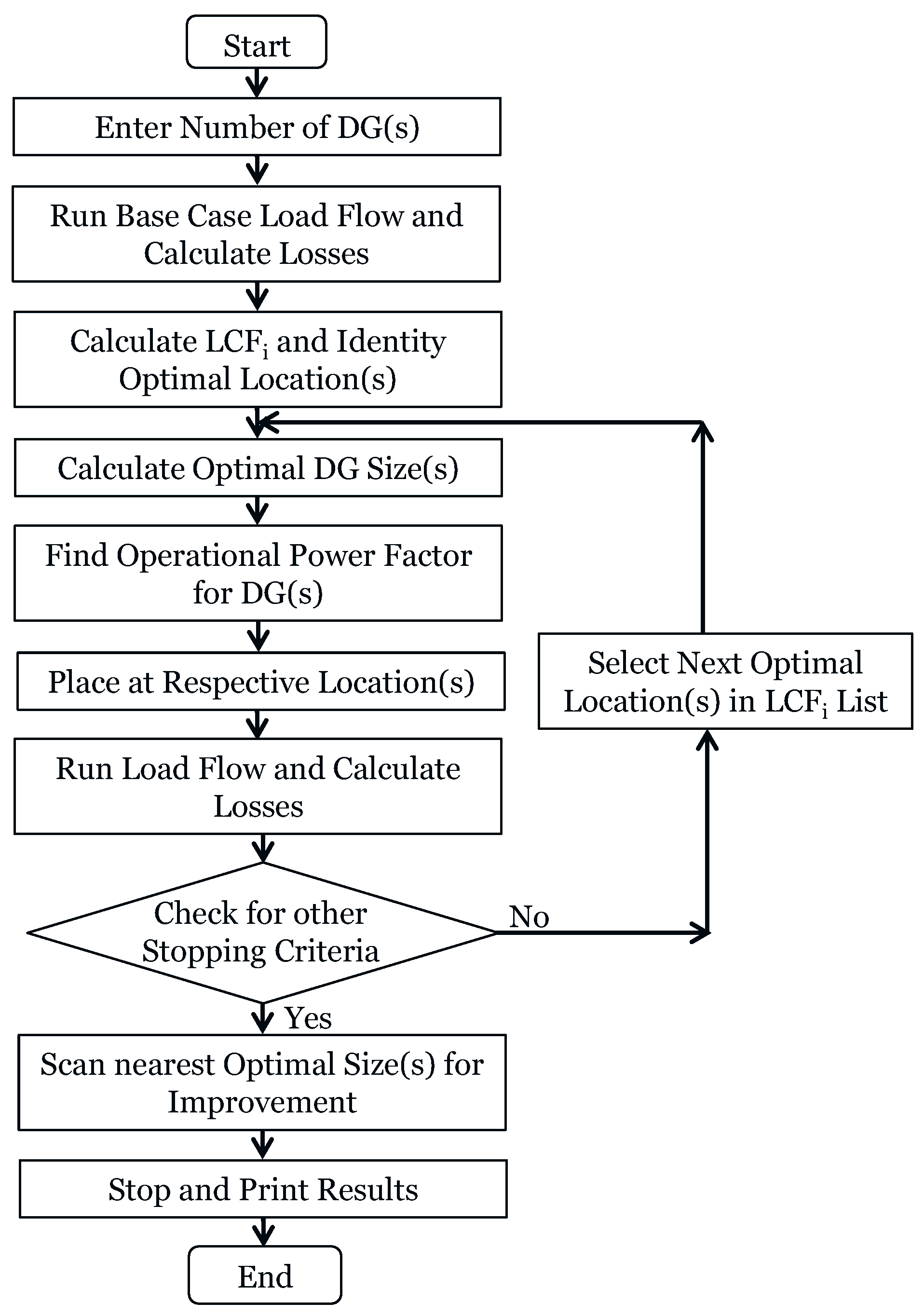
4.3. Algorithm for Optimal Sizes Calculation

Figure 5 illustrates the flow chart of the computational steps needed to find the results based on proposed analytical expressions. The power of the slack bus is kept positive in order to limit the chances of increasing the losses.

• Enter the base case network.
• Enter the desired number of DGs to be placed.
• Run base case load flow and calculate losses using Equation (1).
• For all the buses in a region, calculate the $LC{F}_i$ and arrange the buses in descending order with respect to this.
• Choose “N” buses for placing “N” DGs. The initial set of bus numbers will contain the bus(es) with highest LCF in each region.
• Based on input data in step (4), find the optimal size of DGs using the expression given in Equation (11).
• Calculate operational power factor of DG using exhaustive method.
• Stop if:

  • The sum of power of DGs to be installed is less than the total power demand plus losses.
  • The bus voltages are within a permissible limit.
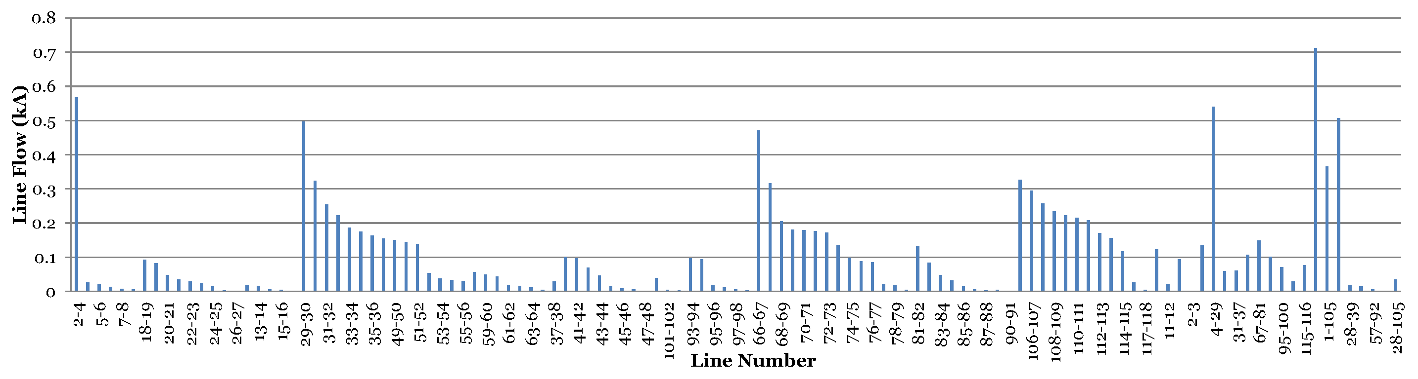
  • The lines are not overloaded.
  Else, look for new locations by using these steps.

  • Try to change only one bus in the region from the set of bus numbers chosen in step (4) i.e., for placing n DGs, $(n-1)$ buses will remain the same.
  • The most suitable candidate for the changed bus will be the one which has the least difference in LCF from the LCF of a previously selected bus, while staying in the same region.
  • In case of a clash between any two or more regions for the selection of the second highest LCF bus, priority will be given to the bus which carries the highest load.
  Go to step (6)
• Place sized DGs in the system and calculate losses using Equation (1).
• To check for better sizes, optimal sizes in nearest proximity can also be checked.
• To check for even better solutions, the next candidate buses in the list of LCF can also be checked, but experiments showed that this leads to zero or negligible improvements.

5. Comparative Studies

For the purpose of comparison and validation, the following methods have been implemented.

5.1. Loss Sensitivity Factor

The LSF method [26] for selection of optimum location is based on the principle of linearization of the original exact loss curve around an initial operating point. In this way, the size of the solution space is reduced. Based on Equation (1), the LSF of the ith bus is given as:

$${\mathrm{L}SF}_i=\partial P_L/\partial P_i=2\sum _{j=1}^n({\alpha }_{ij}{P}_j-{\beta }_{ij}{Q}_j).$$

(13)

The LSFs for all buses in the systems are calculated to arrange them in descending order. The top 20% of buses in the LSF list are selected for iterative placement and sizing of the DGs. For each iteration, the losses are calculated by placing the DGs from zero up to the maximum, which is changed in small steps. The size with least losses is selected. For placing the next DG, LSFs are calculated again and the DG is placed using the very same method.

5.2. Improved Analytical Method

The improved analytical (IA) method, proposed in [28], calculates the optimum sizes of multiple DGs iteratively. This advanced technique is presented in the latest literature and is used here for comparison and validation. The iterations for finding the optimum locations have been removed and only the optimum DG sizes are calculated for respective buses to reduce the computation time.

5.3. Exhaustive Load Flow Method

This method is considered to be the most suitable and accurate method in literature for optimizing the location and sizing of DGs. It is presented in [39]. This method places one DG at a time on a bus, and increases its output power from zero to some specified maximum value in steps. For every iterative step, it finds the active power losses. At the end of this scanning of every bus, it stores the size of the DG corresponding to the least losses. The same practice continues until the specified stopping criteria is reached, which is usually either the sum of all DG outputs to be equal or greater than total demand in the network or the maximum number of DGs.

6. Results

6.1. Experiments/Use Cases

Two different systems, IEEE 37 and 119 nodes, given in Figure 6 and Figure 7, have been considered for testing the proposed methodology. Details of total active power demands and losses without DG are summarized in

Table 1. Base case system data.

Parameters	37 Node System	119 Node System
Active Power Demand	4.98 MW	22.71 MW
Reactive Power Demand	1.35 MVar	17.04 MVar
Active Power Loss without DGs	281.77 kW	1440.89 kW
Min Voltage in Network	0.878 p.u	0.869 p.u
Max Voltage in Network	1.000 p.u	1.000 p.u

. Our software is developed in Python coupled with DIgSILENT PowerFactory (DSPF) through Application Programming Interface (API).

The DSPF is a widely used commercial tool for studying the power systems. Its functionality is expanded further by coupling it with Python, which helped to program the complex equations very easily. Further details about this can be found in [40]. Another possibility of coupling DSPF with MATLAB is given in [41]. The software is mainly operated from a Python command line environment, which computes the base case losses, finds optimum locations for DG placement based on LCF, then computes the optimum sizes of multiple DGs. Finally, the losses are calculated after placing these DGs. The Newton–Raphson method was used to solve power flow of the systems. A standard PC with Intel Xeon Processor W3505 and 12 GB RAM is used for simulation. To generalize, the DGs with the ability of injecting both active and reactive power are considered. The operational power factor and power factor of 0.95 are used for calculating the DG sizes at static demand. In addition, the upper and lower bus voltage limits are kept between ±6% of nominal i.e., 1.06 and 0.94 p.u. [42]. Based on the network data used, the $I_{max}$ is taken to be 0.8 kA. The size of the DG can vary between some kilowatts to 300 MW [43] but depends upon the capacity of the power system and can be considered maximum up to the total power demand plus the losses [9].

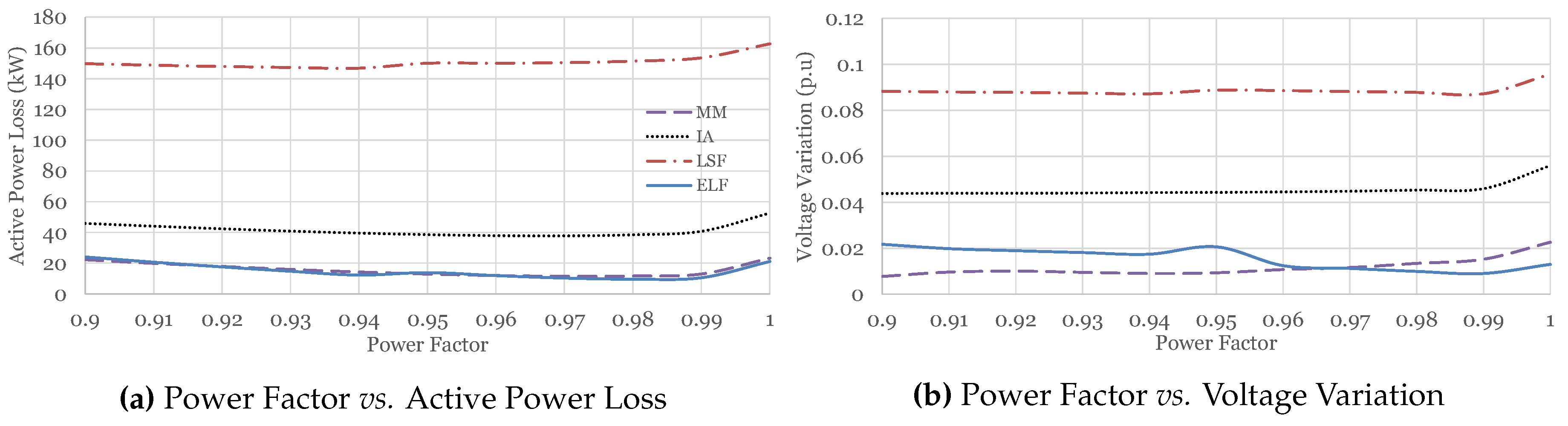
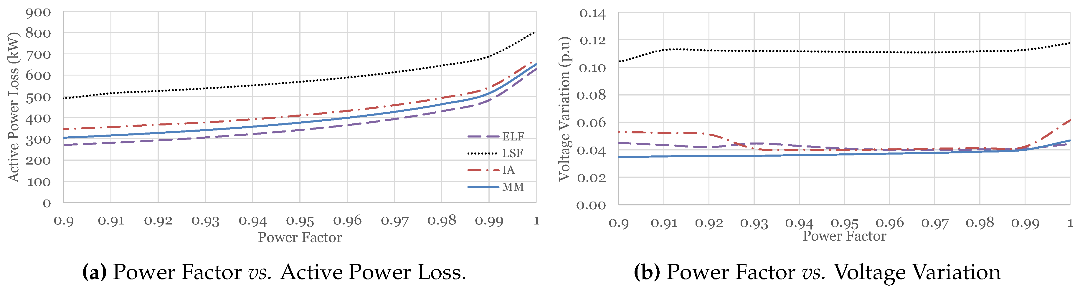
6.2. Operational Power Factor Test Results

The DGs considered throughout this work are capable of injecting both real and reactive power. Hence, the impact of the power factor is also important. For results shown in Figure 8a and Figure 9a, it can be clearly seen that the operation beyond the operational power factor increases the losses, with either of the methods discussed here. The LSF method appeared to be the least efficient method, whereas the ELF and Mohsin method (MM) methods produced nearly the same as well as the best results. The IA method also produced good results in comparison to the LSF but was outperformed by the ELF and MM methods. Similar trends of loss reduction is observed for both test systems studied in this work.

Another important result that can be drawn from the graphs given in Figure 8b and Figure 9b is about the voltage stability of the system at operational power factor. Not only is the voltage profile improved (as given in Section 6.4), but the voltage variation is also reduced. Voltage variation is given as the difference between the maximum and minimum voltage appearing in the network (at any bus) for a specific power factor. For the MM method, the voltage variation is the minimum over most of the considered range of power factors, which clearly highlights the usefulness of the presented method.

Based on the results of this section, it is proven that the power factor selection is also an important point which must be properly addressed while optimizing the size and location for placement of DGs.

6.3. Active Power Loss Minimization Results

The sizes of the DGs were calculated for the given number of DGs. It is never considered to be the only possibility of, for example, four DGs in the case of IEEE 37 node system. Moreover, the sizes of DGs found here are to ensure the least possible losses, and, subsequently, the voltage profile improvement. After DG installation, in operational phase, increasing or decreasing the sizes beyond the calculated sizes is possible. Consequently, non-optimal sizes will be resulted; hence, the losses will vary.

In this case study, it was considered that the total power supplied by DG is not more than total demand [28]. This is done because supplying power to the external grid may increase the losses due to increased line flows. As in real networks, the reverse power flow can happen, and this constraint can be altered to allow a certain amount of power to be delivered to the external grid. The sizes of DGs and losses will be different.

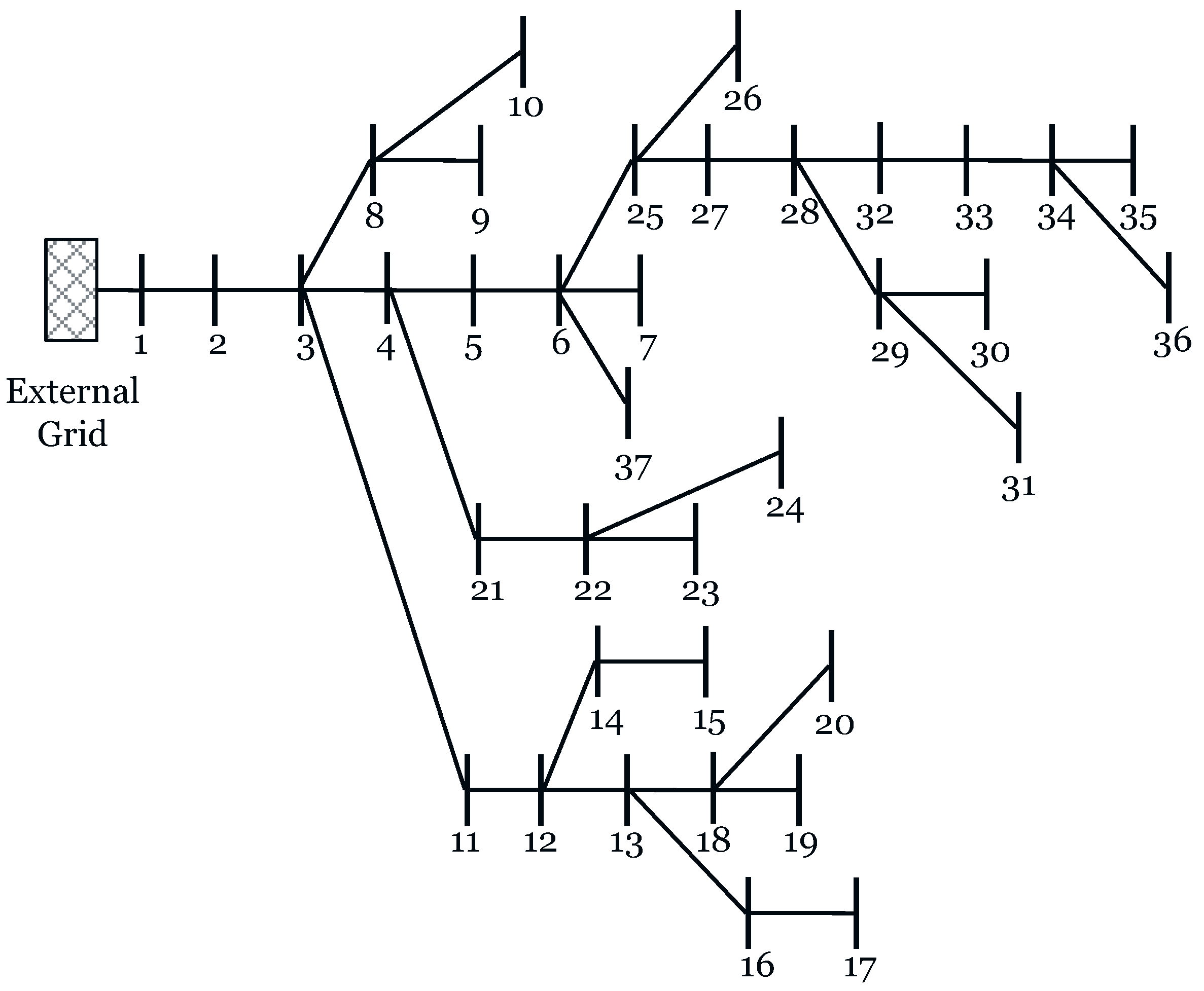
6.3.1. 37 Bus System

The simulation results with the proposed methodology and other mentioned techniques have been summarized in

Table 2. DG placement by different methods for IEEE 37 node system at operational power factor.

Case	Method	Installed DG Schedule (MW)					DG (MW)	Ploss (kW)	Loss Red (%)	Time (s)
No DG	Total Real Load = 4.977 MW						-	281.77	-	-
4 DGs	LSF	Bus	25	2	7	37	7.5	150.465	46.60	35.34
		Size	2.5	5	0	0
	IA	Bus	5	19	24	33	3.23	37.798	86.52	18.32
		Size	0.67	1.05	0.51	1
	ELF	Bus	11	13	22	32	4.5	10.318	96.33	117.44
		Size	0.5	1.5	1	1.5
	MM	Bus	12	18	22	32	3.5	11.479	95.92	12.54
		Size	0.6	0.6	0.9	1.4

for the IEEE 37 node system. The losses for no DG case and after placement of optimally sized DGs with various techniques along with computation time are shown in Table 2.

From these results, the proposed method proves its superiority both in terms of simulation time and loss reduction. The IA method appears to be the nearest in terms of both of these objectives while the LSF method is not only slow in finding the optimum size but also gives poor loss reduction. For the 37 node system, loss reductions of 46.60%, 86.52%, 96.33% and 95.92% is observed for LSF, the IA method, the ELF method and our proposed method (MM), respectively. It is worth mentioning that the ELF method produced slightly better results in comparison to the method presented in this work because it scans all the buses iteratively for every possible size.

Optimal placement of DG is a planning phase issue where the computational time of a few minutes may not be very important but is presented here for the sake of comparison among different methods. Comparing the computational time for placement of four DGs with different techniques discussed here shows the advantage of our proposed methodology. The nearest competitor in terms of simulation time taken is the IA method, which took about 33% more time than the proposed method. Similarly, the LSF method, being iterative over the limited number of buses, took a considerably high amount of time (about more than five times higher) for placing four DGs. Despite being slightly better at reducing the losses, the ELF method is highly demanding, as can be seen from the simulation time taken by it. The time taken by the ELF method to reach the final solution is approximately 33 times more than that of the MM method. It is important to note that the ELF method could be made faster by making the step size of DG size bigger, which would have ultimately adversely affected the optimal sizes and hence the loss reduction. Hence, the proposed method appears to be the best in respect to both the loss reduction and computational time.

External infeed for this system was reported to be 5.40 MVA in the base case, which was reduced to 1.46 MVA after optimal placement of DGs.

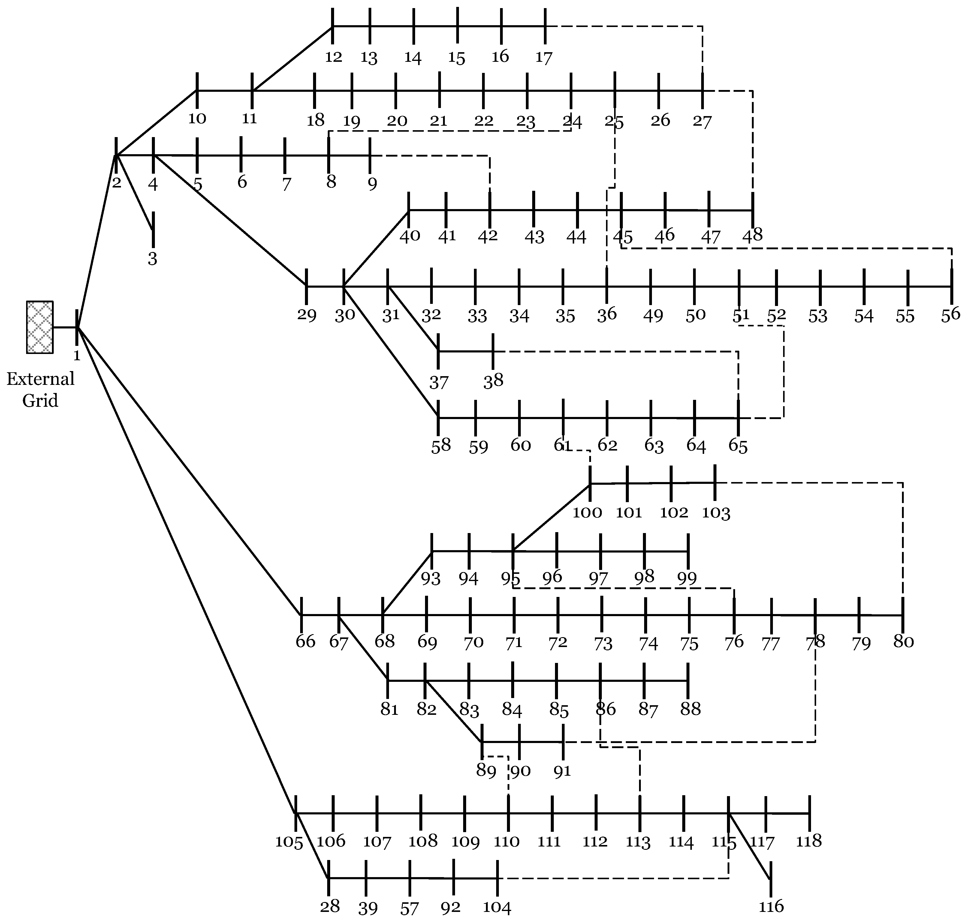
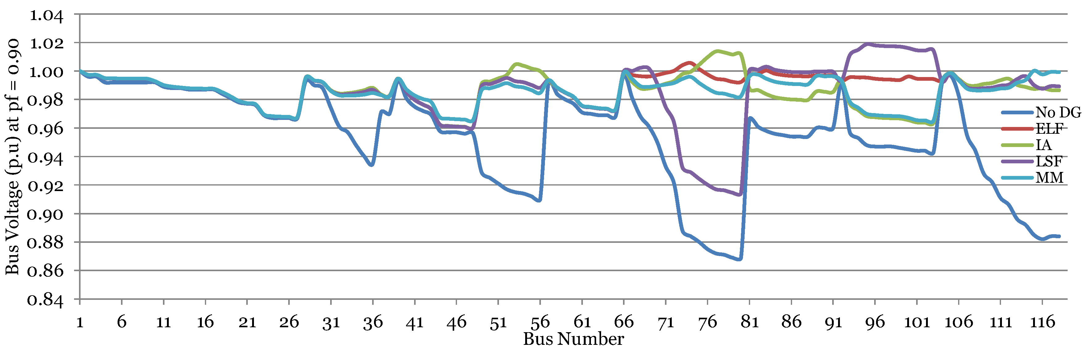
6.3.2. 119 Bus System

Table 3. DG placement by different methods for IEEE 119 node system at operational power factor.

Case	Method	Installed DG Schedule (MW)						DG (MW)	Ploss (kW)	Loss Red (%)	Time (s)
No DG	Total Real Load = 22.71 MW							-	1440.89	-	-
5 DGs	LSF	Bus	52	69	83	95	114	15.5	490.73	65.94	619.01
		Size	3.5	3	2.5	3	3.5
	IA	Bus	53	77	82	112	116	12.1	345.24	76.04	106.59
		Size	3.6	3.1	1.7	2.4	1.3
	ELF	Bus	52	74	83	100	114	14	270.9	81.20	3077.71
		Size	3.5	3	2.5	1.5	3.5
	MM	Bus	43	52	74	82	115	12.8	305.2	78.82	42.95
		Size	0.4	3.3	2.9	2.8	3.4

presents the simulation results for the IEEE 119 node system in the same fashion as they were done for the 37 node system. It can be seen that the proposed methodology could find the optimum sizes for reduction of losses in the system considerably faster. In addition, the sizes found depict the effectiveness of the proposed analytic expression for simultaneous sizing of DGs because the loss reduction is higher among all the presented techniques except the ELF method. The LSF method is proved to be the least efficient in terms of simulation time and optimum sizes that can reduce losses to the lowest level. Loss reduction with the LSF method, the IA method, the ELF method and the proposed method are 65.94%, 76.04%, 81.20% and 78.82%, respectively. The ELF method is proved better in loss reduction but at the cost of very high computation time.

The proposed methodology can find the optimum size for five DGs in the 119 node system approximately 2.5 times faster than by the IA method. The LSF method, being an iterative technique for finding the optimum size, consumes 14.4 times more time as compared to the proposed method. Although slightly better in loss reduction, the ELF method consumed approximately 72 times more time than the proposed method. Based on these important observations, the proposed method outperformed the other methods given here.

As per most of the grid code requirements and preferences, the most desired power factor is 0.95. The results of which are summarized in the

Table 4. DG placement by different methods for IEEE 119 node system at 0.95 power factor.

Case	Method	Installed DG Schedule (MW)						DG (MW)	Ploss (kW)	Loss Red (%)	Time (s)
No DG	Total Real Load = 22.71 MW							-	1440.89	-	-
5 DGs	LSF	Bus	46	52	82	95	114	14	568.48	60.55	649.12
		Size	1	3.5	3	3	3.5
	IA	Bus	53	74	82	112	117	12.3	409.9	71.55	109.67
		Size	3.7	2.7	1.8	2.4	1.7
	ELF	Bus	52	75	83	100	114	14	341.28	76.31	3107.33
		Size	3.5	3	2.5	1.5	3.5
	MM	Bus	43	52	74	82	115	13	375.96	73.91	44.28
		Size	0.4	3.3	3	2.8	3.5

. These results show the same trends in loss reduction and simulation time as were given in Table 3. Slightly higher losses are observed because of the fact that this is not an optimal power factor for this system. This also speaks about the need for optimizing the power factor.

In this system, external infeed of 30.16 MVA in the base case and 15.05 MVA after optimal placement of DGs was recorded.

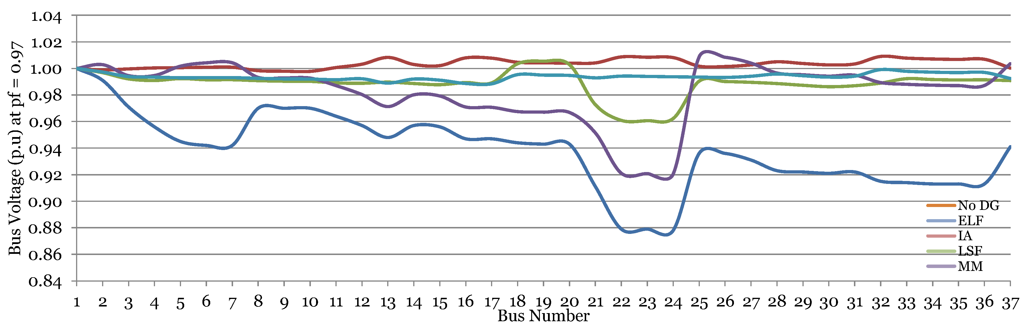
6.4. Voltage Profile Improvement Results

An additional advantage of the optimal sitting and sizing of DGs with the proposed method is depicted clearly in Figure 10 and Figure 11. These graphs were taken when the system was operating at the operational power factor proposed in Section 4.2. As mentioned in the Table 1 and can also be seen in these figures, the minimum voltage in either network is about 0.87 p.u. approximately, whereas the maximum voltage is 1.000 p.u., which appeared at the node where the external grid is connected and is a voltage regulated node. After DG placement, all the methods improved the voltage in the network; however, the voltage improvement is varying. It is already shown in Figure 8b and Figure 9b that voltage variation (the difference between maximum and minimum voltages appearing in the network) is the lowest with the method proposed here.

For the 37 node network, the minimum voltage observed after optimal DG placement was 0.998 p.u. with the ELF method, whereas with the proposed method (MM), the voltage was 0.988 p.u. Moreover, the highest voltage observed with ELF method of optimal DG placement was 1.009 p.u., and, with the proposed method, it was 1.000 p.u. The IA method also brought the minimum voltage to the permissible limit of 0.961 p.u. and maximum voltage to 1.005 p.u. Although the voltage improvement by IA method is within the allowed band, it is closer to the minimum level, which makes it prone to falling below with small variation in loads or generations. The LSF method was unable to increase the minimum voltage to the permissible level.

From Figure 11, it is clear that the proposed method outperformed the other methods where the minimum voltage was 0.965 p.u. and maximum voltage was 1.000 p.u. The ELF and IA methods also improved minimum voltage to 0.961 p.u. each, but the maximum voltage was 1.006 p.u. and 1.014 p.u., respectively. For the LSF method, minimum voltage was again out of the permissible bounds and appeared to be 0.915 p.u., whereas the maximum voltage was 1.019 p.u.

As a final comment, it is said that, for a network, it is not only required to keep maximum and minimum voltages within the limits, but the difference between these two should also be kept closer to zero to make the system more stable with respect to the voltage.

7. Conclusions

This paper explains a novel method for finding the optimal bus numbers for placing multiple DGs. The method is based on load concentration faced directly by the bus or through directly connected buses. Based on the optimal locations selected, analytical expressions for the optimal sizes of single or multiple DGs are derived for a large scale distribution system. The generalized steps to derive the analytic expressions for simultaneous optimum sizing, which also include the impact of all DGs on each other, are presented.

The exhaustive method for selecting operational power factor required from a DG is also incorporated, resulting in the versatility of the derived expressions to be used for DGs with both active and reactive power generation capabilities. Moreover, the LSF, IA and ELF methods have been presented. The proposed methodology for simultaneous optimal sizing of multiple DGs is confirmed to be effective and efficient in comparison with LSF and IA both in terms of minimizing the losses and simulation time. For the ELF method, the results of the presented methods are comparable in terms of loss minimization but superior for voltage profile improvement and simulation time.

The proposed methodology is the general set of steps that can be applied for any number of DGs. In this work, the cases of only four DGs in an IEEE 37 node and five DGs in an IEEE 119 bus systems are discussed. Another important conclusion is the need for optimizing the power factor that a DG must provide within the limit of grid code requirements. It is observed that the DGs with optimal power factor can reduce the losses further if kept within the limits. Hence, to achieve the maximum benefits from DG(s), their location, size and power factor must be properly chosen.

The study presents a novel, useful and highly competitive method for planning and decision support before implementing and connecting DGs to the electric power grid. It makes unused and normally wasted optimization potential accessible and reduces losses and transmission and distribution system stress.

References

1. Singh, D.; Singh, D.; Verma, K. GA based energy loss minimization approach for optimal sizing & placement of distributed generation. Int. J. Knowl. Based Intell. Eng. Syst. 2008, 12, 147–156. [Google Scholar]
2. Georgilakis, P.; Hatziargyriou, N. Optimal distributed generation placement in power distribution networks: Models, methods, and future research. IEEE Trans. Power Syst. 2013, 28, 3420–3428. [Google Scholar] [CrossRef]
3. Taylor, M.; Daniel, K.; Ilas, A.; So, E. Renewable Power Generation Costs in 2014; International Renewable Energy Agency: Masdar City, Abu Dhabi, UAE, 2015. [Google Scholar]
4. Li, W.; Joos, G.; Belanger, J. Real-time simulation of a wind turbine generator coupled with a battery supercapacitor energy storage system. IEEE Trans. Ind. Electron. 2010, 57, 1137–1145. [Google Scholar] [CrossRef]
5. Pigazo, A.; Liserre, M.; Mastromauro, R.; Moreno, V.; Dell’Aquila, A. Wavelet-based islanding detection in grid-connected PV systems. IEEE Trans. Ind. Electron. 2009, 56, 4445–4455. [Google Scholar] [CrossRef]
6. Yao, W.; Chen, M.; Matas, J.; Guerrero, J.; Ming Qian, Z. Design and analysis of the droop control method for parallel inverters considering the impact of the complex impedance on the power sharing. IEEE Trans. Ind. Electron. 2011, 58, 576–588. [Google Scholar] [CrossRef]
7. Guerrero, J.M.; Vasquez, J.C.; Matas, J.; de Vicuna, L.G.; Castilla, M. Hierarchical control of droop-controlled AC and DC microgrids—A general approach toward standardization. IEEE Trans. Ind. Electron. 2010, 58, 158–172. [Google Scholar] [CrossRef]
8. Guerrero, J.; Matas, J.; de Vicuna, L.G.; Castilla, M.; Miret, J. Decentralized control for parallel operation of distributed generation inverters using resistive output impedance. IEEE Trans. Ind. Electron. 2007, 54, 994–1004. [Google Scholar] [CrossRef]
9. Hung, D.Q.; Mithulananthan, N.; Bansal, R. Analytical strategies for renewable distributed generation integration considering energy loss minimization. Appl. Energy 2013, 105, 75–85. [Google Scholar] [CrossRef]
10. Atwa, Y.; El-Saadany, E.; Salama, M.; Seethapathy, R. Optimal renewable resources mix for distribution system energy loss minimization. IEEE Trans. Power Syst. 2010, 25, 360–370. [Google Scholar] [CrossRef]
11. Antonova, G.; Nardi, M.; Scott, A.; Pesin, M. Distributed generation and its impact on power grids and microgrids protection. In Proceedings of the 2012 65th Annual Conference for Protective Relay Engineers, College Station, TX, USA, 2–5 April 2012; pp. 152–161.
12. Standard EN 50160. Voltage Characteristics of Public Distribution Systems; CENELEC: Brussels, Belgium, 2010. [Google Scholar]
13. Liu, Y.; Bebic, J.; Kroposki, B.; De Bedout, J.; Ren, W. Distribution system voltage performance analysis for high-penetration PV. In Proceedings of the IEEE Energy 2030 Conference, ENERGY 2008, Atlanta, GA, USA, 17–18 November 2008; pp. 1–8.
14. Moradi, M.; Abedini, M. A combination of genetic algorithm and particle swarm optimization for optimal {DG} location and sizing in distribution systems. Int. J. Electr. Power Energy Syst. 2012, 34, 66–74. [Google Scholar] [CrossRef]
15. Mithulananthan, N.; Oo, T.; Phu, L.V. Distributed generator placement in power distribution system using genetic algorithm to reduce losses. Thammasat Int. J. Sci. Technol. 2004, 9, 55–62. [Google Scholar]
16. Singh, D.; Singh, D.; Verma, K. GA based optimal sizing & placement of distributed generation for loss minimization. Int. J. Intell. Technol. 2007, 2, 263–269. [Google Scholar]
17. De Souza, B.; de Albuquerque, J. Optimal placement of distributed generators networks using evolutionary programming. In Proceedings of the Transmission Distribution Conference and Exposition: Latin America, Caracas, Venezuela, 15–18 August 2006; pp. 1–6.
18. El-Zonkoly, A. Optimal placement of multi-distributed generation units including different load models using particle swarm optimisation. IET Gen. Transm. Distrib. 2011, 5, 760–771. [Google Scholar] [CrossRef]
19. Bouhouras, A.S.; Sgouras, K.I.; Gkaidatzis, P.A.; Labridis, D.P. Optimal active and reactive nodal power requirements towards loss minimization under reverse power flow constraint defining DG type. Int. J. Electr. Power Energy Syst. 2016, 78, 445–454. [Google Scholar] [CrossRef]
20. Wang, C.; Nehrir, M. Analytical approaches for optimal placement of distributed generation sources in power systems. IEEE Trans. Power Syst. 2004, 19, 2068–2076. [Google Scholar] [CrossRef]
21. Ziari, I.; Ledwich, G.; Ghosh, A.; Cornforth, D.; Wishart, M. Optimal allocation and sizing of DGs in distribution networks. In Proceedings of the 2010 IEEE Power and Energy Society General Meeting, Minneapolis, MN, USA, 25–29 July 2010; pp. 1–8.
22. Lee, S.H.; Park, J.W. Selection of optimal location and size of multiple distributed generations by using Kalman filter algorithm. IEEE Trans. Power Syst. 2009, 24, 1393–1400. [Google Scholar]
23. Khatod, D.; Pant, V.; Sharma, J. Evolutionary programming based optimal placement of renewable distributed generators. IEEE Trans. Power Syst. 2013, 28, 683–695. [Google Scholar] [CrossRef]
24. Liu, Z.; Wen, F.; Ledwich, G. Optimal siting and sizing of distributed generators in distribution systems considering uncertainties. IEEE Trans. Power Deliv. 2011, 26, 2541–2551. [Google Scholar] [CrossRef]
25. Kayal, P.; Kar, S.; Upadhyaya, A.; Chanda, C. Optimal sizing of multiple distributed generation units connected with distribution system using PSO technique. In Proceedings of the 2012 International Conference on Emerging Trends in Electrical Engineering and Energy Management, Chennai, India, 13–15 December 2012; pp. 229–234.
26. Acharya, N.; Mahat, P.; Mithulananthan, N. An analytical approach for DG allocation in primary distribution network. Int. J. Electr. Power Energy Syst. 2006, 28, 669–678. [Google Scholar] [CrossRef]
27. Hung, D.Q.; Mithulananthan, N.; Bansal, R. Analytical expressions for DG allocation in primary distribution networks. IEEE Trans. Energy Convers. 2010, 25, 814–820. [Google Scholar] [CrossRef]
28. Hung, D.Q.; Mithulananthan, N. Multiple distributed generator placement in primary distribution networks for loss reduction. IEEE Trans. Ind. Electr. 2013, 60, 1700–1708. [Google Scholar] [CrossRef]
29. Kamel, R.; Kermanshahi, B. Optimal size and location of distributed generations for minimizing power losses in a primary distribution network. Sci. Iran. Trans. D Comput. Sci. Eng. Electr. Eng. 2009, 16, 137–144. [Google Scholar]
30. Viral, R.; Khatod, D. An analytical approach for sizing and siting of DGs in balanced radial distribution networks for loss minimization. Int. J. Electr. Power Energy Syst. 2015, 67, 191–201. [Google Scholar] [CrossRef]
31. Carpinelli, G.; Celli, G.; Pilo, F.; Russo, A. Embedded generation planning under uncertainty including power quality issues. Eur. Trans. Electr. Power 2003, 13, 381–389. [Google Scholar] [CrossRef]
32. Haesen, E.; Driesen, J.; Belmans, R. Robust planning methodology for integration of stochastic generators in distribution grids. IET Renew. Power Gen. 2007, 1, 25–32. [Google Scholar] [CrossRef]
33. Evangelopoulos, V.; Georgilakis, P. Optimal distributed generation placement under uncertainties based on point estimate method embedded genetic algorithm. IET Gen. Transm. Distrib. 2014, 8, 389–400. [Google Scholar] [CrossRef]
34. Singh, A.; Parida, S. Selection of load buses for DG placement based on loss reduction and voltage improvement sensitivity. In Proceedings of the 2011 International Conference on Power Engineering, Energy and Electrical Drives (POWERENG), Malaga, Spain, 11–13 May 2011; pp. 1–6.
35. Shahzad, M.; Ullah, I.; Palensky, P.; Gawlik, W. Analytical approach for simultaneous optimal sizing and placement of multiple Distributed Generators in primary distribution networks. In Proceedings of the 2014 IEEE 23rd International Symposium on Industrial Electronics (ISIE), Istanbul, Turkey, 1–4 June 2014; pp. 2554–2559.
36. Kothari, D.; Dhillon, J. Power System Optimization; Prentice-Hall: New Dehli, India, 2004. [Google Scholar]
37. IEEE PES Distribution System Analysis Subcommittee’s Distribution Test Feeder Working Group. Available online: http://ewh.ieee.org/soc/pes/dsacom/testfeeders/ (accessed on 11 April 2016).
38. Zhang, D.; Fu, Z.; Zhang, L. An improved TS algorithm for loss-minimum reconfiguration in large-scale distribution systems. Electr. Power Syst. Res. 2007, 77, 685–694. [Google Scholar] [CrossRef]
39. Hung, D.Q.; Mithulananthan, N. DG allocation in primary distribution systems considering loss reduction. In Handbook of Renewable Energy Technology; Chapter 23; World Scientific: Singapore, 2011; pp. 587–635. [Google Scholar]
40. Ahmad, I.; Kazmi, J.H.; Shahzad, M.; Palensky, P. Co-simulation framework based on power system, AI and communication tools for evaluating smart grid applications. In Proceedings of the IEEE PES Innovative Smart Grid Technologies 2015 Asian Conference, Bangkok, Thailand, 3–6 November 2015.
41. Latif, A.; Shahzad, M.; Palensky, P.; Gawlik, W. An alternate PowerFactory Matlab coupling approach. In Proceedings of the 2015 International Symposium on Smart Electric Distribution Systems and Technologies (EDST), Vienna, Austria, 8–11 September 2015; pp. 486–491.
42. Siano, P.; Ochoa, L.; Harrison, G.; Piccolo, A. Assessing the strategic benefits of distributed generation ownership for DNOs. IET Gen. Transm. Distrib. 2009, 3, 225–236. [Google Scholar] [CrossRef]
43. Ackermann, T.; Andersson, G.; Söder, L. Distributed generation: A definition. Electr. Power Syst. Res. 2001, 57, 195–204. [Google Scholar] [CrossRef]
Figure 1. Load concentration factors for 37 node system.
Energies 09 00287 g001
Figure 2. Load concentration factor for 119 node system.
Energies 09 00287 g002
Figure 3. Line flows for 37 node system.
Energies 09 00287 g003
Figure 4. Line flows for 119 node system.
Energies 09 00287 g004
Figure 5. Flowchart of optimal placement.
Energies 09 00287 g005
Figure 6. IEEE 37 node network.
Energies 09 00287 g006
Figure 7. IEEE 119 node network.
Energies 09 00287 g007
Figure 8. Operational power factor for 37 node system.
Energies 09 00287 g008
Figure 9. Operational power factor for 119 node system.
Energies 09 00287 g009
Figure 10. Voltage profile for 37 node system with different methods (pf = 0.97).
Energies 09 00287 g010
Figure 11. Voltage profile for 119 node system with different methods (pf = 0.90).
Energies 09 00287 g011