Short-Circuit Calculation in Distribution Networks with Distributed Induction Generators

Abstract

This paper presents an improved current source equivalent model method to determine the short-circuit current of a distribution system with multiple fixed-speed and variable-speed induction generators (IGs). The correlation coefficients of flux components between stator and rotor under the unsymmetrical fault are analyzed using the positive and negative sequence steady-state equivalent circuits of an IG. The terminal voltage and current responses of fixed-speed and variable-speed IGs with and without the rotor slip changes under different penetration levels are compared to investigate the coupling relation between the short-circuit currents of IGs and the nodal voltages in the distribution network. Then the transient equivalent potential of an IG at the grid fault instant is derived. Sequence components of the short-circuit current in the network can be determined using the proposed technique. The correctness of the proposed method is verified using dynamic simulation.

1. Introduction

The increased penetration of renewable power has resulted in more distributed generators (DGs) embedded in distribution networks. The integration of large-scale DGs into the distribution network changes the distribution of power flow and short-circuit currents, and leads the short-circuit current contribution of the DGs to affect the power system protection and reclosing [1]. DGs include synchronous generators, induction generators (IGs), and other power sources with electronic interfaces; of these types, the squirrel-cage IG has received increased attention in distribution networks because of its low cost, small size, and low maintenance requirements [2]. When short-circuit faults occur, IGs are unable to maintain their terminal voltage without an external excitation current, because they have different short-circuit current characteristics compared with synchronous generators [3]. IG technology is based on the relatively mature induction motor (IM), and the difference is that the IG tends to excessively accelerate instead of the IM stalling that occurs during faults. Short-circuit calculation of the IM usually uses the voltage source equivalent method [4]. The similar method used for IG cannot calculate the short-circuit currents accurately during the fault process, because it does not consider the electromagnetic transient characteristics of IGs [5,6]. Therefore, understanding the dynamic characteristics and short-circuit current calculation of IGs under different fault conditions is essential. This work aims to study the short-circuit calculation of a multi-IG distribution network.

Surge current in the stator windings of IGs is driven mainly by the stator transient DC flux linkage. At the same time, the extra transient AC component of the stator current is produced by the rotor flux linkage when a short-circuit fault occurs in the distribution network. The short-circuit behavior of IGs has been extensively investigated using dynamic simulation software [7,8,9], physical experiments [10] and real-time simulation tools [11]. With the assumption of a fixed rotor speed during fault, an approximate formula based on the generator state equations at dq0 coordination has been derived for three-phase short-circuit current calculation in [12]. Owing to the short-current contribution of the healthy phases during an unsymmetrical faults, the short-circuit characteristics of IGs under symmetrical and unsymmetrical faults are different from one other. For unsymmetrical voltage sags, the analytic expressions of transient stator voltage and current and transient rotor voltage and current have been derived in [13,14,15]. The above studies are limited to the mathematical and time-domain transient studies. Although the short-circuit current of a distribution network with IGs can be determined by using simulation software, but a very long computation time is required. Additionally, the physical transient process of IGs during a fault cannot be explained theoretically. The implicit simulation is usually adopted for the numerical stability and errors and it is difficult to obtain the analytical relationship between the short-circuit current of IGs and their parameters. A more accurate sequence network circuit representation of IG is derived for the short-circuit calculations on the basis of the sequence network in [16]. The transient reactance and short-circuit current of a single fixed-speed IG is studied, however the work cannot calculate the trend of short-circuit current changing with time and the short-circuit current of multiple fixed-speed and variable-speed IGs. Those studies are not suitable for fault analysis in a distribution network with multiple IGs because of without considering the coupling between the short-circuit current of IGs and the distribution network.

The fundamental frequency components of the current and voltage in a power system for the first few cycles after a fault are the primary focus of protection engineers. The sequence component method is usually adopted to calculate the short-circuit current because of the smaller computational burden and problem size compared with those of other methods [17]. The present work analyzes the transient behavior of fixed-speed and variable-speed IGs when an unsymmetrical fault occurs in the distribution network and the sequence components current source models of fixed-speed and variable-speed IGs considering the rotor slip change during a fault is established. The terminal voltage and short-circuit current responses of IGs under different integrated capacity, with and without considering slip change are investigated. Then an analytical method to calculate the shortcircuit currents of a multi-IG system based on the current source model of IG and the parameters of the distribution network is then proposed. The technique is a significant improvement of the one in [16] and can significantly reduce computational burden. The method is verified using the simulation software PSCAD/EMTDC where IGs are presented by the fifth-order differential model. The errors between analytical and simulation results are analyzed.

2. Sequence Component Current Model of Induction Generators (IGs)

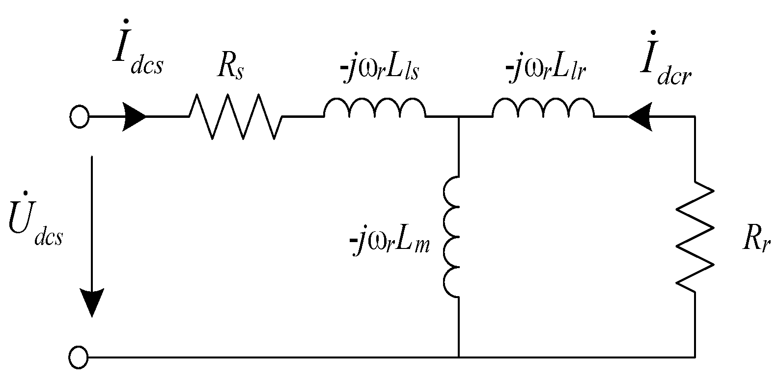
2.1. Stator and Rotor Flux of IGs during Grid Faults

All parameters in this paper are per unit. The stator short-circuit current of the IG is determined by the stator and rotor fluxes when an unsymmetrical fault occurs. The stator and rotor fluxes of IG are not affected by the zero-sequence component of the voltage [13], whereas the forced sinusoidal component is driven only by the positive and negative sequence components of the IG terminal voltage. With the motor convention, the stator voltage equation of the IG under an unsymmetrical fault using a space vector can be written as:

$${\mathit{u}}_s(t)={\mathit{u}}_{1s}(t)+{\mathit{u}}_{2s}(t)={\dot{U}}_{1s}{e}^{j{\mathsf{\omega }}_{s}t}+{\dot{U}}_{2s}{e}^{-j{\mathsf{\omega }}_{s}t}=R_s[{\mathit{i}}_{1s}(t)+{\mathit{i}}_{2s}(t)]+\frac{d}{dt}[{\mathbf{\psi }}_{1s}(t)+{\mathbf{\psi }}_{2s}(t)]$$

(1)

where u_1s(t) and u_2s(t) are the positive and negative voltage space vectors, i_1s(t) and i_2s(t) are the positive and negative current space vectors, R_s is the stator resistance, ψ_1s(t) and ψ_2s(t) are the positive and negative fluxes after faults, ${\dot{U}}_{1s}$ and ${\dot{U}}_{2s}$ are the sequence component phasors of the stator voltage, and ω_s is the synchronous electric angular velocity. When the stator resistance is disregarded, the forced components of the stator flux can be expressed as ψ_1s(t) = ${\dot{U}}_{1s}{e}^{j{\mathsf{\omega }}_{s}t}/j{\mathsf{\omega }}_s$ and ψ_2s(t) = $-{\dot{U}}_{2s}{e}^{-j{\mathsf{\omega }}_{s}t}/j{\mathsf{\omega }}_s$ by solving Equation (1). According to the flux linkage conservation, the post-fault stator flux also contains a DC component. Assuming the normal operation voltage u_s(t) = ${\dot{U}}_s{e}^{j{\mathsf{\omega }}_{s}t}$, then the stator post-fault flux linkage ψ_s(t) of IG can be given as:

$${\mathbf{\psi }}_s(t)=\frac{{\dot{U}}_{1s}}{j{\mathsf{\omega }}_s}{e}^{j{\mathsf{\omega }}_{s}t}-\frac{{\dot{U}}_{2s}}{j{\mathsf{\omega }}_s}{e}^{-j{\mathsf{\omega }}_{s}t}+[\frac{{\dot{U}}_s}{j{\mathsf{\omega }}_s}-(\frac{{\dot{U}}_{1s}}{j{\mathsf{\omega }}_s}-\frac{{\dot{U}}_{2s}}{j{\mathsf{\omega }}_s})]e^{-t/T_s}$$

(2)

where T_s = (L_s − L_m²/L_r)/R_s is the stator time constant, L_m is the excitation inductance, L_s = L_ls + L_m, L_r = L_lr + L_m, and L_ls and L_lr are the leakage inductances of stator and rotor. The post-fault forced flux components in the stator are the steady-state response, and the positive and negative forced components in the rotor can be derived through the steady-state equivalent circuits in Figure 1. The relationship between the rotor current ${\dot{I}}_{1r}$, ${\dot{I}}_{2r}$ and the stator current ${\dot{I}}_{1s}$, ${\dot{I}}_{2s}$ can be expressed as follows:

$${\dot{I}}_{1r}=\frac{-j{\mathsf{\omega }}_s{L}_m{\dot{I}}_{1s}}{R_r/s+j{\mathsf{\omega }}_s{L}_r},{\dot{I}}_{2r}=\frac{j{\mathsf{\omega }}_s{L}_m{\dot{I}}_{2s}}{R_r/(2-s)-j{\mathsf{\omega }}_s{L}_r}$$

(3)

where R_r is the rotor resistance, the rotor slip s = (ω_s − ω_r)/ω_s, and ω_r is the rotor angular velocity. Combining ψ_s(t) = L_si_s(t) + L_mi_r(t) and ψ_r(t) = L_mi_s(t) + L_ri_r(t), the post-fault forced components in the rotor can be calculated as follows:

$$\begin{array}{l}{\mathbf{\psi }}_{1r}(t)=\frac{L_m{R}_r/s\cdot {\mathbf{\psi }}_{1s}(t)}{L_s{R}_r/s+j{\mathsf{\omega }}_s(L_s{L}_r-L_m^2)}={\mathsf{\eta }}_{1rs}(s){\mathbf{\psi }}_{1s}(t)\\ {\mathbf{\psi }}_{2r}(t)=\frac{L_m{R}_r/(2-s)\cdot {\mathbf{\psi }}_{2s}(t)}{L_s{R}_r/(2-s)-j{\mathsf{\omega }}_s(L_s{L}_r-L_m^2)}={\mathsf{\eta }}_{2rs}(s){\mathbf{\psi }}_{2s}(t)\end{array}$$

(4)

With a 3MW IG (the parameters are given in [18]) as an example, Figure 2 illustrates the amplitude and phase characteristics of the positive and negative sequence correlation coefficients η_1rs and η_2rs in Equation (4) between the stator and rotor flux. The amplitude of η_1rs is near 1.0 when the rotor slip is small in the normal operation [2]. When the slip drops to −0.1 during the fault, the amplitude of η_1rs will decrease by 90%, as shown in Figure 2. This decrease indicates that a small slip change has a significant influence on the positive sequence forced rotor flux in the rotor. Therefore the slip change should be taken into consideration in the rotor flux calculation.

The negative sequence flux component in rotor windings induced by the stator negative sequence forced flux can be neglected, because η_2rs is near zero under the different rotor slips for a fixed-speed IG in Figure 2a. However, there are still negative sequence short-circuit currents of IGs caused by the grid negative sequence voltages, especially, the negative sequence current of a variable-speed IG is mainly influenced by the control structures and objectives in its machine side and line side converters [19]. The rotor resistance of a variable-speed IG will increase significantly after its crowbar protection activation during grid faults and the magnitude of η_2rs will stay in the range of 0.2–0.3 pu under different rotor slips, as shown in Figure 2b. In this figure, the rotor resistance rises to 25 times that of the fixed-speed IG, and so a non-ignorable flux component in the rotor windings of a variable-speed IG can be generated by the negative sequence component of the stator flux. Besides the coupling differences of flux forced components between fixed-speed and variable-speed IGs, the decay time constant of the rotor flux DC component, T_r = (L_r − L_m²/L_s)/R_r, will also be changed by increase in rotor resistance of variable-speed IGs during a grid fault.

The stator flux ψ_s(t) has both the positive and negative sequence forced components ψ_1s(t) and ψ_2s(t) and the DC component ψ_dcs(t) in Equation (2). The reverse rotation flux with the rotor speed will be generated in the rotor windings because of ψ_dcs(t) cutting the rotor windings. The stator flux DC component is difficult to analyze in the stator reference frame, but it can be discussed in the rotor side by the frequency transformation [2]. The equivalent circuit in the rotor reference frame for the stator flux DC component is shown in Figure 3, where ${\dot{I}}_{dcs}$ and ${\dot{I}}_{dcr}$ are the DC components of the stator and rotor currents, and ${\dot{U}}_{dcs}$ is a virtual voltage caused by the stator flux DC component. With the relationship of the stator current ${\dot{I}}_{dcs}$ and the rotor current ${\dot{I}}_{dcr}$ in Figure 3, the rotor flux component ψ_dcr(t) caused by the stator flux DC component ψ_dcs(t) can be obtained as:

$${\mathbf{\psi }}_{dcr}(t)=\frac{L_m{R}_r\cdot {\mathbf{\psi }}_{dcs}(t)}{L_s{R}_r-\mathrm{j}{\mathsf{\omega }}_s(1-s)(L_s{L}_r-L_m^2)}={\mathsf{\eta }}_{dcrs}(s){\mathbf{\psi }}_{dcs}(t)$$

(5)

The amplitude and phase characteristics of the DC component correlation coefficient η_dcrs in Equation (5) between the stator and rotor fluxes are shown in Figure 4. The reverse rotation flux component ψ_dcr(t) in the rotor windings of a fixed-speed IG is approximately zero because of its small rotor resistance. Meanwhile, the amplitude changing range of η_dcrs for a variable-speed IG is from 0.4 pu to 0.6 pu as the rotor slips increase. The rotor flux of variable-speed IG will also appear as a significant reverse rotation component in the rotor flux.

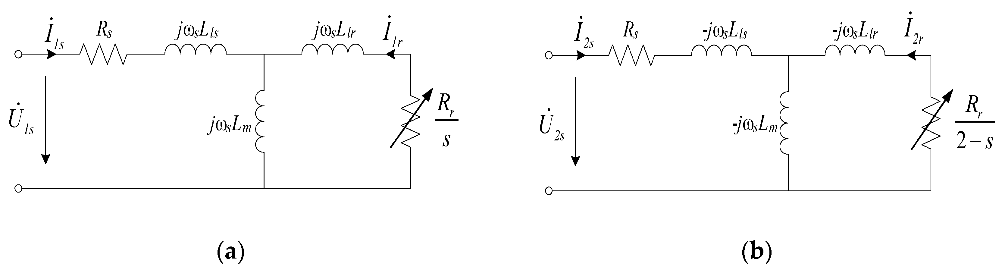
2.2. Sequence Component Current Model of Fixed-Speed IGs

Assuming the initial slip of a fixed-speed IG is s₀ before the short-circuit fault occurrs, the rotor flux linkage ψ_r(t) of the fixed-speed IG in the stator reference frame is derived as in Equation (6) according to the flux linkage conservation:

$${\mathbf{\psi }}_r(t)={\mathsf{\eta }}_{1rs}(s)\frac{{\dot{U}}_{1s}}{j{\mathsf{\omega }}_s}{e}^{j{\mathsf{\omega }}_{s}t}+{\mathsf{\eta }}_{1rs}(s_0)\frac{{\dot{U}}_s-{\dot{U}}_{1\text{s}}}{j{\mathsf{\omega }}_s}{e}^{-t/T_r}{e}^{j{\mathsf{\omega }}_{r}t}$$

(6)

where T_r = (L_r − L_m²/L_s)/R_r is the rotor time constant. With Equations (2) and (6) substituted into i_s(t) = (L_rψ_s − L_mψ_r)/(L_sL_r − L_m²), the general expression for the post-fault stator short-circuit current of a fixed-speed IG can be given as:

$$\begin{array}{l}{\mathit{i}}_s(t)=\frac{1}{L_s{L}_r-L_m^2}\{[L_r-L_m{\mathsf{\eta }}_{1rs}(s)]\frac{{\dot{U}}_{1s}}{j{\mathsf{\omega }}_{\mathrm{s}}}{e}^{j{\mathsf{\omega }}_{s}t}-L_m{\mathsf{\eta }}_{1rs}(s_0)\cdot \frac{{\dot{U}}_s-{\dot{U}}_{1s}}{j{\mathsf{\omega }}_s}{e}^{-t/T_r}{e}^{j{\mathsf{\omega }}_{r}t}\}\\ +\frac{L_r}{L_s{L}_r-L_m^2}\frac{{\dot{U}}_{2\text{s}}}{-j{\mathsf{\omega }}_s}{e}^{-j{\mathsf{\omega }}_{s}t}+\frac{L_r}{L_s{L}_r-L_m^2}[\frac{{\dot{U}}_s}{j{\mathsf{\omega }}_s}-(\frac{{\dot{U}}_{1s}}{j{\mathsf{\omega }}_s}-\frac{{\dot{U}}_{2s}}{j{\mathsf{\omega }}_s})]e^{-t/T_s}\end{array}$$

(7)

The short-circuit current of the fixed-speed IG is composed of three components. The first component is the steady periodic component, which includes both positive and negative components. The second component decays exponentially with the time constant T_r and rotates with ω_r in the stator reference frame because of the natural rotor flux. The third component is the DC component decaying exponentially with the time constant T_s because of the natural stator flux. Given that the neutral point of a distribution network is commonly not grounded or grounded by arc-suppression coil, the zero sequence is not considered here. When a short-circuit fault occurs in distribution networks with multiple IGs, the short-circuit currents of IGs inject into the distribution network in the form of a variable current source based on symmetrical components, and the DC component is not within the symmetrical network.

The change law of the short-circuit current with time and the relation between the current and terminal voltage sequence components of IG can be determined by Equation (7). With a terminal three-phase short circuit, the rotor speed after 10 cycles is less than 1.10 when a rated torque is given [20]. Thus the AC component of the short-circuit current rotating with ω_r can be considered a synchronous frequency component. Assuming the slips of m sets of fixed-speed IGs are s_i (i = 1,2,…,m), the positive and negative sequence phasors of the short-circuit current for the ith fixed-speed IG can be derived as in Equations (8) and (9):

$${\dot{I}}_{1si}=\frac{1}{L_{si}{L}_{ri}-L_{mi}^2}\{[L_{ri}-L_{mi}{\mathsf{\eta }}_{1rsi}(s_i)]\frac{{\dot{U}}_{1si}}{j{\mathsf{\omega }}_s}-L_{mi}{\mathsf{\eta }}_{1rsi}(s_{i0})\frac{{\dot{U}}_{si}-{\dot{U}}_{1si}}{j{\mathsf{\omega }}_s}{e}^{-t/T_{ri}}\}$$

(8)

$${\dot{I}}_{2si}=\frac{L_{ri}}{L_{si}{L}_{ri}-L_{mi}^2}\frac{{\dot{U}}_{2si}}{-j{\mathsf{\omega }}_s}$$

(9)

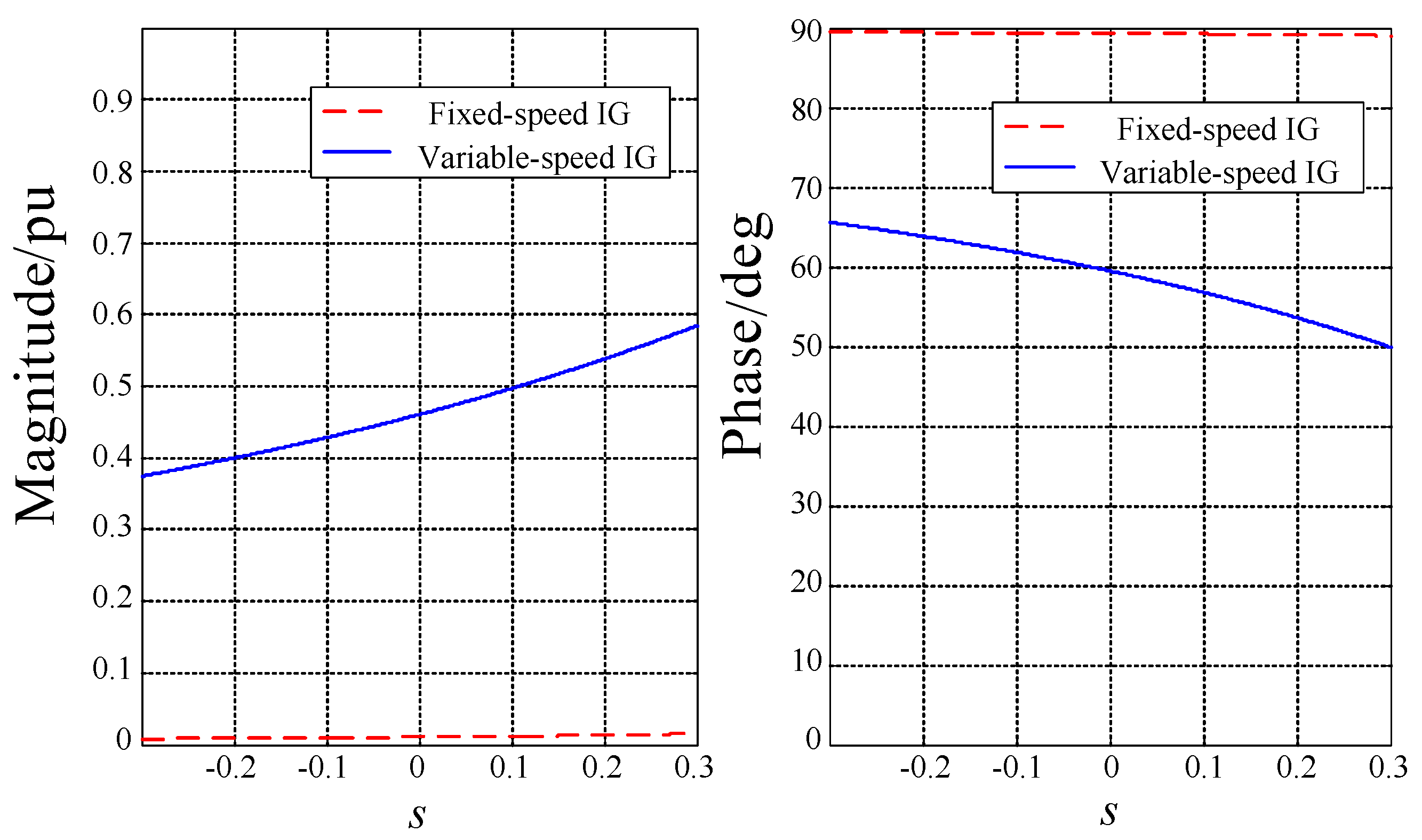
2.3. Sequence Component Current Model of Variable-Speed IGs

Besides considering the effect of positive sequence forced component ψ_1s(t) in the stator flux, the post-fault rotor flux of the variable-speed IG has to include the flux components produced by the negative sequence forced component ψ_2s(t) and the DC component ψ_dcs(t). According to the flux linkage conservation before and after a short-circuit fault occurs, the post-fault rotor flux ψ_r(t) of the variable-speed IG in the stator reference frame can be given as:

$$\{\begin{array}{ccc}\hfill {\mathbf{\psi }}_r(t)& =& {\mathsf{\eta }}_{1rs}(s)\frac{{\dot{U}}_{1s}}{j{\mathsf{\omega }}_s}{e}^{j{\mathsf{\omega }}_{s}t}-{\mathsf{\eta }}_{2rs}(s)\frac{{\dot{U}}_{2s}}{j{\mathsf{\omega }}_s}{e}^{-j{\mathsf{\omega }}_{s}t}+{\mathsf{\eta }}_{dcrs}(s)[\frac{{\dot{U}}_s}{j{\mathsf{\omega }}_s}-(\frac{{\dot{U}}_{1s}}{j{\mathsf{\omega }}_s}-\frac{{\dot{U}}_{2s}}{j{\mathsf{\omega }}_s})]e^{-t/T_s}+{\mathbf{\psi }}_{r0}{e}^{-t/T_r}{e}^{j{\mathsf{\omega }}_{r}t}\hfill \\ \hfill {\mathbf{\psi }}_{r0}& =& {\mathsf{\eta }}_{1rs}(s_0)\frac{{\dot{U}}_s-{\dot{U}}_{1s}}{j{\mathsf{\omega }}_s}+{\mathsf{\eta }}_{2rs}(s_0)\frac{{\dot{U}}_{2s}}{j{\mathsf{\omega }}_s}-{\mathsf{\eta }}_{dcrs}(s_0)[\frac{{\dot{U}}_s}{j{\mathsf{\omega }}_s}-(\frac{{\dot{U}}_{1s}}{j{\mathsf{\omega }}_s}-\frac{{\dot{U}}_{2s}}{j{\mathsf{\omega }}_s})]\hfill \end{array}$$

(10)

The stator current can be obtained as i_s(t) = (L_rψ_s − L_mψ_r)/(L_sL_r − L_m²) through the relationships among the flux and current in the stator and rotor windings. Combined with the formulas of ψ_s(t) and ψ_r(t), the short-circuit current of a variable-speed IG can be written as:

$$\begin{array}{l}{\mathit{i}}_{\mathrm{s}}(t)=\frac{1}{L_s{L}_r-L_m^2}\left\{[L_r-L_m{\mathsf{\eta }}_{1rs}(s)]\frac{{\dot{U}}_{1s}}{j{\mathsf{\omega }}_s}{e}^{j{\mathsf{\omega }}_{s}t}-L_m{\mathbf{\psi }}_{r0}{e}^{-t/T_r}{e}^{j{\mathsf{\omega }}_{r}t}\right\}\\ +\frac{L_r-L_{\mathrm{m}}{\mathsf{\eta }}_{2\text{rs}}(s)}{L_s{L}_r-L_m^2}\frac{{\dot{U}}_{2s}}{-j{\mathsf{\omega }}_s}{e}^{-j{\mathsf{\omega }}_{s}t}+\frac{L_r-L_m{\mathsf{\eta }}_{dcrs}(s)}{L_s{L}_r-L_m^2}[\frac{{\dot{U}}_s}{j{\mathsf{\omega }}_s}-(\frac{{\dot{U}}_{1s}}{j{\mathsf{\omega }}_s}-\frac{{\dot{U}}_{2s}}{j{\mathsf{\omega }}_s})]e^{-t/T_s}\end{array}$$

(11)

The positive sequence steady component of the short-circuit current of variable-speed IG is the same as that of fixed-speed IG, but the positive sequence steady component, transient decay AC component rotoring with ω_r, and DC component are different from those in Equation (7) because of the nonignorable flux correlation coefficients η_2rs and η_dcrs In consideration of the AC component rotoring with ω_r as a synchronous frequency component, the positive and negative sequence phasors of the short-circuit current for the ith variable-speed IG can be derived as follows:

$${\dot{I}}_{1si}=\frac{1}{L_{si}{L}_{ri}-L_{mi}^2}\left\{[L_{ri}-L_{mi}{\mathsf{\eta }}_{1rsi}(s_i)]\frac{{\dot{U}}_{1si}}{j{\mathsf{\omega }}_s}-L_{mi}\left[{\mathsf{\eta }}_{1rsi}(s_{i0})\frac{{\dot{U}}_{si}-{\dot{U}}_{1si}}{j{\mathsf{\omega }}_s}+{\mathsf{\eta }}_{2rsi}(s_{i0})\frac{{\dot{U}}_{2si}}{j{\mathsf{\omega }}_s}-{\mathsf{\eta }}_{dcrsi}(s_{i0})\left(\frac{{\dot{U}}_{si}}{j{\mathsf{\omega }}_s}-\frac{{\dot{U}}_{1si}}{j{\mathsf{\omega }}_s}+\frac{{\dot{U}}_{2si}}{j{\mathsf{\omega }}_s}\right)\right]e^{-t/T_{ri}}\right\}$$

(12)

$${\dot{I}}_{2si}=\frac{L_{ri}-L_{mi}{\mathsf{\eta }}_{2rsi}(s_i)}{L_{si}{L}_{ri}-L_{mi}^2}\frac{{\dot{U}}_{2si}}{-j{\mathsf{\omega }}_s}$$

(13)

According to the interaction among the stator short-circuit current, network equation and rotor movement equation, the terminal voltage and slip can be updated iteratively in each data window during the fault. The calculation process is similar with that of the simulation software. The IGs are represented by the analytical expressions including Equations (8), (9), (12) and (13) in the proposed method, while the simulation software adopts the fifth-order differential-algebraic equations as the model of IGs. Then the time series for the positive and negative sequence components of the short-circuit current can be determined based on the dynamic phasor and analytical expression during the fault process from sub-transient to steady-state.

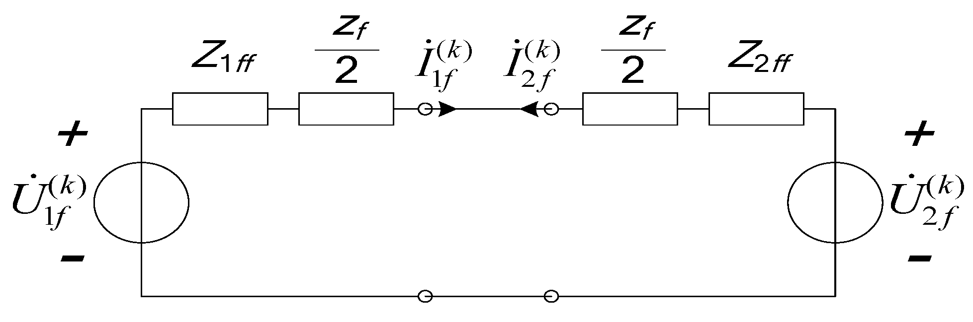
3. Coupling Relationship between Short-Circuit Current of IGs and the Distribution Network

When the integrated capacity of IGs is small, the terminal voltages of IGs will drop to a steady-state value as soon as the fault occurs in a distribution network [13,14,15]. However, the terminal voltages will be significantly changed by their own short-circuit current injections in a distribution network with high permeability of IGs. In this case, the coupling between short-circuit currents of IGs and distribution network have to be considered. A distribution network with a short-circuit capacity of 240 MW is analyzed, and the short-circuit ratio (SCR) [21] between IG and network is 80. The dynamic simulation and calculation results of a fixed-speed IG with a three-phase short-circuit fault at the end of the feeder downstream are shown in Figure 5, where ε is the relative error of the calculation results. By setting the impedance of the downstream feeder equal to the short-circuit impedance of the network, the voltage dip magnitude at the generator terminals during a fault can be fixed to a proportion p = 0.5 (the voltage changes from ${\dot{U}}_s$ to $p{\dot{U}}_s$, where p is the proportion of the post-fault voltage versus the pre-fault voltage), the rotor speed increases in a linear manner with a slope of (p² − 1)T_m/(2H), where T_m = −1.0 is the mechanical torque and H = 5.04 s is the inertia constant.

The short-circuit current can be calculated by substituting the pre-fault and post-fault terminal voltages and slip variation of IGs into Equation (8). The calculation results under the variable slip and fixed slip (including both the initial slip s₀ = −0.0051 pu and zero slip) are shown in Figure 5. The calculation error of fixed slip increases with time. The calculation accuracy with initial slip is above that of zero slip, although its relative error can be over 10%. The comparison results show that the calculation results with variable slip is much closer to the simulation results.

When a phase B to phase C fault occurs at the end of the feeder downstream, the sequence components of the terminal voltage are ${\dot{U}}_{1s}=3p/2{\dot{U}}_s$ and ${\dot{U}}_{2s}=p/2{\dot{U}}_s$, and the rotor speed increases with the slope of (5p²/2 − 1)T_m/(2H), where T_m = −0.5. Figure 6 shows the sequence components of the short-circuit of fixed-speed and variable-speed IGs in the case of two-phase fault. The positive and negative sequence components of short-circuit current of IG are extracted by a sequence filter based on the second-order generalized integrators [22]. The output of filter is the instantaneous waveform of positive and negative sequence current, and then the RMS value of instantaneous waveform can be computed through a RMS block.The negative sequence component I_2s of fixed-speed IG reaches its steady-state value directly and doesn’t change with the slip in Figure 6a, while I_2s of variable-speed IG decreases with the increase of fault duration because of the rising rotor speed in Figure 6b.

The steady-state short-circuit currents of variable-speed IGs in Figure 6b are less than that of fixed-speed IGs because of the offsetting effect from the short-circuit currents caused by the positive and negative sequence forced fluxes in rotor windings, which are markedly influenced by the rotor resistance and the rotor speed. For the steady-state short-circuit currents, the signs of η_1rs and η_2rs are minus in Equations (12) and (13) where the change of η_1rs with rotor slip becomes slow and the magnitude of η_2rs stays in the range of 0.2–0.3 pu due to the rising of rotor resistance of variable-speed IGs. The calculation results of fixed initialand zero slips can not match the real trend of I_2s of variable-speed IG during a grid fault. Although the calculation error with a fixed initial slip (s₀ = −0.0023 pu) is slightly reduced because of the smaller rotor slip differences compared to that of zero slip, the errors are still larger than that with a variable slip in both cases of fixed-speed and variable-speed IGs.

Figure 7 shows the terminal voltage and short-circuit current response of fixed-speed IGs with a three-phase fault at the end of feeder downstream when an IG, four IGs, and eight IGs are integrated into a distribution network with a short-circuit capacity of 240 MW separately. Furthermore, the peak values I_1sp of the short-circuit current of fixed-speedand variable-speed IGs under different SCRs are shown in the figure. A large difference is observed between the calculation results of fixed-speed IGs using Equation (8) without considering the transient variation of terminal voltage and the simulation results with a small SCR. According to the variation of I_1sp with SCR, it is unnecessary to consider the effect of the short-circuit current of IGs on their terminal voltage when SCR ≥ 20 for fixed-speed IGs and SCR ≥ 40 for variable-speed IGs. However, the current of IGs is determined by both the transient characteristics of the IG generator and the power system network equations when SCR < 20 for fixed-speed IGs and SCR < 40 for variable-speed IGs.

When a short-circuit fault occurs at a distribution network, the surge current in the stator winding is driven mainly by the stator transient DC flux linkage. At the same time, the transient AC component of the stator current is produced by the rotor flux linkage. The injection of short-circuit current changes the distribution of nodal voltages in the distribution network, and the terminal voltage of IGs changes with the decaying current, and then affects the short-circuit current in reverse. Therefore, besides the slip change, the interaction of the injection current of IGs and the network equations for short-circuit calculation of a multi-IG system must be thoroughly considered.

The coupling relation between the short-circuit current of IG and the distribution network is shown in Figure 8, where only the current source model of IG (at bus i) is given. Bus 1 is the main source node of distribution network, ${\dot{E}}_s$, Z_1s and Z_2s are the voltages (i.e., the positive and negative sequence of the main source), ${\dot{U}}_{1f}$, ${\dot{U}}_{2f}$, ${\dot{I}}_{1f}$, and ${\dot{I}}_{2f}$ are the sequence components of voltage and current at the fault bus f. When a fault occurs at bus f, the initial short-circuit current can be determined by the initial conditions, and then the voltage can be updated in the next step by substituting the current into network equations. Meanwhile, the electromagnetic power is calculated to update the slip.

The terminal voltage and slip can be considered constant in the step because the iterative step is very small. At the initial time of fault, the initial value of short-circuit current of IGs can be obtained according to the unchanged transient potentialof IGs at the fault moment, and their terminal voltages during the first iterative step can also be determined by combining the network equations and the short-circuit current injection of IGs. Then the voltages of the last iterative step can be substituted into Equations (8) and (9) for a fixed-speed IG, as well as Equations (12) and (13) for a variable-speed IG, to achieve the short-circuit currents of IGs at the next iterative step. The positive sequence currents of fixed-speed and variable-speed IGs exponentially decayin terms of the rotor time constant in Equations (8) and (12), whereas the negative sequence current of variable-speed IG changes only with the rotor slip in Equation (13). The terminal voltages and rotor slips can be calculated at this iterative step and used to determine the short-circuit currents of IGs by the equations at the next iterative step. The method to determine the sequence components of short-circuit current using the current source model of IGs will be given in the next section.

4. Short-Circuit Calculation of the Multi-IG Network

4.1. Initial Value Calculation for Short-Circuit CurrentSequence Components of IGs

Substituting ψ_s(t)/dt and dψ_r(t)/dt, which are determined by the stator and rotor voltage equations, into the differential of i_s = [L_rψ_s(t) − L_mψ_r(t)]/(L_sL_r − L_m²) as:

$$\frac{L_s{L}_r-L_m^2}{L_r}\frac{d{\mathit{i}}_s(t)}{dt}=\frac{d{\mathbf{\psi }}_s(t)}{dt}-\frac{L_m}{L_r}\frac{d{\mathbf{\psi }}_r(t)}{dt}={\mathit{u}}_s(t)-R_s{\mathit{i}}_s(t)-\frac{L_m}{L_r}[j{\mathsf{\omega }}_r{\mathbf{\psi }}_r(t)-R_r{\mathit{i}}_r(t)]$$

(14)

Equation (14) can be modified using i_r(t) = [L_sψ_r(t) − L_mψ_s(t)]/(L_sL_r − L_m²). The expression of u_s(t) can be then written as:

$${\mathit{u}}_s(t)=R_s{\mathit{i}}_s(t)+\frac{L_s{L}_r-L_m^2}{L_r}\frac{d{\mathit{i}}_s(t)}{dt}+\frac{L_m}{L_r}[(j{\mathsf{\omega }}_r-\frac{R_r{L}_s}{L_s{L}_r-L_m^2}){\mathbf{\psi }}_r(t)+\frac{R_r{L}_m}{L_s{L}_r-L_m^2}{\mathbf{\psi }}_s(t)]$$

(15)

The fluxes ψ_s(t) and ψ_r(t) remain unchanged at the moment the fault occurs. Thus, the third part of Equation (15) can be defined as the transient equivalent potential of IG. Assume there are m sets of IGs in the distribution network, and the integrated buses of IGs are from bus 2 to bus m + 1. The transient equivalent potential of the ith IG can be described as follows:

$${\dot{E}}_{si}^{\prime }={\dot{U}}_{si}-Z_{1si}^{\prime }{\dot{I}}_{\mathrm{s}i}={\dot{U}}_{si}-(R_{si}+j{\mathsf{\omega }}_s\frac{L_{si}{L}_{ri}-L_{mi}^2}{L_{ri}}){\dot{I}}_{si}$$

(16)

where $Z_{1si}^{\prime }$ is the positive transient impedance of the ith IG. Given that the three phase quantities form a balanced system during normal operation, the pre-fault voltage and current can be calculated using the Newton-Raphson method, then the transient equivalent potential can be determined. With the iteration step for short-circuit calculation defined as Δt = T/2 (T = 0.02s), the initial value of the short-circuit current can be determined by the unchanged transient potential at the first step. Adding the positive and negative impedances $Z_{1si}^{\prime }=Z_{2si}^{\prime }$ of IGs into the original positive and negative matrix Z₁ and Z₂ of the network to form the node-impedance matrixes Z₁′ and Z₂′ of n × n order. The normal operation voltage of each node:

$${\dot{U}}^{(0)}={{\rm Z}}_1^{\prime }{\dot{I}}^{(0)}={{\rm Z}}_1^{\prime }{[{\dot{I}}_1,{\dot{I}}_2^{(0)},\cdots ,{\dot{I}}_{m+1}^{(0)},0,\cdots ,0]}^T$$

(17)

where ${\dot{I}}_1={\dot{E}}_s/Z_{1s}$ and ${\dot{I}}_i^{(0)}={\dot{E}}_{si}^{\prime }/Z_{1si}^{\prime }$ are the equivalent current of the main source and the Norton circuit of the ith IG respectively. The normal voltages of each node are equal to the pre-fault voltages of each node in the network because the transient equivalent potential of IGs remains unchanged at the first step. Taking a phase B to phase C fault at bus f for an example, the sequence components of the short-circuit current at the fault bus at the first iterative step can be calculated as:

$${\dot{I}}_{1f}^{(1)}=-{\dot{I}}_{2f}^{(1)}=\frac{{\dot{U}}_f^{(1)}}{Z_{1ff}^{\prime }+Z_{2ff}^{\prime }+z_f}=\frac{{\dot{U}}_f^{(0)}}{Z_{1ff}^{\prime }+Z_{2ff}^{\prime }+z_f}$$

(18)

The voltage phasors of each node in the positive and negative sequence fault component networks can be derived as Equation (19) using the superposition principle in fault analysis:

$$\begin{array}{l}\Delta {\dot{U}}_1^{(1)}={[Z_{11f}^{\prime },\cdots ,Z_{1if}^{\prime }\cdots ,Z_{1nf}^{\prime }]}^T(-{\dot{I}}_{1f}^{(1)})\\ \Delta {\dot{U}}_2^{(1)}={[Z_{21f}^{\prime },\cdots ,Z_{2if}^{\prime }\cdots ,Z_{2nf}^{\prime }]}^T(-{\dot{I}}_{2f}^{(1)})\end{array}$$

(19)

The post-fault voltage phasors are ${\dot{U}}_1^{\prime (1)}={\dot{U}}^{(1)}+\Delta {\dot{U}}_1^{(1)}$ and ${\dot{U}}_2^{\prime (1)}=\Delta {\dot{U}}_2^{(1)}$, and the initial values of the positive and negative sequence short-circuit current at the first step are given as:

$${\dot{I}}_{1si}^{(1)}(0)=\frac{{\dot{U}}_{1i}^{\prime (1)}-{\dot{E}}_{\mathrm{s}i}^{\prime }}{Z_{1\mathrm{s}i}^{\prime }},{\dot{I}}_{2\text{s}i}^{(1)}(0)=\frac{{\dot{U}}_{2i}^{\prime (1)}}{Z_{2\text{s}i}^{\prime }}$$

(20)

Given that the sequence components of the terminal voltage and the slip are unchanged at each step, the positive sequence component of the short-circuit current decays exponentially with the time constant T_r, while the negative component is unchanged according to Equations (8), (9), (12), and (13), The RMS of the negative sequence current in the first Δt is ${[I_{2\mathrm{s}i}^{(1)}]}_{\text{rms}}=I_{2\mathrm{s}i}^{(1)}(\Delta t)=I_{2\mathrm{s}i}^{(1)}(0)$. The RMS of the positive sequence short-circuit current at the end of the first step can be derived by substituting ${\dot{U}}_{1i}^{\prime (1)}$ and s_i⁽¹⁾ = s_i0 into Equations (8) and (12). The positive sequence component of the short-circuit current at the first step is given as:

$$I_{1\text{s}i}^{(1)}(t)=\frac{[I_{1\mathrm{s}i}^{(1)}(\Delta t)-I_{1\mathrm{s}i}^{(1)}(0)e^{-\Delta t/T_{\mathrm{r}i}}]I_{1\mathrm{s}i}^{(1)}(\Delta t)}{I_{1\mathrm{s}i}^{(1)}(\Delta t)(1-e^{-\Delta t/T_{\mathrm{r}i}})}+\frac{[I_{1\mathrm{s}i}^{(1)}(0)-I_{1\mathrm{s}i}^{(1)}(\Delta t)]e^{-t/T_{\mathrm{r}i}}}{1-e^{-\Delta t/T_{\mathrm{r}i}}}=A_i^{(1)}{I}_{1\mathrm{s}i}^{(1)}(\Delta t)+B_i^{(1)}[I_{1\mathrm{s}i}^{(1)}(0)-I_{1\mathrm{s}i}^{(1)}(\Delta t)]e^{-t/T_{\mathrm{r}i}}$$

(21)

The first point of RMS values cannot reflect the maximum value of instantaneous waveform in simulation because the RMS computation has a time lag, while the calculation results of RMS currents are widely used to identify the rating of electrical equipment, the selection of fuses and the setting of protective devices. The RMS of the positive sequence short-circuit current at the first step can be derived as follows: (the process is presentedin detail in Appendix A)

$${[I_{1\mathrm{s}i}^{(1)}]}_{rms}=\sqrt{\begin{array}{l}{[A_i^{(1)}{I}_{1\mathrm{s}i}^{(1)}(\Delta t)]}^2+\frac{T_{\mathrm{r}i}}{T}{B}_i^{(1)}[I_{1\mathrm{s}i}^{(1)}(0)-I_{1\mathrm{s}i}^{(1)}(\Delta t)]\{4A_i^{(1)}{I}_{1\mathrm{s}i}^{(1)}(\Delta t)\cdot \\ [1-e^{-T/(2T_{\mathrm{r}i})}]+B_i^{(1)}[I_{1\mathrm{s}i}^{(1)}(0)-I_{1\mathrm{s}i}^{(1)}(\Delta t)](1-e^{-T/T_{\mathrm{r}i}})\}\end{array}}$$

(22)

4.2. Short-Circuit CurrentSequence Components of IGs during Grid Faults

When a fault occurs in the network with multiple IGs, the short-circuit currents of IGs inject into the sequence network in the form of a dynamic current source based on its terminal voltage. The instantaneous electromagnetic power of IGs is made up of DC and double frequency components if the terminal voltage and current of the IGs contain both positive and negative components. The average of the double-frequency component in a half cycle is zero, and so the average of the electromagnetic power at step k − 1 can be derived as Equation (23) by the terminal voltage and short-circuit current of the ith IG:

$$P_{\mathrm{e}i}^{(k-1)}=U_{1i}^{\prime (k-1)}{[I_{1\mathrm{s}i}^{(k-1)}]}_{rms}\cos {\mathsf{\phi }}_{1i}^{(k-1)}+U_{2i}^{\prime (k-1)}{[I_{2\mathrm{s}i}^{(k-1)}]}_{rms}\cos {\mathsf{\phi }}_{2i}^{(k-1)}$$

(23)

where ϕ_1i^(k−1) is the positive power factor angle ${\dot{U}}_{1i}^{\prime (k-1)}$ leading $[{\dot{I}}_{1\text{s}i}^{(k-1)}(\Delta t)+{\dot{I}}_{1\text{s}i}^{(k-1)}(0)]$/2, and ϕ _2i^(k−1) is the negative sequence power factor angle ${\dot{U}}_{2i}^{\prime (k-1)}$ leading ${\dot{I}}_{2\mathrm{s}i}^{(k-1)}(0)$. Solving the rotor motion equation of IGs with the rectangular integral method can derive the slip of the ith IG at step k as:

$$s_i^{(k)}=s_i^{(k-1)}-\frac{\Delta t}{2H_i}[\frac{P_{\mathrm{e}i}^{(k-1)}}{1-s_i^{(k-1)}}-T_{\mathrm{m}i}]$$

(24)

According to the currents ${\dot{I}}_{1\text{s}i}^{(k-1)}(\Delta t)$ and ${\dot{I}}_{2\mathrm{s}i}^{(k-1)}(\Delta t)$ of IGi at the end of step k − 1, the node voltage of the normal network at step k can be updated iteratively as:

$$\begin{array}{l}{\dot{U}}_1^{(k)}={{\rm Z}}_1{\dot{I}}_{1\mathrm{s}i}^{(k-1)}(\Delta t)={{\rm Z}}_1{[{\dot{I}}_1,{\dot{I}}_{1\mathrm{s}i}^{(k-1)}(\Delta t),\cdots ,{\dot{I}}_{1\mathrm{s}(m+1)}^{(k-1)}(\Delta t),0,\cdots ,0]}^T\\ {\dot{U}}_2^{(k)}={{\rm Z}}_2{\dot{I}}_{2\mathrm{s}i}^{(k-1)}(\Delta t)={{\rm Z}}_2{[0,{\dot{I}}_{2\mathrm{s}i}^{(k-1)}(\Delta t),\cdots ,{\dot{I}}_{2\mathrm{s}(m+1)}^{(k-1)}(\Delta t),0,\cdots ,0]}^T\end{array}$$

(25)

The multiple IGs are equivalent to the current sources, and Z₁ and Z₂ are the original impedance matrixes of the distribution network. Owing to the negative short-circuit current of IGs injecting into the network, the voltage at the fault node f in the normal network contains a negative sequence voltage component. The sequence components of the short-circuit current at fault node f under a different fault type can be derived using the boundary conditions at the fault node and the composite sequence network with negative sequence voltage.

Taking a phase B to phase C fault through the impedance z_f at the fault node f as an example, as shown in Figure 9, the sequence components of the short-circuit current at fault node f at step k can be expressed as:

$${\dot{I}}_{1f}^{(k)}=-{\dot{I}}_{2f}^{(k)}=\frac{{\dot{U}}_{1f}^{(k)}-{\dot{U}}_{2f}^{(k)}}{Z_{1ff}+Z_{2ff}+z_f}$$

(26)

The post-fault voltage phasors of each node in the positive and negative sequence fault component network at step k are as follows:

$$\begin{array}{l}\Delta {\dot{U}}_1^{(k)}={[Z_{11f},\cdots ,Z_{1if}\cdots ,Z_{1nf}]}^T(-{\dot{I}}_{1f}^{(k)})\\ \Delta {\dot{U}}_2^{(k)}={[Z_{21f},\cdots ,Z_{2if}\cdots ,Z_{2nf}]}^T(-{\dot{I}}_{2f}^{(k)})\end{array}$$

(27)

The positive and negative sequence components of node voltages in the distribution network at step k can be calculated as ${\dot{U}}_1^{\prime (k)}={\dot{U}}_1^{(k)}+\Delta {\dot{U}}_1^{(k)}$ and ${\dot{U}}_2^{\prime (k)}={\dot{U}}_2^{(k)}+\Delta {\dot{U}}_2^{(k)}$ by combining Equations (25) and (27). Subsequently, the sequence components of the short-circuit current at step k can be obtained using ${\dot{U}}_{1i}^{\prime (k)}$, s_i^(k), and ${\dot{U}}_{2i}^{\prime (k)}$.

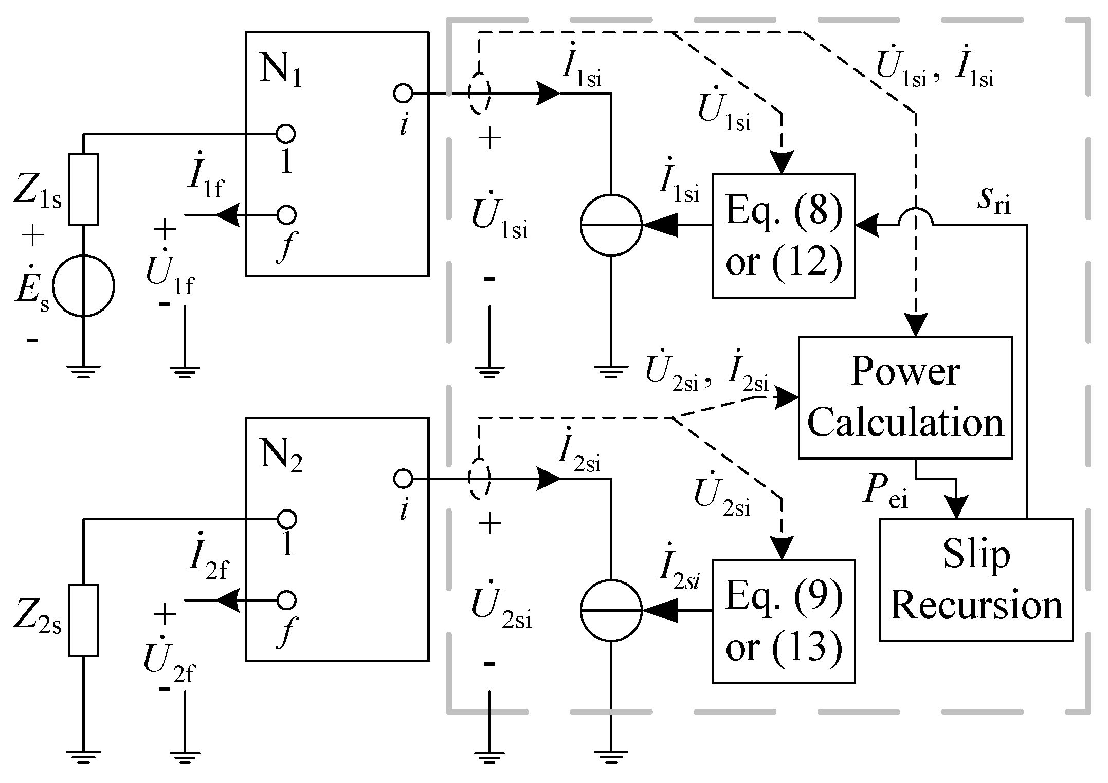
4.3. Procedure of Short-Circuit Calculation

When a fault occurs at node f, the procedure for the short-circuit calculation of the distribution network is summarized as follows:

• Step 1: Form the original matrixes Z₁ and Z₂ of the pre-fault network without IGs, determine the pre-fault voltage ${\dot{U}}_{\mathrm{s}i}$ and stator current ${\dot{I}}_{\mathrm{s}i}$ of each IG according to the mechanical torque during normal operation, and solve Equation (16) to obtain ${\dot{E}}_{\mathrm{s}i}^{\prime }$.
• Step 2: Add $Z_{1\text{s}i}^{\prime }$ and $Z_{2\mathrm{s}i}^{\prime }$ to Z₁ and Z₂ to form the matrixes Z₁′ and Z₂′, obtain ${\dot{U}}^{(1)}$ by Equation (17) and ${\dot{U}}^{(1)}={\dot{U}}^{(0)}$, and then determine ${\dot{I}}_{1f}^{(1)}$ and ${\dot{I}}_{2f}^{(1)}$ according to the fault node and type.
• Step 3: Solve Equation (19) to obtain $\Delta {\dot{U}}_1^{(1)}$ and $\Delta {\dot{U}}_2^{(2)}$, determine ${\dot{U}}_1^{\prime (1)}$ and ${\dot{U}}_2^{\prime (2)}$, and solve Equation (20) to obtain ${\dot{I}}_{1\mathrm{s}i}^{(1)}(0)$ and ${\dot{I}}_{2\mathrm{s}i}^{(1)}(0)$.
• Step 4: Solve Equation (8) for a fixed-speed IG, Equation (12) for a variable-speed IG with ${\dot{U}}_{1i}^{\prime (1)}$ and s_i⁽¹⁾ to obtain ${\dot{I}}_{1\text{s}i}^{(1)}(\Delta t)$, determine the RMS of the positive and negative sequence components ${[I_{1\mathrm{s}i}^{(1)}]}_{rms}$ and ${[I_{2\mathrm{s}i}^{(1)}]}_{rms}$, set ${\dot{U}}_{1i}^{\prime (k-1)}$ = ${\dot{U}}_{1i}^{\prime (1)}$, ${\dot{U}}_{2i}^{\prime (k-1)}$ = ${\dot{U}}_{2i}^{\prime (1)}$, ${\dot{I}}_{1\text{s}i}^{(k-1)}$ = ${\dot{I}}_{1\text{s}i}^{(1)}$ and ${\dot{I}}_{2\mathrm{s}i}^{(k-1)}$ = ${\dot{I}}_{2\mathrm{s}i}^{(1)}$, and then go to Step 5.
• Step 5: Solve Equation (24) by calculating of $P_{\mathrm{e}i}^{(k-1)}$ using Equation (23) to obtain the slip vector s^(k).
• Step 6: Solve Equation (25) with Z₁ and Z₂ to obtain the voltage ${\dot{U}}_1^{(k)}$ and ${\dot{U}}_2^{(k)}$ of the normal network, calculate ${\dot{I}}_{1f}^{(k)}$ and ${\dot{I}}_{2f}^{(k)}$, substitute them into Equation (27) to obtain $\Delta {\dot{U}}_1^{(k)}$ and $\Delta {\dot{U}}_2^{(k)}$ of the fault component network, and determine the voltages ${\dot{U}}_1^{\prime (k)}$ and ${\dot{U}}_2^{\prime (k)}$ of each IG.
• Step 7: Solve Equations (8) and (9) for a fixed-speed IG, Equations (12) and (13) for a variable-speed IG with ${\dot{U}}_1^{\prime (k)}$, s^(k) and ${\dot{U}}_2^{\prime (k)}$ to obtain ${\dot{I}}_{1\text{s}i}^{(k)}(\Delta t)$ and ${\dot{I}}_{2\text{s}i}^{(k)}(\Delta t)$, substitute ${\dot{I}}_{1\text{s}i}^{(k)}(0)$ = ${\dot{I}}_{1\text{s}i}^{(k-1)}(\Delta t)$ and ${\dot{I}}_{1\text{s}i}^{(k)}(\Delta t)$ into (22) to obtain ${[I_{1\mathrm{s}i}^{(k)}]}_{rms}$, and ${[I_{2\mathrm{s}i}^{(k)}]}_{rms}$ = ${\dot{I}}_{2\text{s}i}^{(k)}(\Delta t)$.
• Step 8: If k ≤ N (N = 20), set k = k + 1 and go to Step 5; otherwise, stop the iteration and output the RMS of sequence components of the short-circuit current of each IG.

5. Simulation Studies

The proposed method is applied to two 50 Hz distribution networks. The short-circuit currents for different fault locations are calculated. The results obtained from the proposed method are verified by the simulation using PSCAD/EMTDC. In the simulation, the model of the fixed-speed and variable-speed IGs is described by the stator and rotor voltage equations in the d-q axes reference frame, which rotates at a synchronous speed, as well as the rotor swing and the converter control equations. The 10 kV system with four 3 MW, 0.69 kV IGs is shown in Figure 10. The test system parameters are shown in Appendix B.

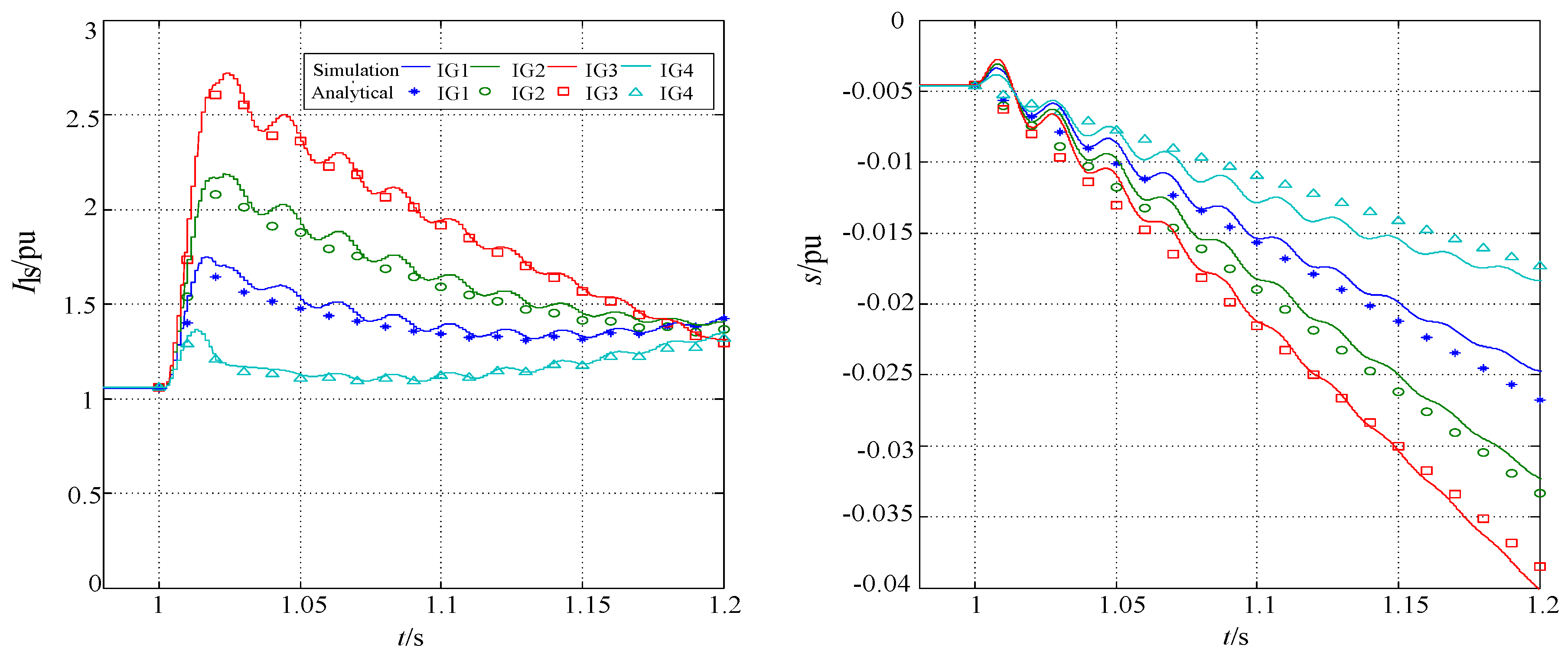
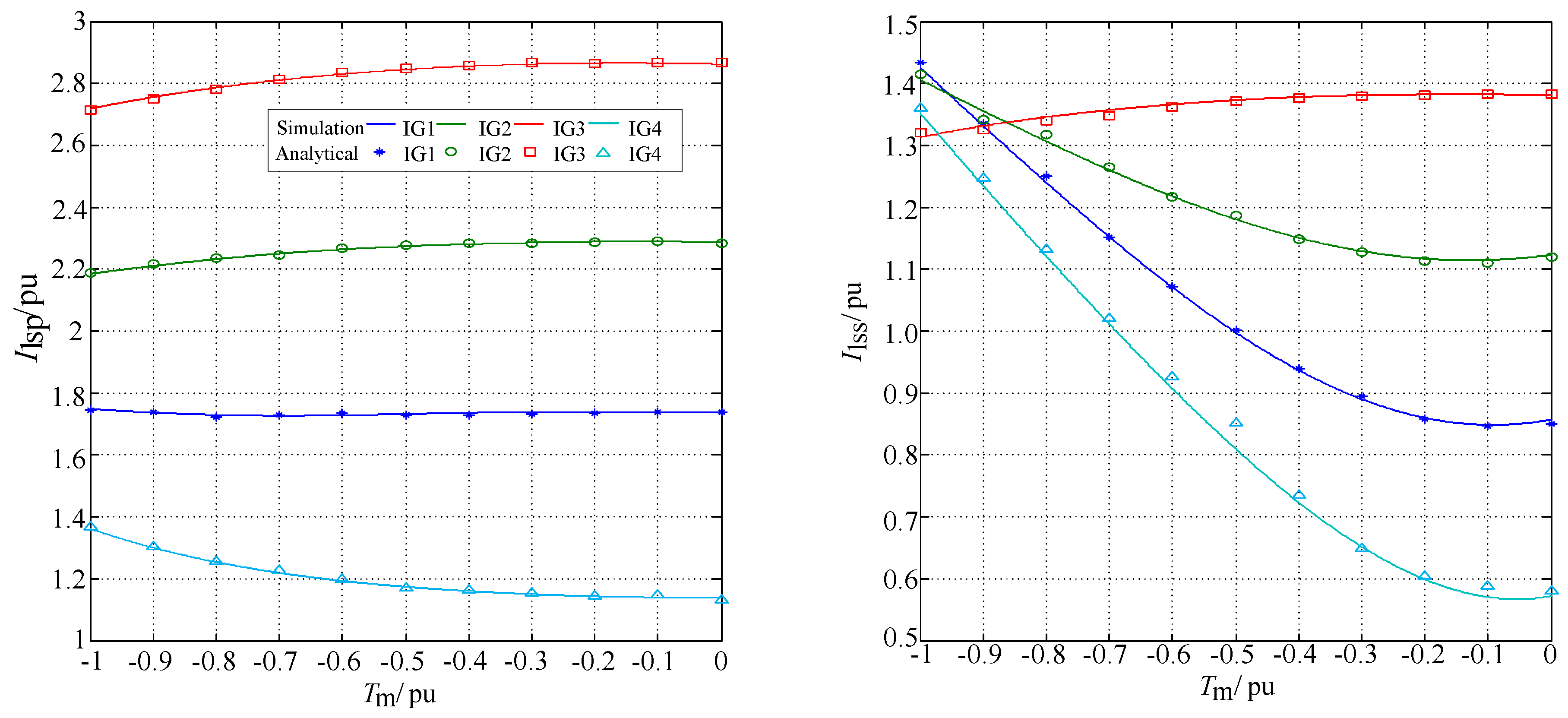
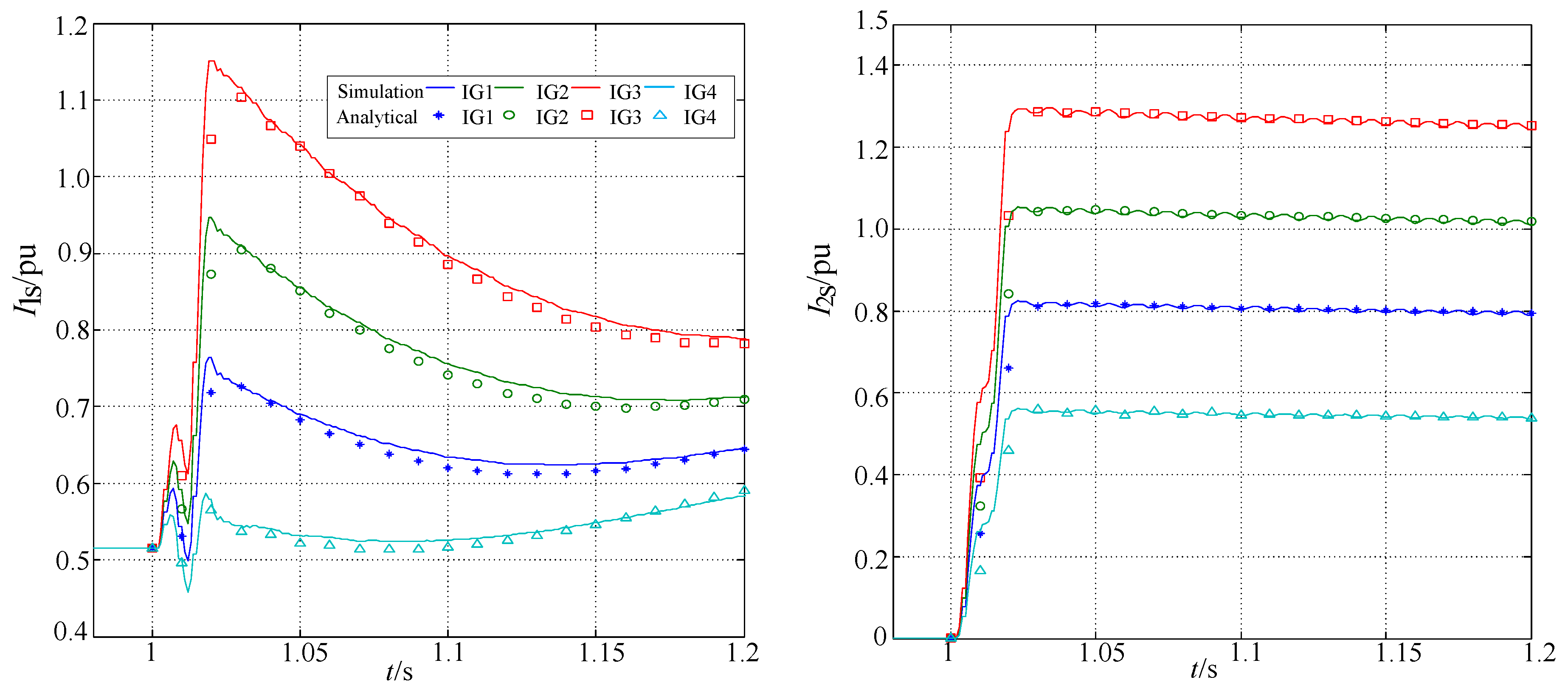
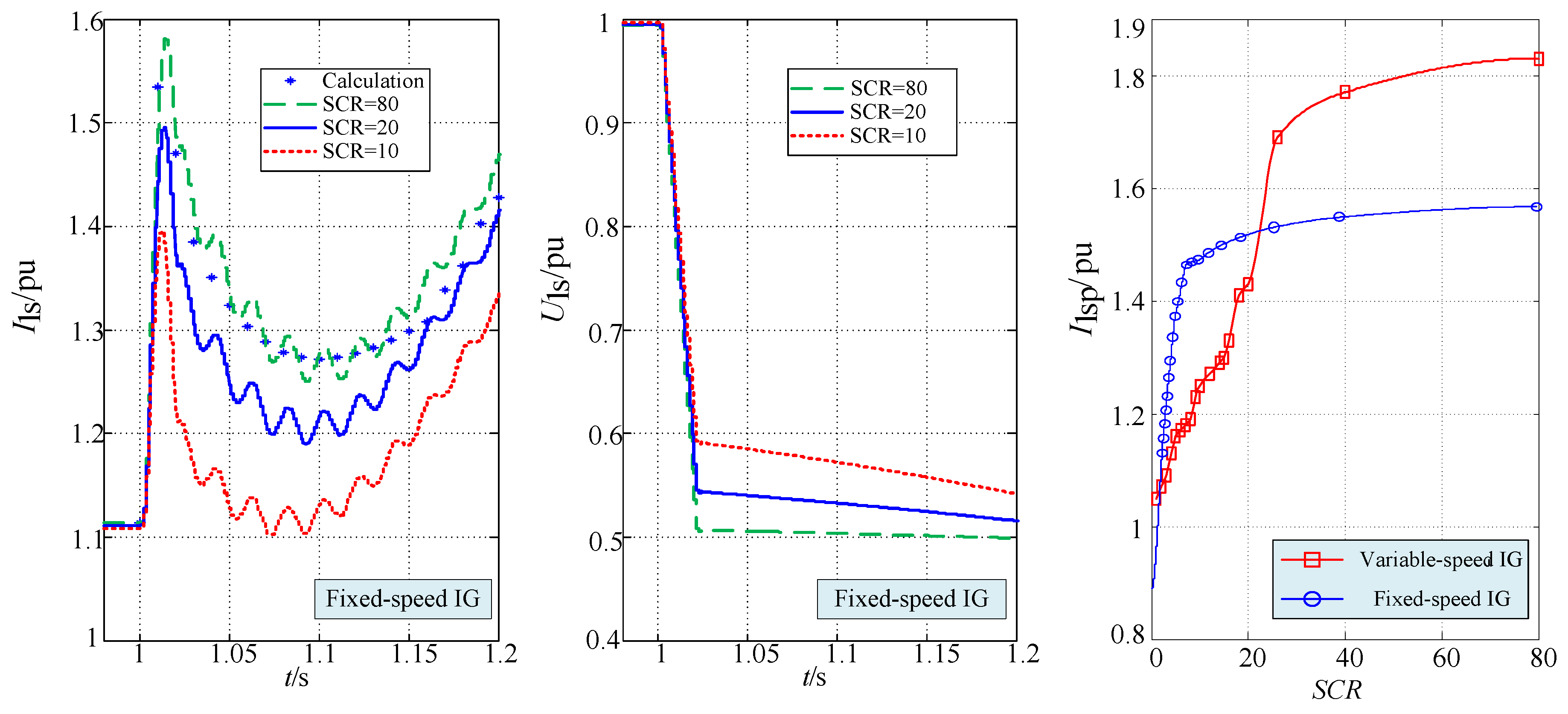
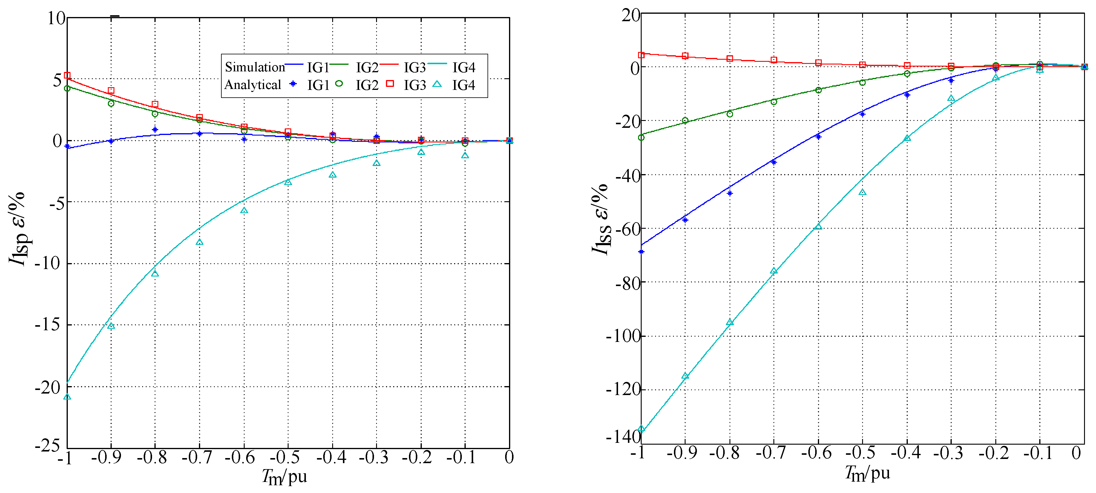
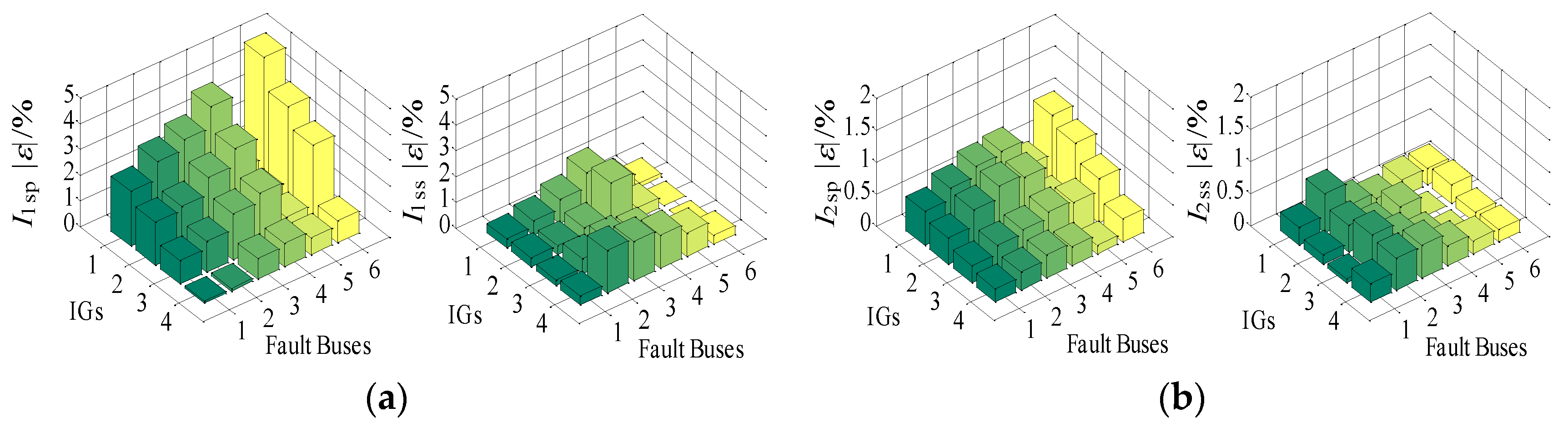
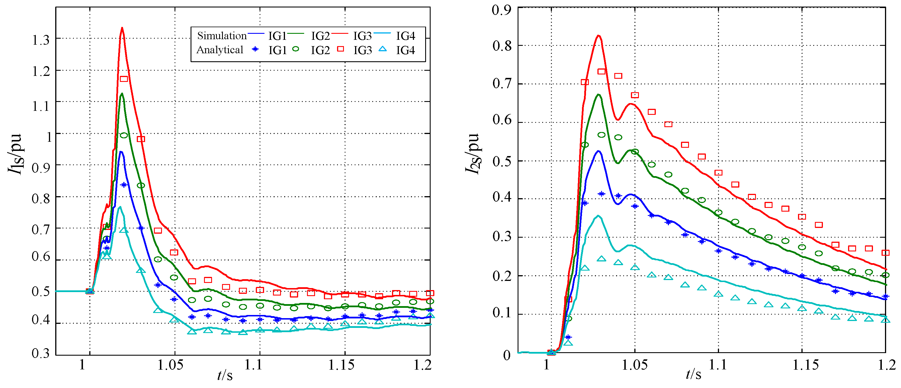
5.1. Three-Phase Short Circuit of Fixed-Speed IGs

When four IGs in Figure 10 are fixed-speed IGs, the short-circuit currents and slips of IG1 to IG4 when a three phase fault occurs at node 4 are shown in Figure 11, where the mechanical torques of IGs are T_m2 = T_m3 = T_m4 = −1.0. The short-circuit currents rise to the peak value after the fault that occurrs at t = 1.0s, and then transition to the steady state with the change of terminal voltages and slips. The simulation results are clearly accordant with the calculated results using the analytical method.

Figure 11 shows that the peak value I_1sp occurs at the second point of calculated results because I_1s is the RMS short-circuit current for a half cycle. The peak value I_1sp and steady-state value I_1ss can be given both by simulation and calculation, as shown in

Table 1. Short-circuit currents of fixed-speed IGs when three-phase short circuit occurs at bus 4.

	Induction Generators	IG1	IG2	IG3	IG4
	Analytical I1sp (pu)	1.642	2.079	2.605	1.317
I1sp	Simulation I1sp (pu)	1.745	2.187	2.716	1.369
	Relative error (%)	−5.90	−4.93	−4.09	−3.80
	Analytical I1ss (pu)	1.426	1.363	1.297	1.308
I1ss	Simulation I1ss (pu)	1.434	1.414	1.321	1.361
	Relative error (%)	−0.56	−3.61	−1.82	−3.89

, where the short-circuit current value of the 10th cycle is selected as the steady-state value. The proposed method has a relative error within ±6%. The voltages of IG3, IG2, IG1, and IG4 increase in turn while their currents decrease in turn because of the increasing electrical distance from IG to the fault node. Given that the voltage drop of IG4 at the adjacent feeder is the smallest, the peak value and steady-state value of IG4 are near each other.

Figure 12 shows the calculation and simulation results of the short-circuit current with the variable mechanical torque of one IG and a 0.1 change step under the assumption that the mechanical torques of the other three IGs remain unchanged. The simulated and calculated results with the proposed method are basically similar in the figure. The short-circuit currents calculated with zero mechanical torque are the same as the results with zero slips, which do not depend on the torque. The errors of the short-circuit currents with zero slips to the currents with different torques are shown in Figure 13. The relative errors of the peak and steady state value increase with the increase of −T_m.

Figure 13 shows that the larger the electrical distances from IG to the fault node, the more significant the rotor speed changes affect the short-circuit currents, and the smaller the peak and steady-state values calculated with zero slip. Even when taking the variation of terminal voltages is taken into account, the error of the short-circuit current may still exceed ±10% when constant speed sequence models are adopted in the iterative calculation. Such an effect may be due to the effect of slip variation on the positive sequence component of the short-circuit current. The errors of the peak value are mainly caused by different initial slips, whereas the errors of the steady-state value are decided by slip variations. Hence, the errors of steady-state values with zero slips are considerably bigger than the errors of peak values.

5.2. Two-Phase Short Circuit of Fixed-Speed IGs

The positive and negative sequence components of the short-circuit current of fixed-speed IGs with a phase B to phase C fault at node 6 are shown in Figure 14, where the mechanical torques of IGs are T_m1 = T_m2 = T_m3 = T_m4 = −0.5. The simulated and calculated results of the peak and steady-state value shown in

Table 2. Short-circuit currents of fixed-speed IGs when two-phase short-circuit occurs at bus 6.

	Induction Generators	IG1	IG2	IG3	IG4
	Analytical I1sp (pu)	0.727	0.911	1.116	0.582
I1sp	Simulation I1sp (pu)	0.765	0.947	1.151	0.587
	Relative error (%)	−4.97	−3.80	−3.04	−0.85
	Analytical I1ss (pu)	0.645	0.712	0.789	0.573
I1ss	Simulation I1ss (pu)	0.644	0.712	0.789	0.575
	Relative error (%)	0.16	0	0	−0.35
	Analytical I2sp (pu)	0.813	1.042	1.283	0.55
I2sp	Simulation I2sp (pu)	0.822	1.052	1.292	0.552
	Relative error (%)	−1.09	−0.95	−0.70	−0.36
	Analytical I2ss (pu)	0.790	1.012	1.244	0.537
I2ss	Simulation I2ss (pu)	0.793	1.021	1.248	0.538
	Relative error (%)	−0.38	−0.88	−0.32	−0.19

are almost same. Owing to the half-cycle lag of the real maximum value of I_1s has a half cycle lag compared with that of I_2s in the instantaneous current waveforms, the peak values of I_1s and I_2s are the third and second points in the calculation results respectively.

Similar with the three-phase short circuit, the difference between the steady-state and peak values of the positive and negative sequence components for IG4 is at the minimum with a two-phase fault occurring at node 6. The negative sequence components of short-circuit currents are determined only by the negative sequence terminal voltage, whereas the positive components of short-circuit currents depend upon the rotor flux attenuation associated with the slip and terminal voltage. Thus, the attenuation degrees of the negative sequence short-circuit currents of IG1, IG2, and IG3 are less than the degrees of their positive sequence components.

Figure 15 shows the relative errors of the proposed method with a two-phase fault at different nodes in the distribution network. With the slip variation, the coupling relation between terminal voltages, and the sequence networks during the fault considered, the absolute values of the relative errors for the steady-state value are observed to be less than the absolute value of the relative errors for the peak value. The relative errors of the proposed method for short-circuit calculation are within ±5%.

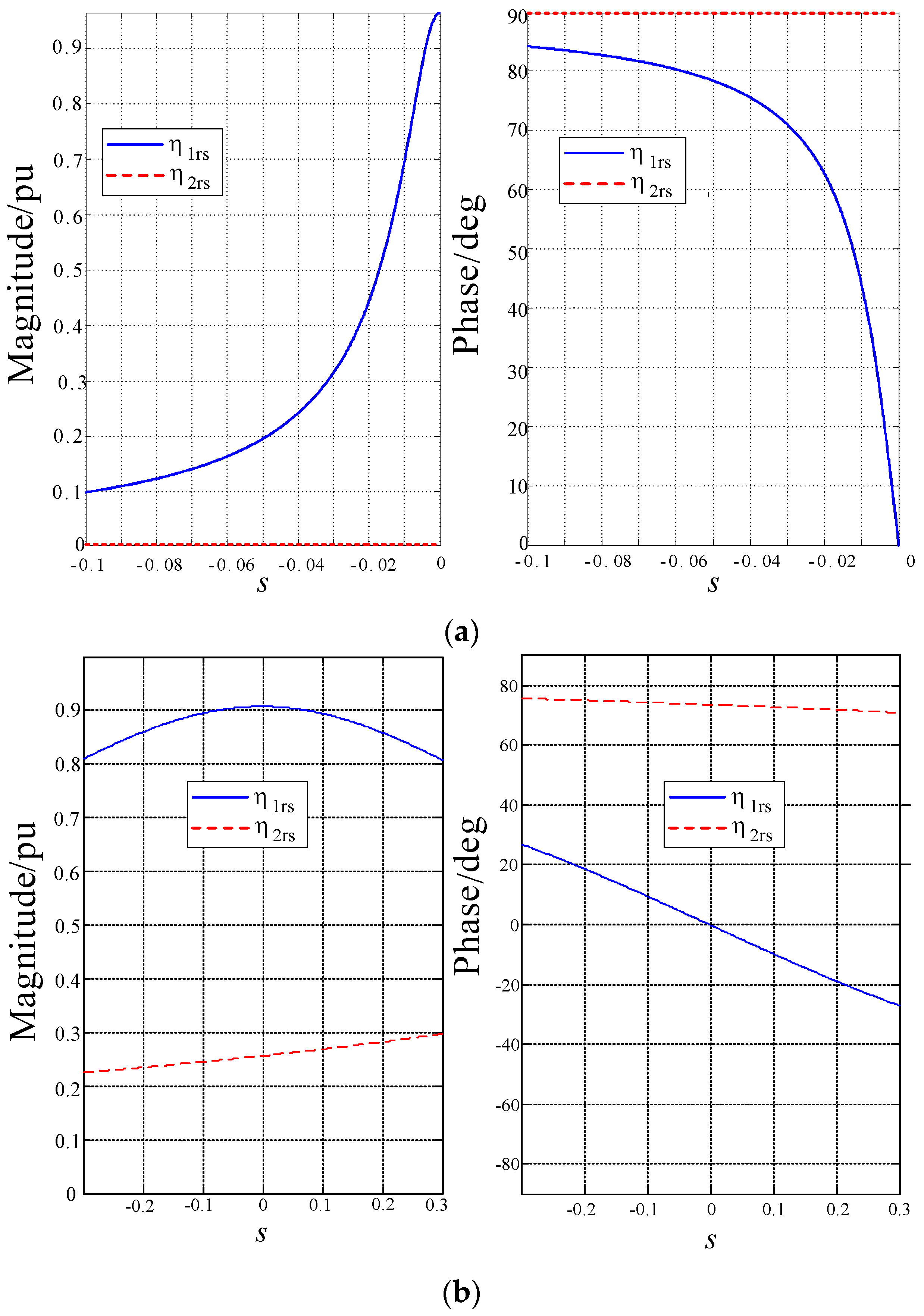
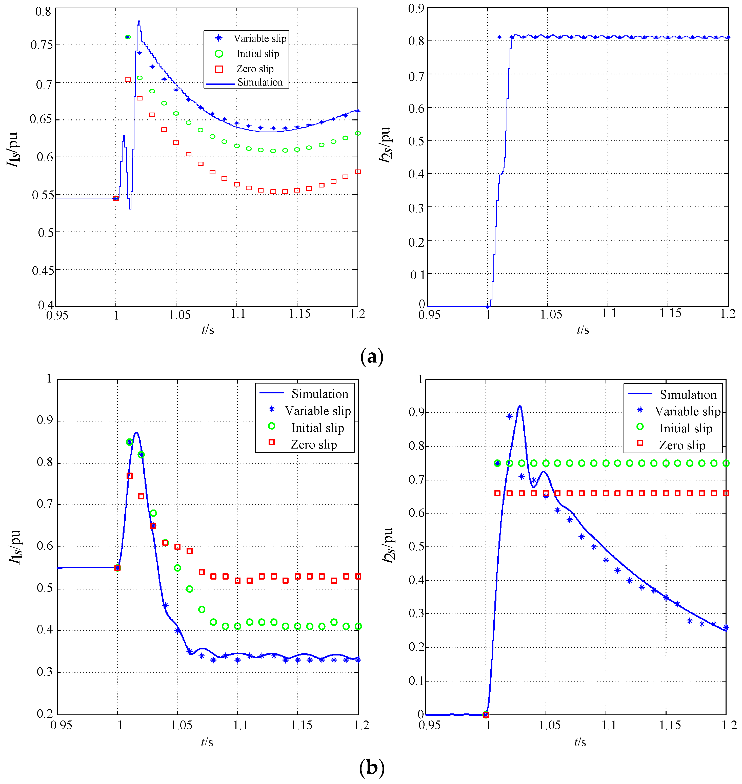
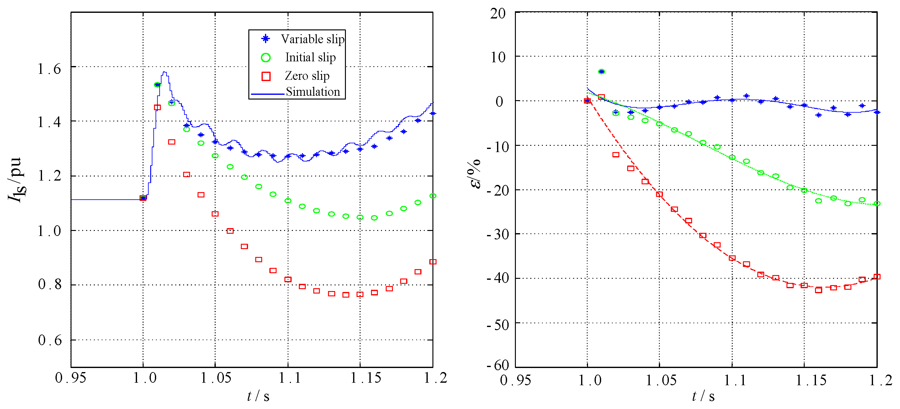
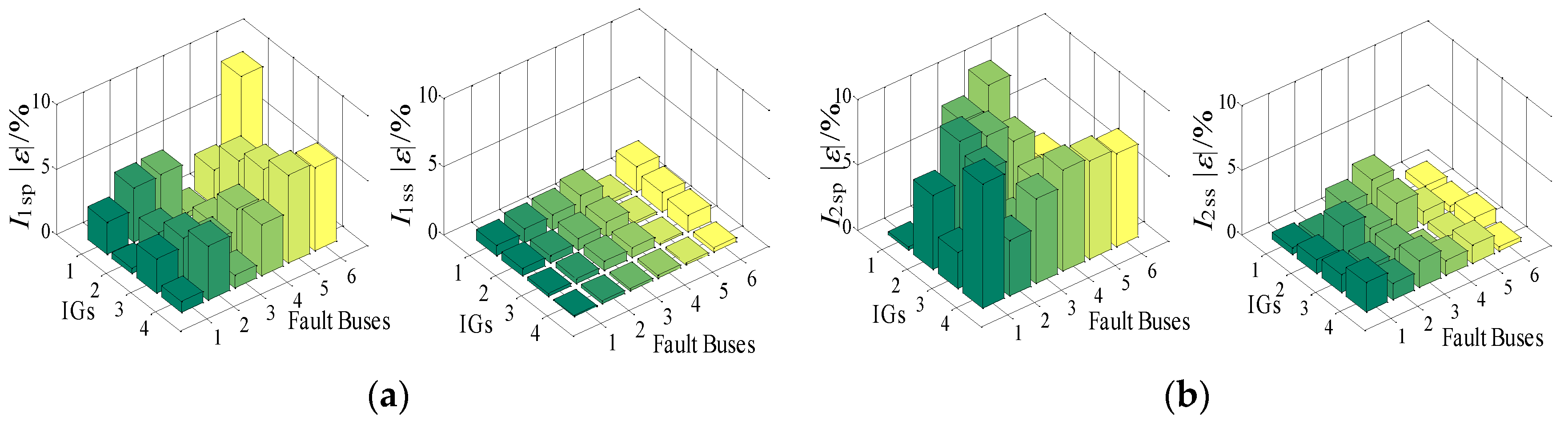
5.3. Two-Phase Short Circuit of Variable-Speed IGs

Figure 16 shows the positive and negative sequence components of the short-circuit current of variable-speed IGs with a phase B to phase C fault at node 6 when four IGs in the test system are variable-speed IGs. The short-circuit currents of the four variable-speed IGs decay rapidly after rising to the peak value, and the descent rate of the negative components are slower than that of the positive components. The calculated results of the short-circuit currents by the analytical method are basically consistent with the dynamic simulation results in

Table 3. Short circuit currents of variable-speed IGs when two-phase short circuit occurs at bus 6.

	Induction Generators	IG1	IG2	IG3	IG4
	Analytical I1sp (pu)	0.856	1.093	1.196	0.715
I1sp	Simulation I1sp (pu)	0.937	1.104	1.308	0.765
	Relative error (%)	−8.62	−1.03	−0.81	−6.53
	Analytical I1ss (pu)	0.418	0.444	0.489	0.395
I1ss	Simulation I1ss (pu)	0.412	0.439	0.485	0.396
	Relative error (%)	1.37	1.09	0.86	−0.21
	Analytical I2sp (pu)	0.436	0.596	0.746	0.278
I2sp	Simulation I2sp (pu)	0.456	0.634	0.806	0.307
	Relative error (%)	−4.39	−5.99	−7.44	−9.45
	Analytical I2ss (pu)	0.159	0.185	0.219	0.102
I2ss	Simulation I2ss (pu)	0.158	0.183	0.208	0.103
	Relative error (%)	0.36	1.22	5.29	−0.65

.

The relative errors of the proposed method for variable-speed IGs are shown in Figure 17. The interactive process of the short-circuit current of variable-speed IGs with the distribution network is simplified by ignoring the delaying influence of the crowbar activation and the dynamic responses of the converter and its controller, factors that lead to relatively large calculation errors of the variable-speed IGs. According to the test results of variable-speed IGs, the maximum relative error of the method ranges from 10% to 15%.

6. Conclusions

This paper proposes an improved analytical method to calculate the sequence components of the short-circuit currents of multi-IG systems. The short-circuit calculation problem is formulated based on the transient response, slip variation of fixed-speed and variable-speed IGs, and parameters of distribution network, and is solved using the iteration technique. The results show that the coupling relationship among the short-circuit currents, slip variations and terminal voltages should be considered for the short-circuit calculation of IGs when the SCR is small. The proposed method is verified using dynamic simulation. Comparisons show that the analytical results are very close to the simulation results. Therefore, the proposed technique is an effective tool to determine the short-circuit currents of multi fixed-speed and variable-speed IGs, which are very useful for the fault analysis and protection of distribution networks. However, the simulation software requires additional computational burden and time to find the short-circuit currents. The analytical method can likewise provide more information to better understand the transient responses of IGs during grid faults and the related effects of IG and network parameters. Accordingly, an improved protection system for the distribution network can be designed.

References

1. Nimpitiwan, N.; Heydt, G.T.; Ayyanar, R.; Suryanarayana, S. Fault current contribution from synchronousmachine and inverter based distributed generators. IEEE Trans. Power Deliv. 2007, 22, 634–641. [Google Scholar] [CrossRef]
2. Akhmatov, V. Induction Generators for Wind Power; Multi Science: Essex, UK, 2007. [Google Scholar]
3. Freitas, W.; Vieira, J.C.M.; Morelato, A.; da Silva, L.C.P.; da Costa, V.F.; Lemos, F.A.B. Comparative analysis between synchronous and induction machines for distributed generation applications. IEEE Trans. Power Syst. 2006, 21, 301–311. [Google Scholar] [CrossRef]
4. Huening, W.C. Calculating short-circuit currents with contributions from induction motors. IEEE Trans. Ind. Appl. 1982, IA-18, 85–92. [Google Scholar] [CrossRef]
5. Morren, J.; de Haan, S.W.H. Short-circuit current of wind turbines with doubly fed induction generator. IEEE Trans. Energy Convers. 1991, 22, 174–180. [Google Scholar] [CrossRef]
6. Boutsika, T.N.; Papathanassiou, S.A. Short-circuit calculations in networks with distributed generation. Electr. Power Syst. Res. 2008, 78, 1181–1191. [Google Scholar] [CrossRef]
7. Sulawa, T.; Zabar, Z.; Czarkowski, D.; TenAmi, Y.; Birenbaum, L.; Lee, S. Evaluation of a 3-ϕ bolted short-circuit on distribution networks having induction generators at customer sites. IEEE Trans. Power Deliv. 2007, 22, 1965–1971. [Google Scholar] [CrossRef]
8. Trudnowski, D.J.; Gentile, A.; Khan, J.M.; Petritz, E.M. Fixed speed wind-generator and wind-park modeling for transient stability studies. IEEE Trans. Power Syst. 2004, 19, 1911–1917. [Google Scholar] [CrossRef]
9. Causebrook, A.; Atkinson, D.J.; Jack, A.G. Fault ride-through of large wind farms using series dynamic braking resistors. IEEE Trans. Power Syst. 2007, 22, 966–975. [Google Scholar] [CrossRef]
10. Pannell, G.; Atkinson, D.J.; Zahawi, B. Analytical study of grid-fault response of wind turbine doubly fed induction generator. IEEE Trans. Energy Convers. 2010, 25, 1081–1091. [Google Scholar] [CrossRef]
11. Ouhrouche, M. Transient analysis of a grid connected wind driven induction generator using a real-time simulation platform. Renew. Energy 2009, 34, 801–806. [Google Scholar] [CrossRef]
12. Vicatos, M.S.; Tegopoulos, J.A. Transient state analysis of a doubly-fed induction generator under three phase short circuit. IEEE Trans. Energy Convers. 1991, 6, 62–68. [Google Scholar] [CrossRef]
13. Lopez, J.; Gubia, E.; Sanchis, P.; Roboam, X.; Marroyo, L. Wind turbines based on doubly fed induction generator under asymmetrical voltage dips. IEEE Trans. Energy Convers. 2008, 23, 321–330. [Google Scholar] [CrossRef]
14. Sulla, F.; Svensson, J.; Samuelsson, O. Symmetrical and unsymmetrical short-circuit current of squirrel-cage and doubly-fed induction generators. Electr. Power Syst. Res. 2011, 81, 1610–1618. [Google Scholar] [CrossRef]
15. Mohseni, M.; Islam, S.M.; Masoum, M.A.S. Impacts of symmetrical and asymmetrical voltage sags on DFIG-based wind turbines considering phase-angle jump, voltage recovery, and sag parameters. IEEE Trans. Power Electron. 2011, 26, 1587–1598. [Google Scholar] [CrossRef]
16. Howard, D.F.; Habetler, T.G.; Harley, R.G. Improved sequence network model of wind turbine generators for short-circuit studies. IEEE Trans. Energy Convers. 2012, 27, 968–977. [Google Scholar] [CrossRef]
17. Anderson, P.M. Analysis of Faulted Power Systems; Institute of Electrical and Electronics Engineers (IEEE): Piscataway, NJ, USA, 1995. [Google Scholar]
18. Li, H.; Zhao, B.; Yang, C.; Chen, H.W.; Chen, Z. Analysis and estimation of transient stability for a grid-connected wind turbine with induction generator. Renew. Energy 2011, 36, 1469–1476. [Google Scholar] [CrossRef]
19. El-Naggar, A.; Erlich, I. Analysis of fault current contribution of doubly-fed induction generator wind turbines under unbalanced grid faults. Renew. Energy 2016, 91, 137–146. [Google Scholar] [CrossRef]
20. Grilo, A.P.; Mota, A.A.; Mota, L.T.; Freitas, W. An analytical method for analysis of large-disturbance stability of induction generators. IEEE Trans. Power Syst. 2007, 22, 1861–1869. [Google Scholar] [CrossRef]
21. Sun, T.; Chen, Z.; Blaabjerg, F. Flicker study on variable speed wind turbines with doubly fed induction generators. IEEE Trans. Energy Convers. 2005, 20, 896–905. [Google Scholar] [CrossRef]
22. Rodriguez, P.; Timbus, A.V.; Teodorescu, R.; Liserre, M.; Blaabjerg, F. Flexible active power control of distributed power generation systems during grid faults. IEEE Trans. Ind. Electron. 2007, 54, 2583–2592. [Google Scholar] [CrossRef]
Figure 1. Positive and negative sequence steady-state equivalent circuits of an IG: (a) Positive sequence circuit, (b) Negative sequence circuit.
Energies 09 00277 g001
Figure 2. Positive and negative sequencecorrelation coefficients between stator and rotor flux: (a) a fixed-speed IG, (b) a variable-speed IG.
Energies 09 00277 g002
Figure 3. An equivalent circuit for stator flux DC component in the rotor reference frame.
Energies 09 00277 g003
Figure 4. DC component correlation coefficient between stator and rotor flux.
Energies 09 00277 g004
Figure 5. Positive and negative sequence correlation coefficients between stator and rotor flux of a fixed-speed IG.
Energies 09 00277 g005
Figure 6. Two-phase short-circuit current with and without rotor slip change: (a) a fixed-speed IG, (b) a variable-speed IG.
Energies 09 00277 g006
Figure 7. Short-circuit current and terminal voltage of IGs with different penetration levels.
Energies 09 00277 g007
Figure 8. Schematic diagram of coupling relation between short-circuit current of IGs and distribution network.
Energies 09 00277 g008
Figure 9. Composite sequence network of two-phase short-circuit with negative sequence voltage.
Energies 09 00277 g009
Figure 10. Four-IG test system.
Energies 09 00277 g010
Figure 11. Short-circuit currents and rotor slips of fixed-speed IGs when three-phase short-circuit occurs at bus 4.
Energies 09 00277 g011
Figure 12. Three-phase short-circuit current of fixed-speed IGs when the torque is varying.
Energies 09 00277 g012
Figure 13. Relative errors of three-phase short-circuit currents of fixed-speed IGs with zero slips.
Energies 09 00277 g013
Figure 14. Short-circuit current sequence components of fixed-speed IGs when two-phase short circuit occurs at bus 6.
Energies 09 00277 g014
Figure 15. Relative errors of short-circuit currents of fixed-speed IGs when two-phase short circuit occurs: (a) Positive sequence component, (b) Negative sequence component.
Energies 09 00277 g015
Figure 16. Short-circuit current sequence components of variable-speed IGs when two-phase short circuit occurs at bus 6.
Energies 09 00277 g016
Figure 17. Relative errors of short-circuit currents of variable-speed IGs when two-phase short circuit occurs: (a) Positive sequence component, (b) Negative sequence component.
Energies 09 00277 g017