
A Novel DC-Bus Sensor-less MPPT Technique for Single-Stage PV Grid-Connected Inverters


 ,
,  ,
,  and
and
Abstract
:1. Introduction
2. Derivation of the Proposed Technique
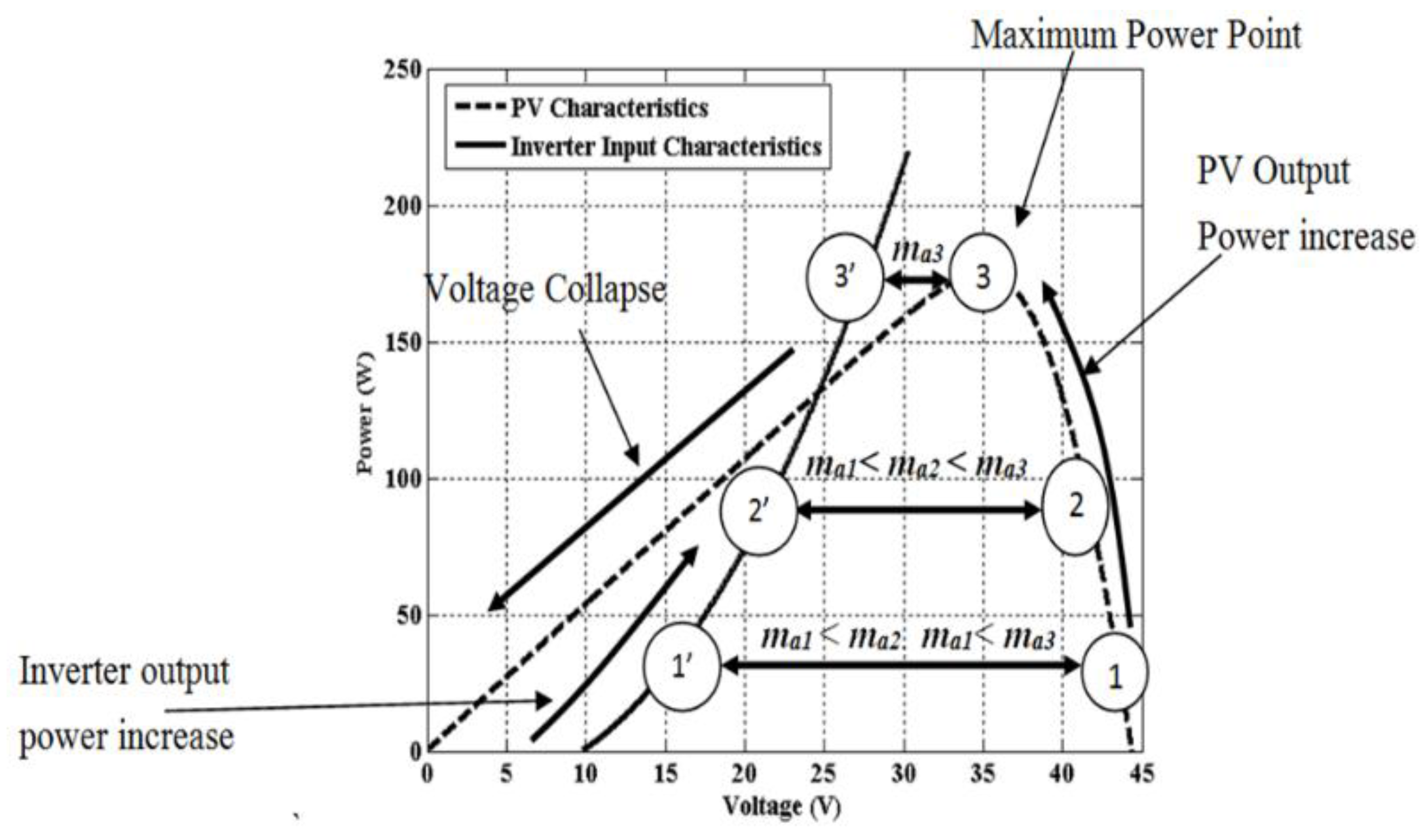
2.1. Typical Single-Stage Configuration Response
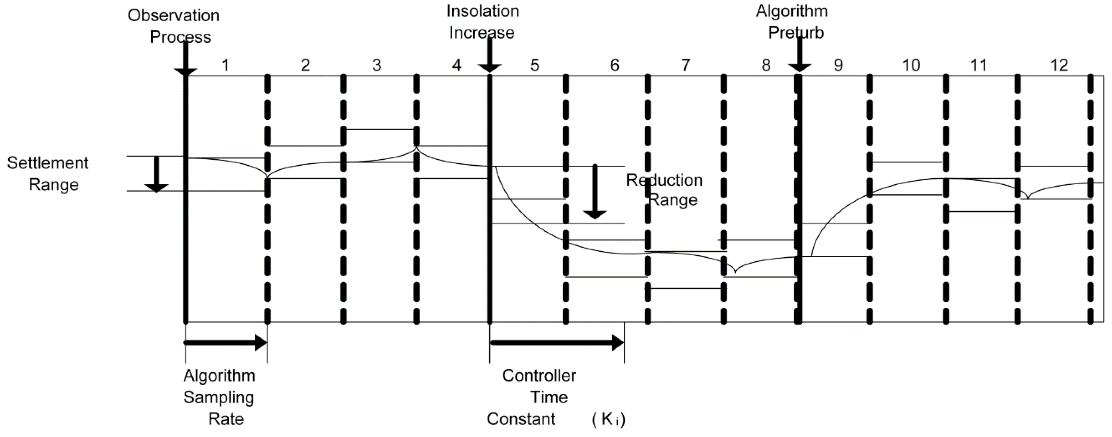
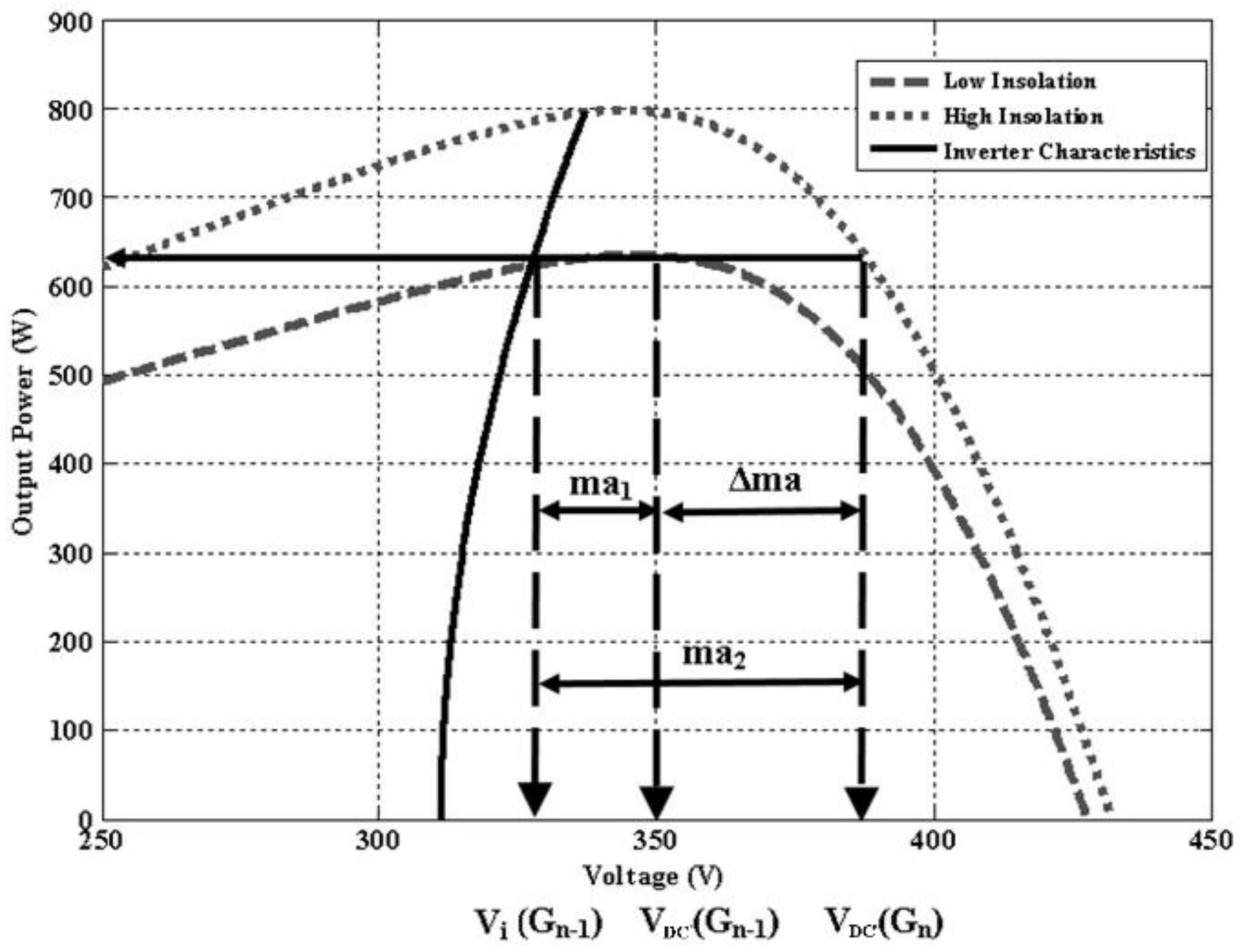
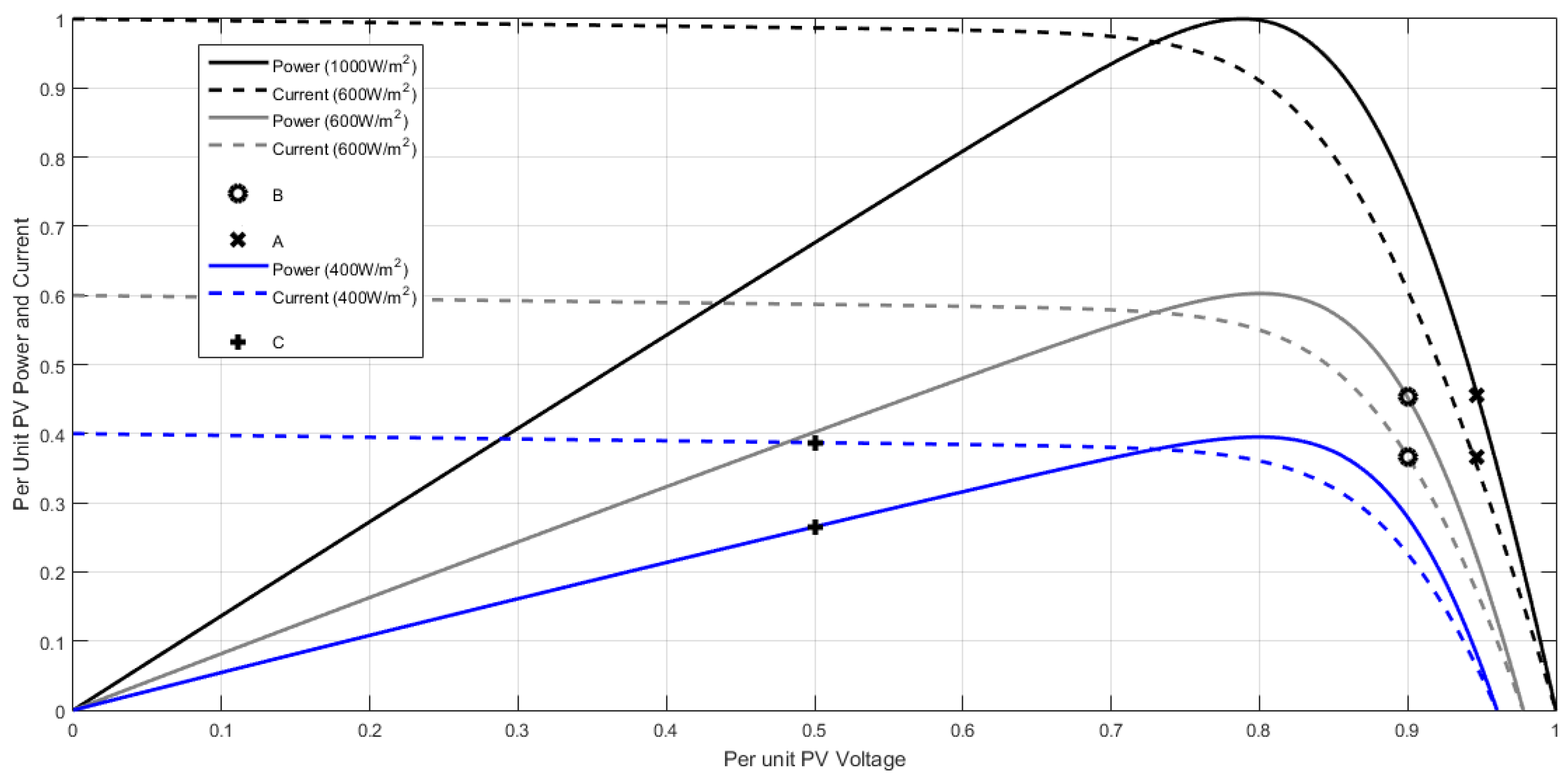
2.2. Effect of Change in Insolation
- Step increase in insolation while operating at or below the previous maximum power point;
- Step decrease in insolation while operating below the new maximum power point;
- Step decrease in insolation while operating above the new maximum power point.
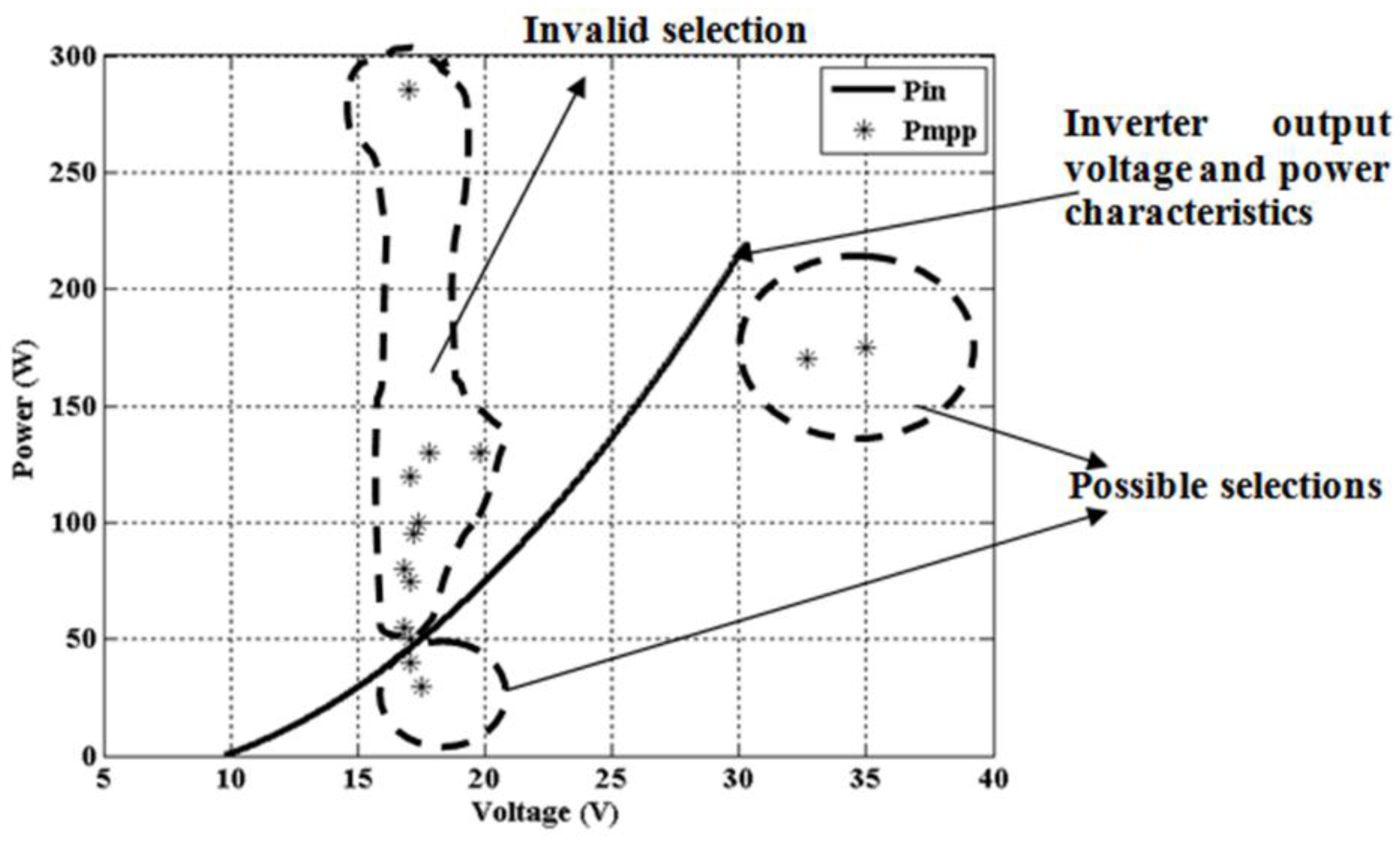
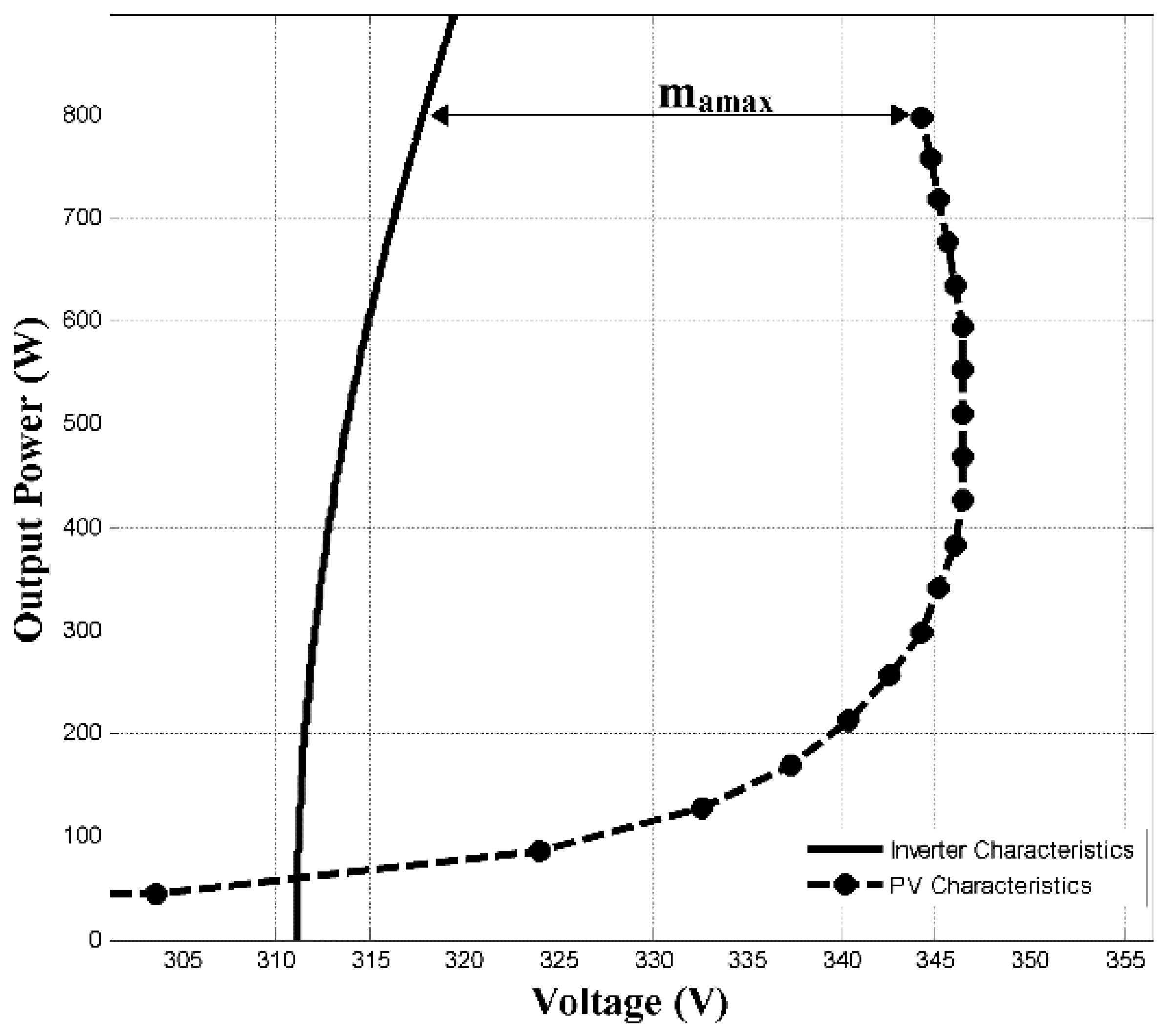
2.3. PV Selection Limits
- Continue operation at a power point below the maximum power as long as the inverter and PV voltage criteria are satisfied.
- Set a cut-off power for the inverter such that the inverter will cease operation at very low power values.
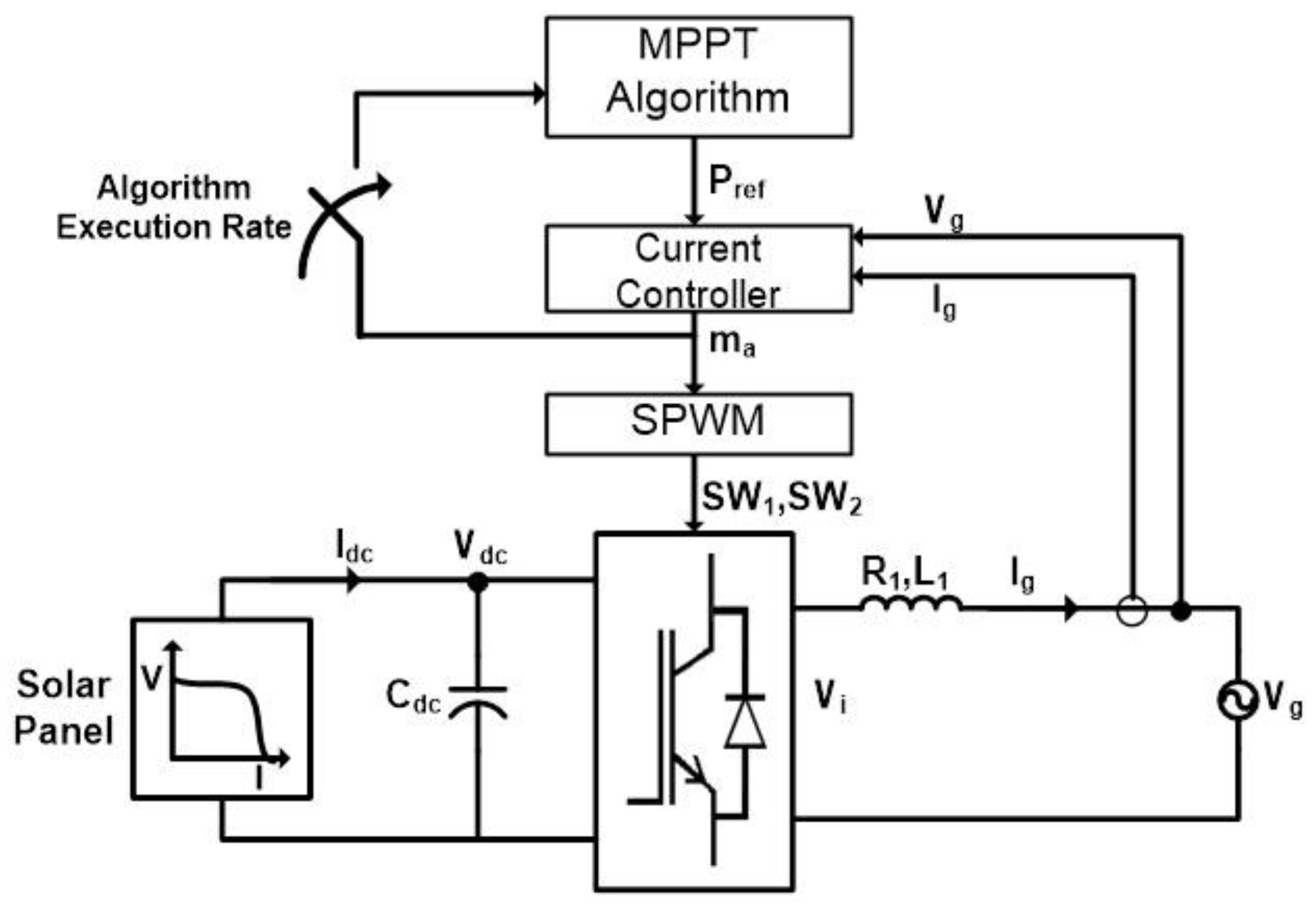
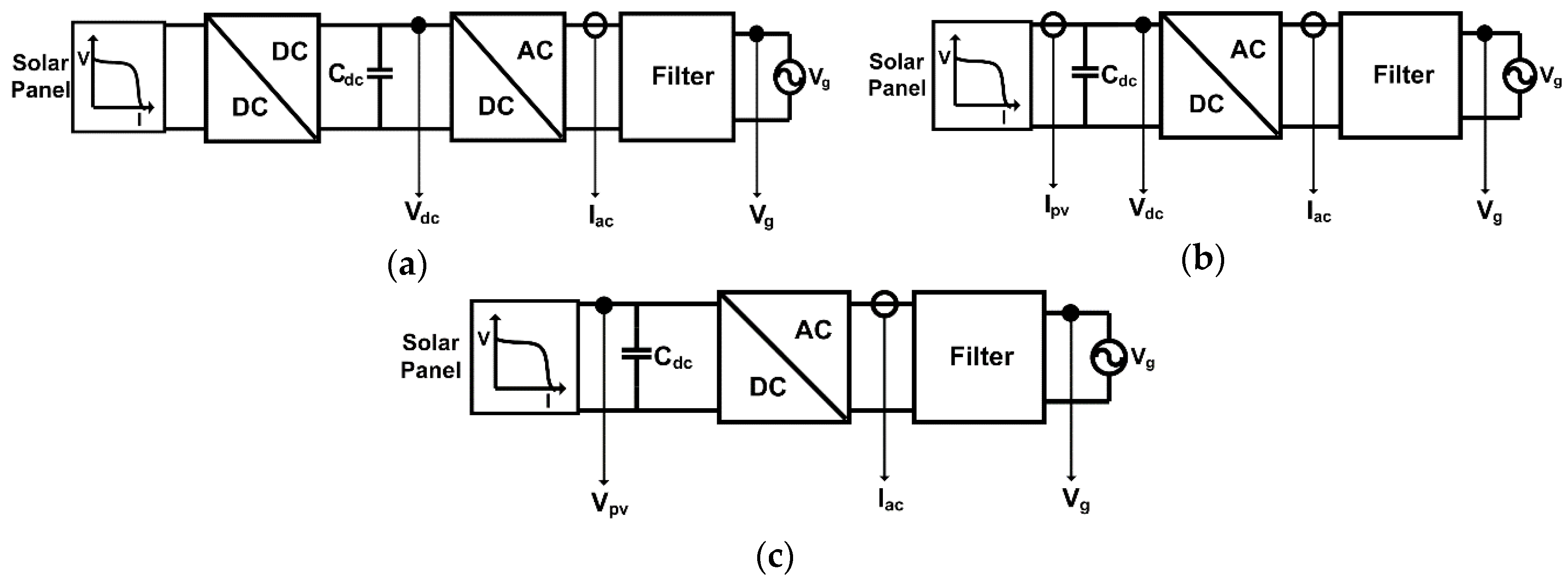
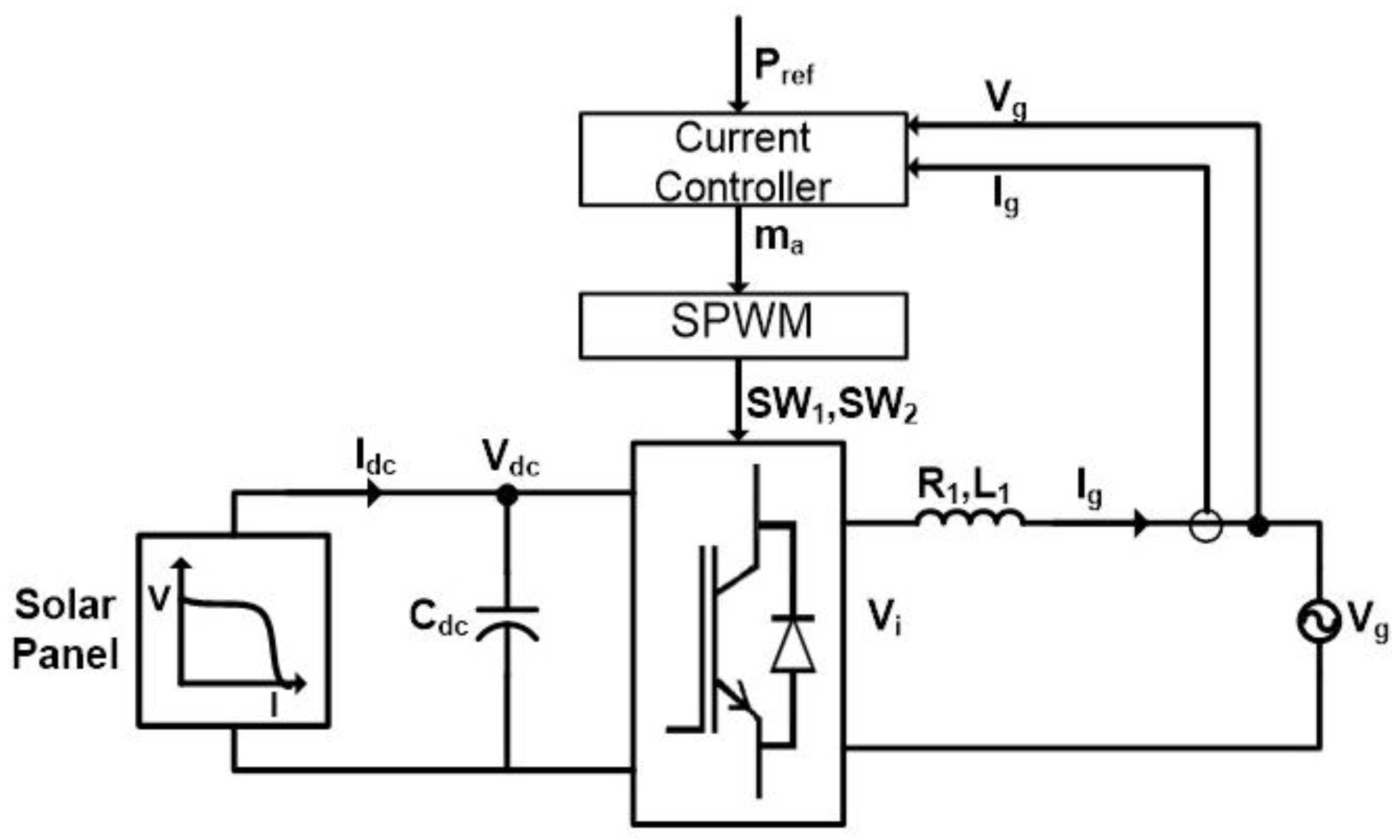
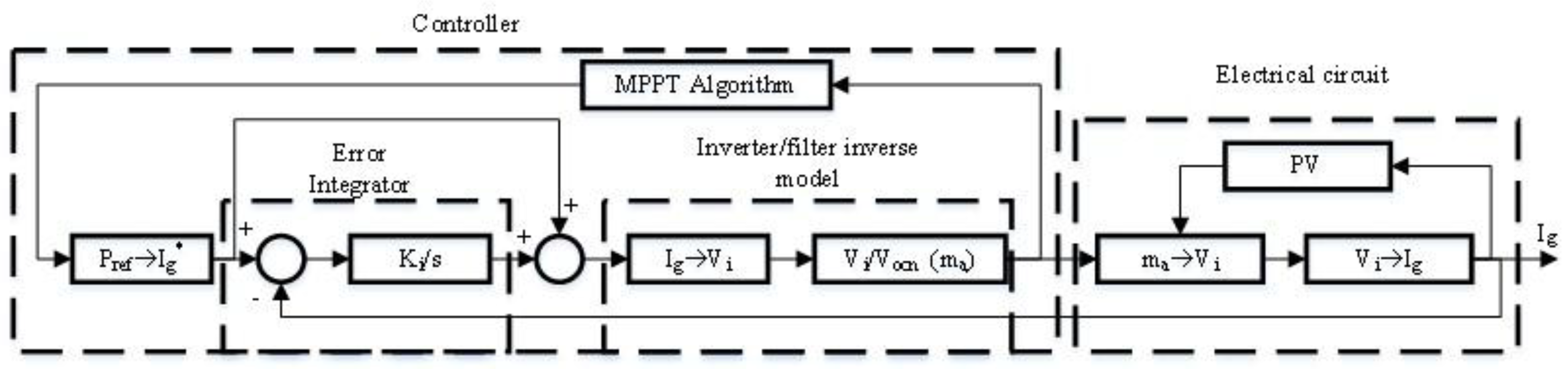
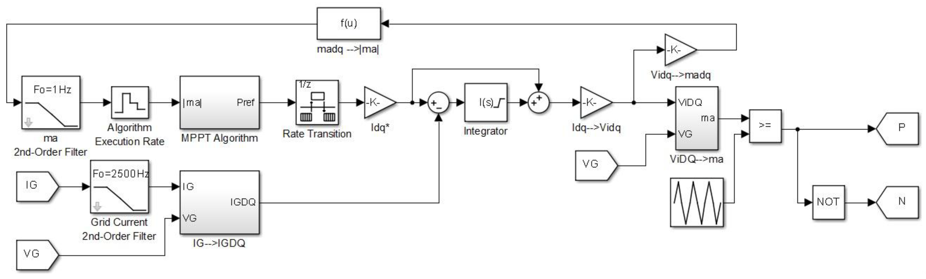
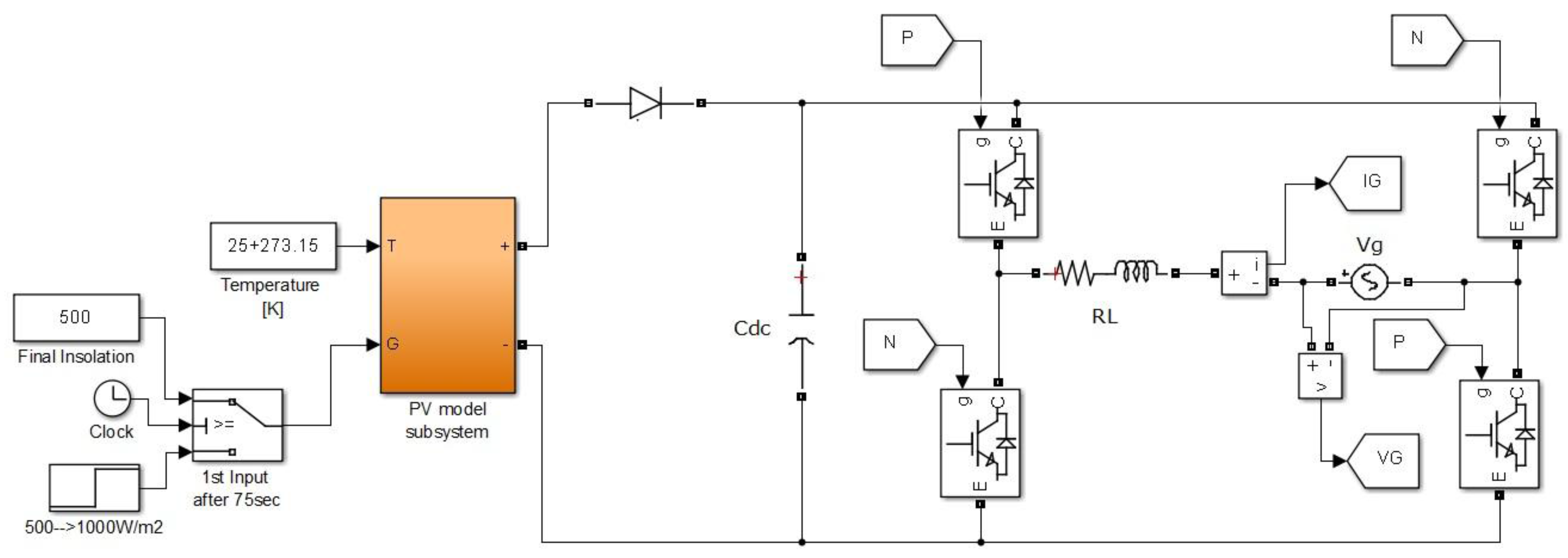
3. Proposed System
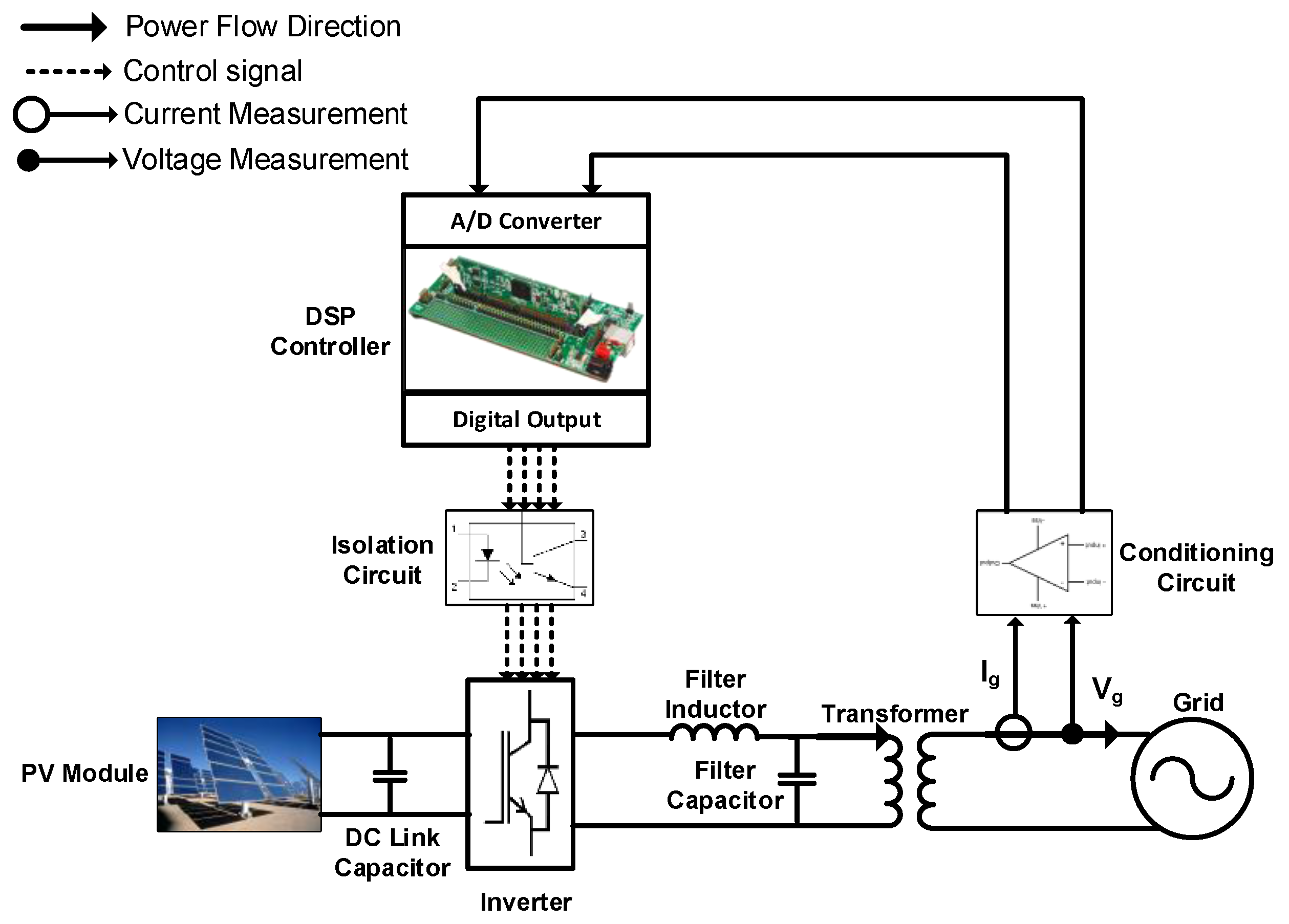
3.1. Configuration
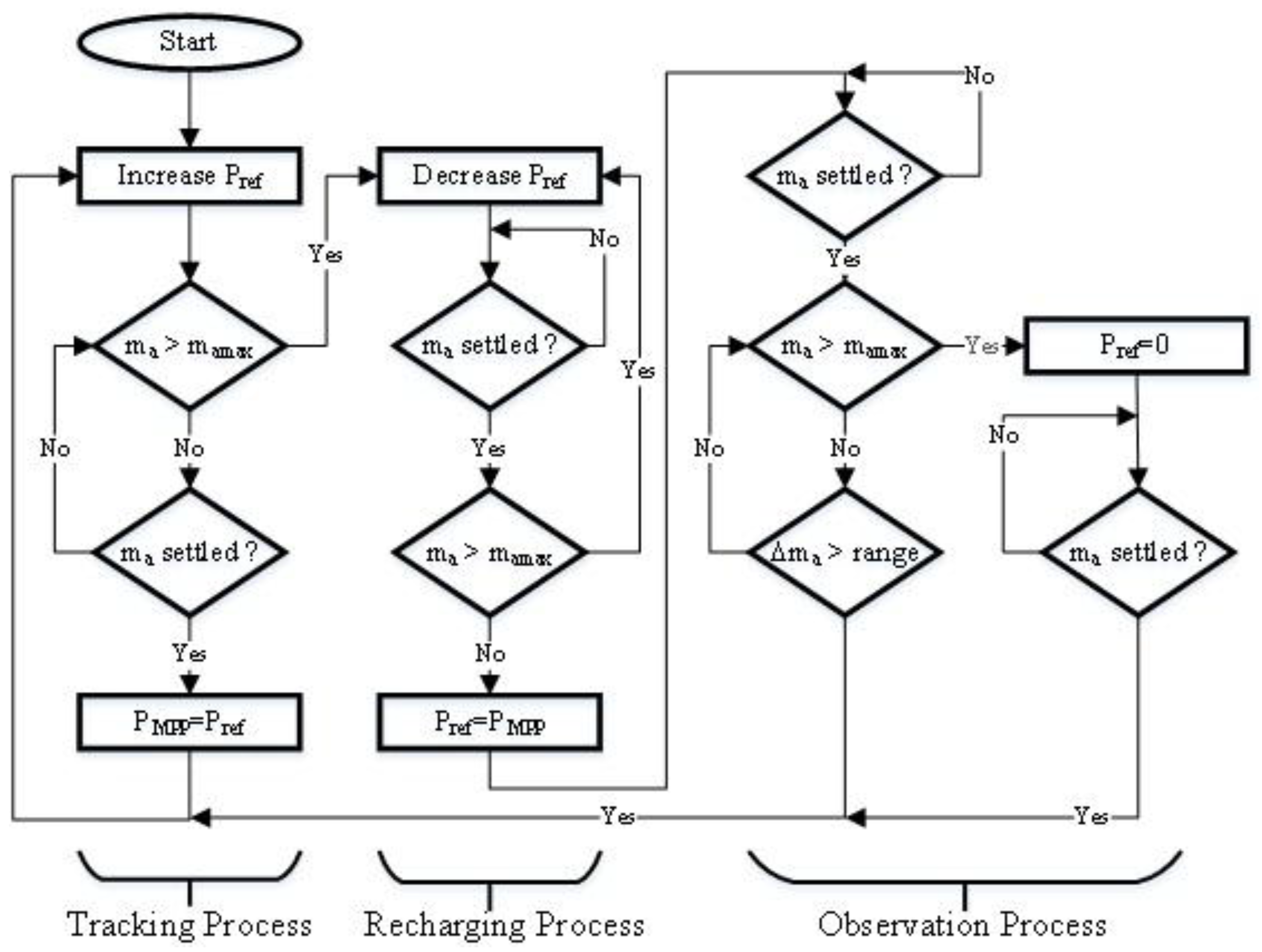
3.2. Algorithm
3.2.1. Tracking Process
3.2.2. Recharging Process
3.2.3. Observation Process
3.3. Controller
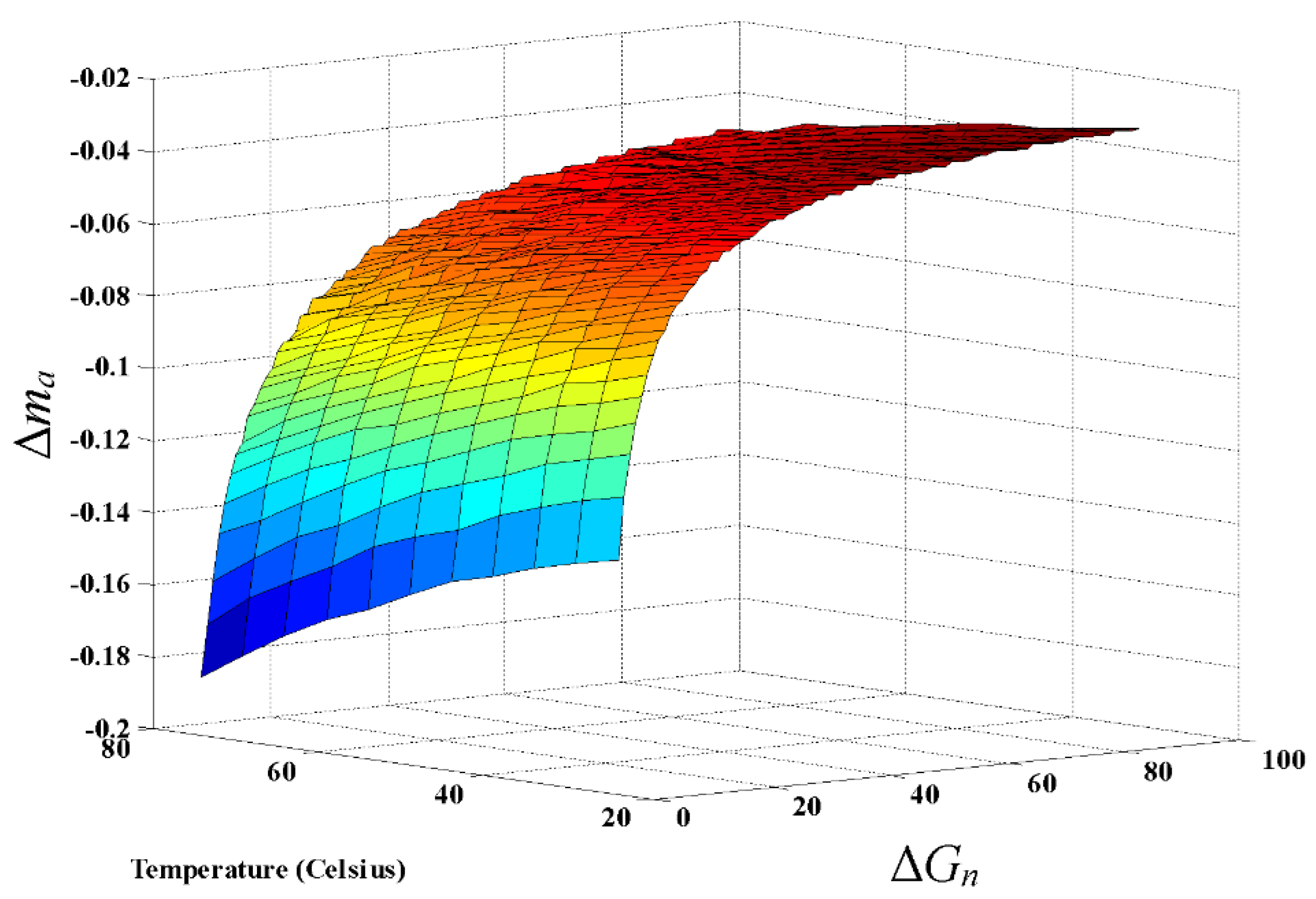
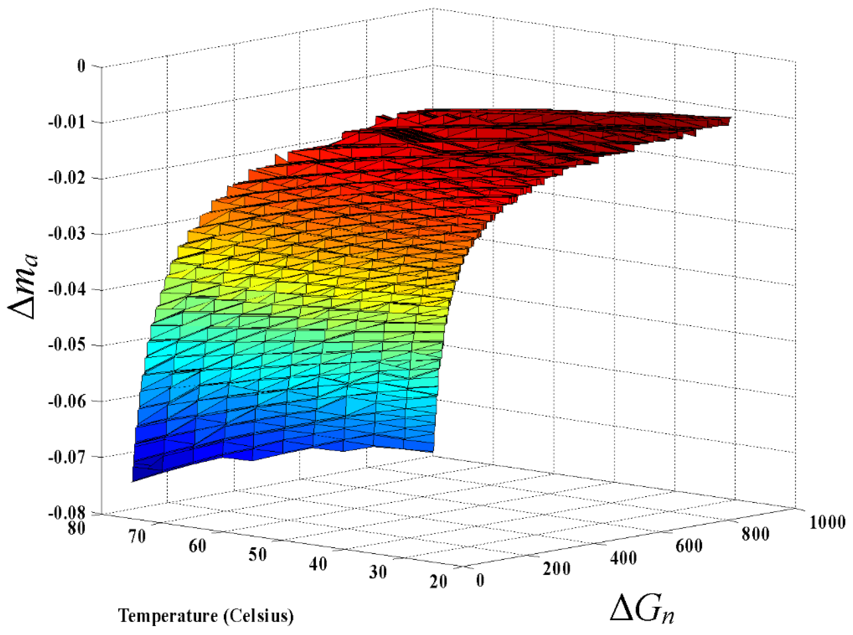
3.4. Parameters
- Choosing a suitable ΔG: this is a design selection based on the required sensing of changes in insolation. Decreasing the value of ΔG leads to an increased accuracy of obtaining true maximum power.
- Find Vdc(Gn−1) and Pout(Gn−1): using PV model in Equation (5), calculate the PV maximum output power at nominal temperature and insolation below maximum by ΔG.
- Find Vdc(Gn): calculate the PV voltage at maximum insolation that would give the same output power at the lower insolation calculated earlier:
4. Simulation Results
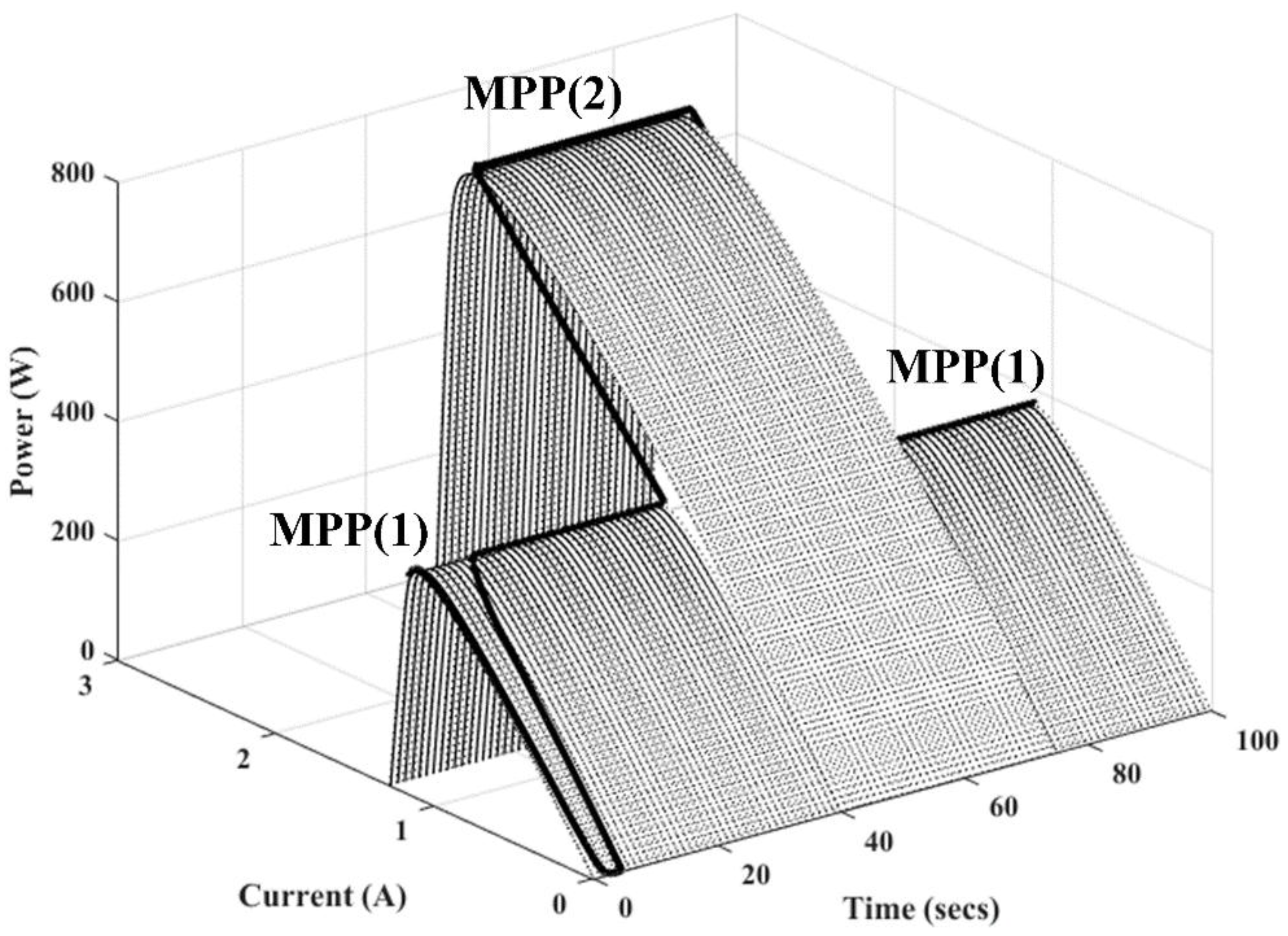
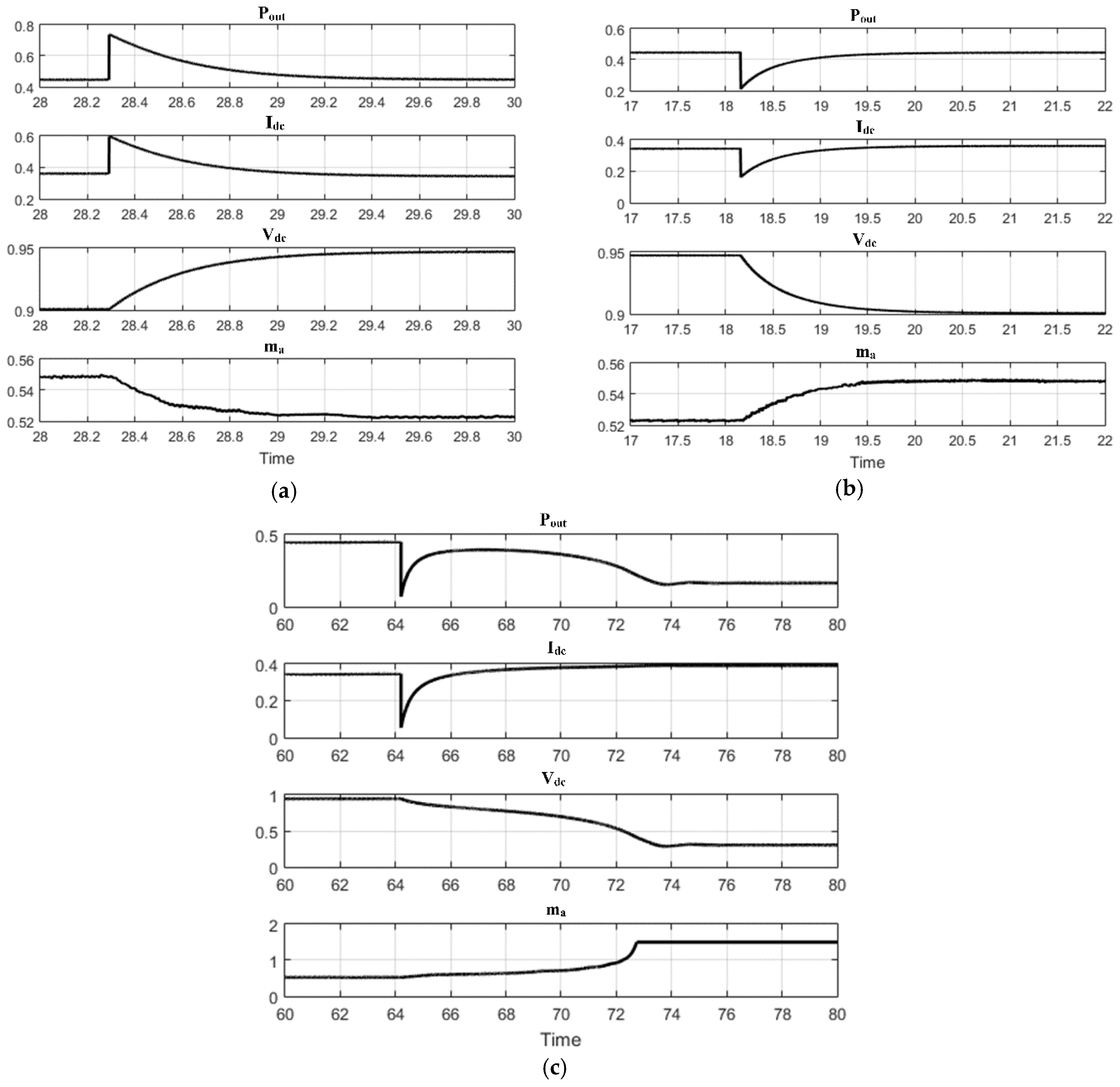
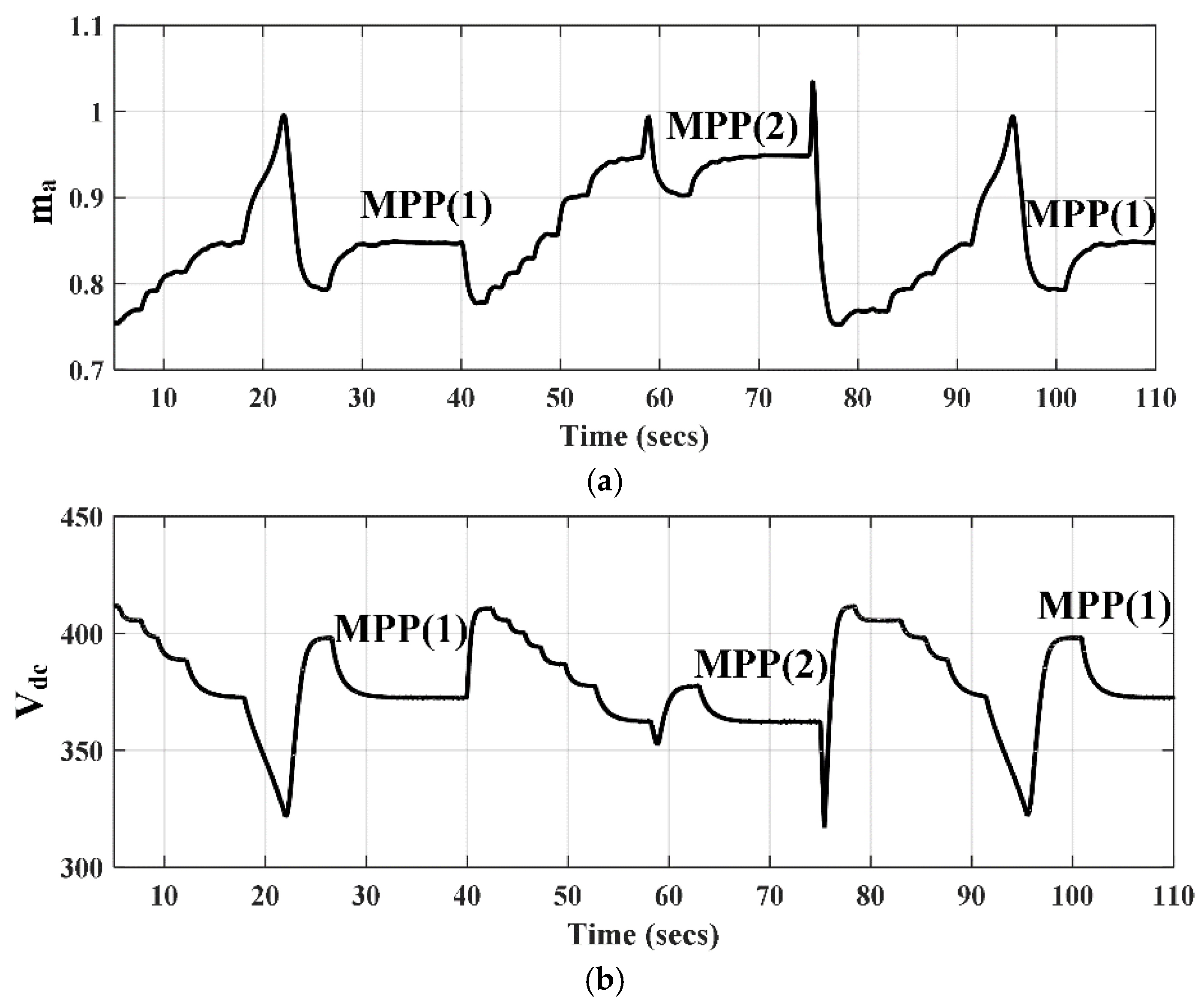
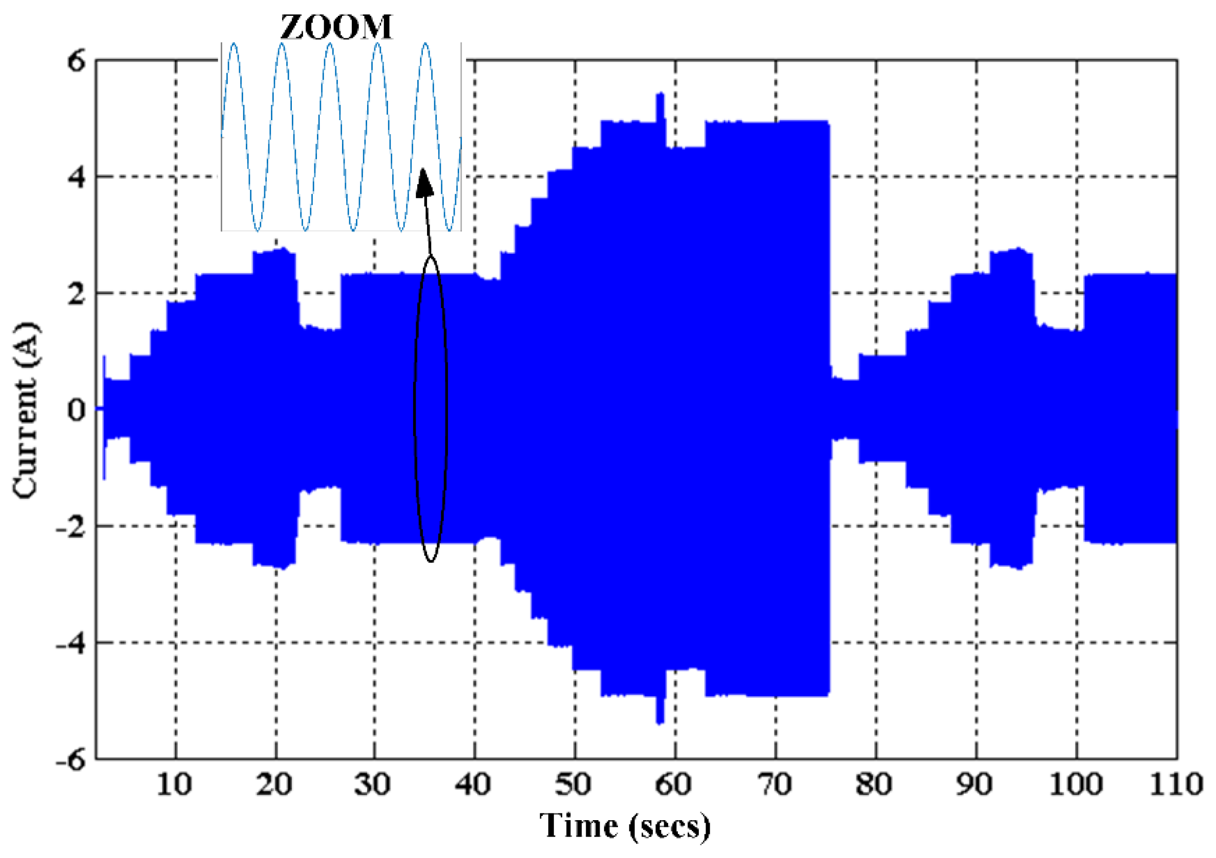
4.1. Proposed Sensor-less Configuration
4.2. Configuration with Sensors
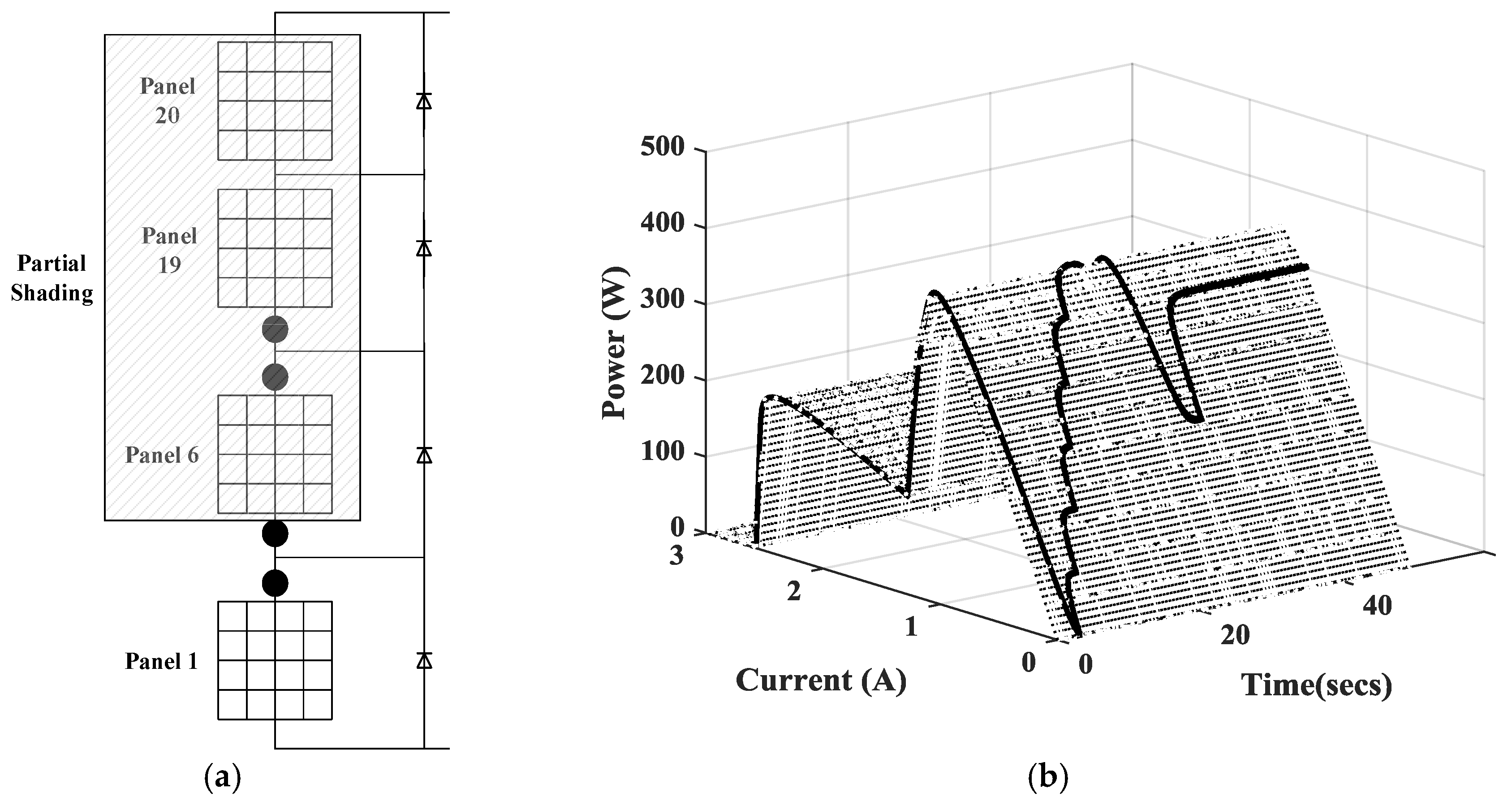
4.3. Proposed Sensor-Less Configuration under Partial Shading
4.4. Simulation Evaluation
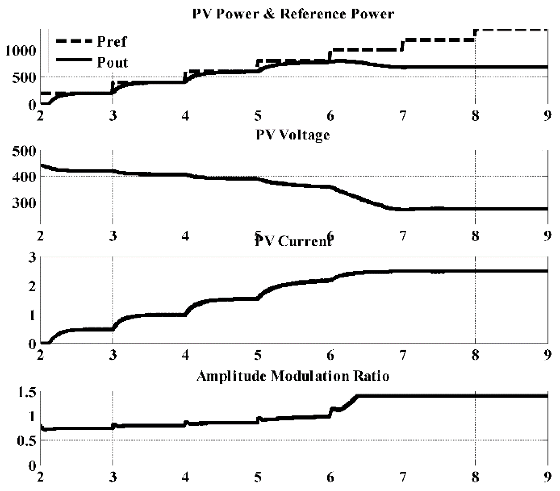
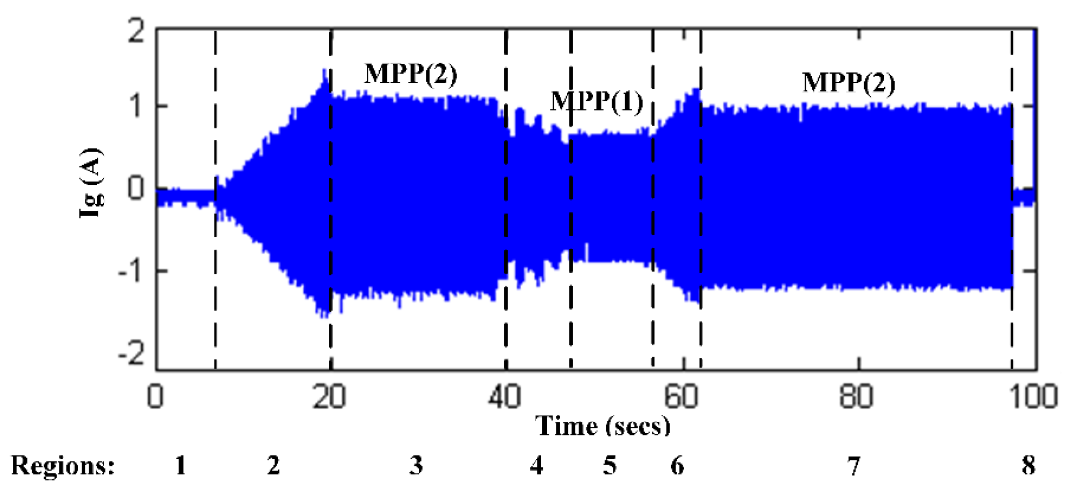
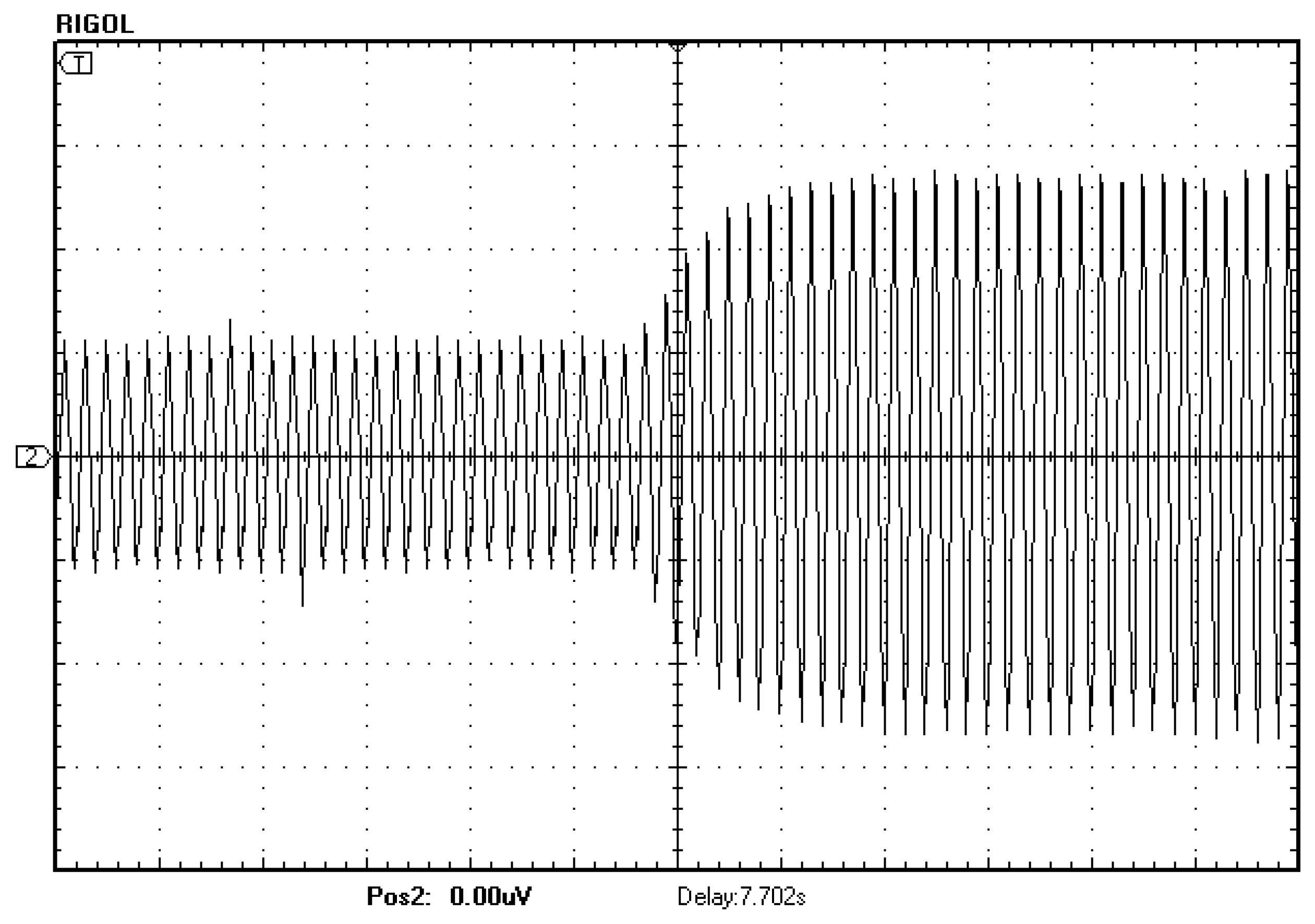
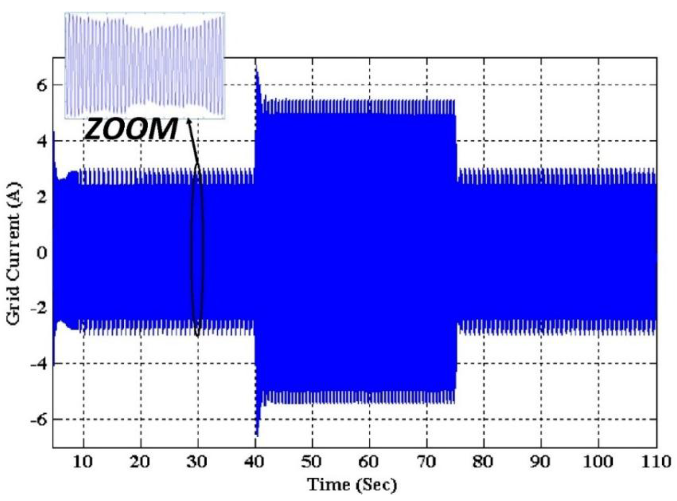
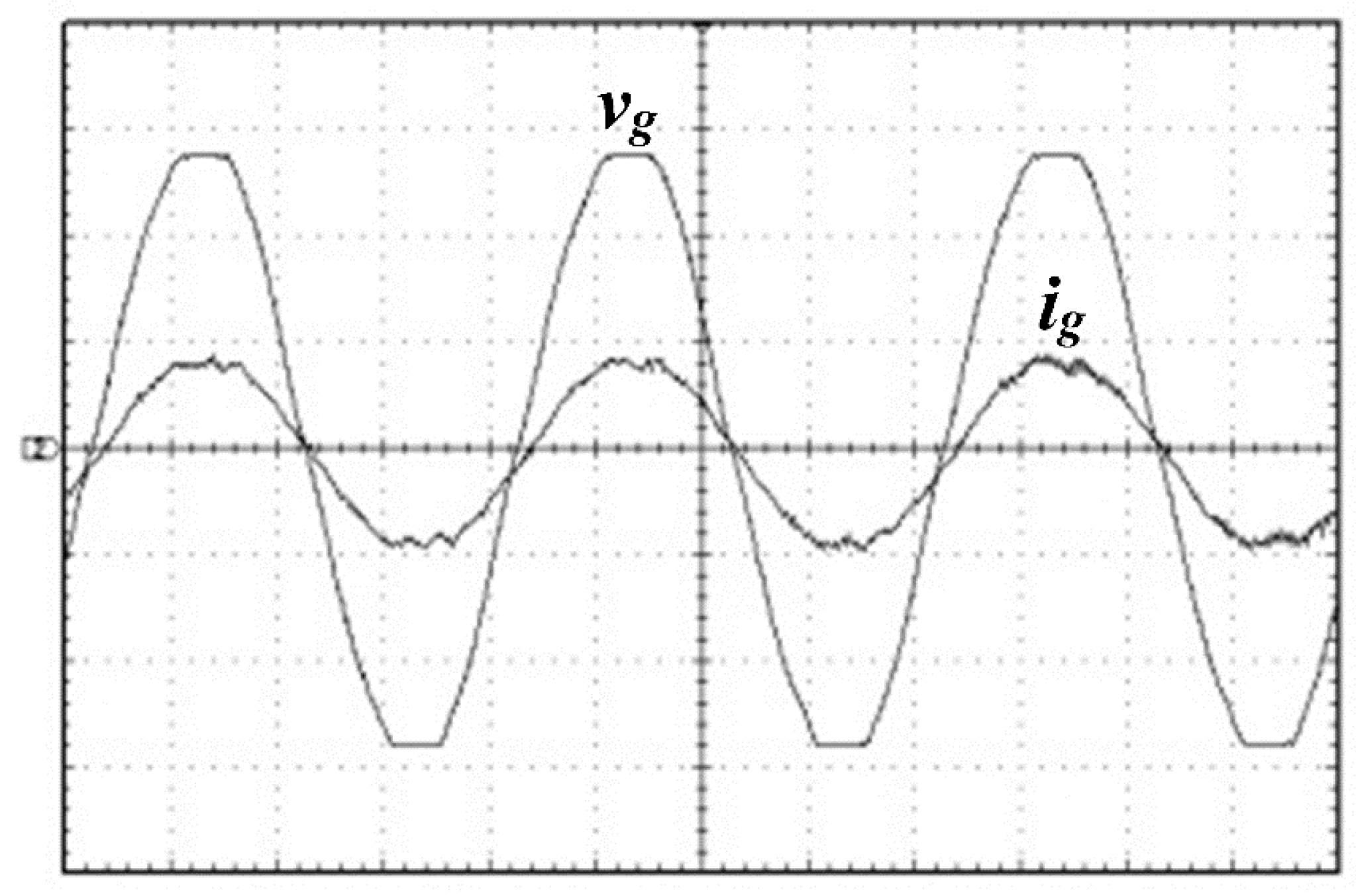
5. Experimental Results
6. Conclusions
Acknowledgments
Author Contributions
Conflicts of Interest
References
- Kjaer, S.B.; Pedersen, J.K.; Blaabjerg, F. A Review of single-phase grid-connected inverters for photovoltaic modules. IEEE Trans Ind. Appl. 2005, 41, 1292–1306. [Google Scholar] [CrossRef]
- Marzband, M.; Parhizi, N.; Savaghebi, M.; Guerrero, J.M. Distributed smart decision-making for a multimicrogrid system based on a hierarchical interactive architecture. IEEE Trans. Energy Convers. 2015, 99, 1–12. [Google Scholar] [CrossRef]
- Marzband, M.; Azarinejadian, F.; Savaghebi, M.; Guerrero, J.M. An optimal energy management system for islanded microgrids based on multiperiod artificial bee colony combined with Markov chain. IEEE Syst. J. 2015, 99, 1–11. [Google Scholar] [CrossRef]
- Marzband, M.; Parhizi, N.; Adabi, J. Optimal energy management for stand-alone microgrids based on multi-period imperialist competition algorithm considering uncertainties: Experimental validation. Int. Trans. Electr. Energy Syst. 2015. [Google Scholar] [CrossRef]
- Marzband, M.; Yousefnejad, E.; Sumper, A.; Domínguez-García, J.L. Real time experimental implementation of optimum energy management system in standalone microgrid by using multi-layer ant colony optimization. Int. J. Electr. Power Energy Syst. 2015, 75, 265–274. [Google Scholar] [CrossRef] [Green Version]
- Rahim, N.A.; Selvaraj, J.; Krismadinata. Hysteresis current control and sensorless MPPT for grid-connected photovoltaic systems. In Proceedings of the IEEE International Symposium on Industrial Electronics, Vigo, Spain, 4–7 June 2007; pp. 572–577.
- Kitano, T.; Matsui, M.; Xu, D.H. Power sensor-less MPPT control scheme utilizing power balance at DC link-system design to ensure stability and response. In Proceedings of the 27th Annual Conference of the IEEE Industrial Electronics Society, Denver, CO, USA, 29 November–2 December 2001; pp. 1309–1314.
- Park, S.S.; Jinda, A.K.; Gole, A.M.; Park, M.; Yu, I.K. An optimized sensorless MPPT Method for PV generation system. In Proceedings of the 2009 Canadian Conference on Electrical and Computer Engineering, St. John's, NL, USA, 3–6 May 2009; pp. 720–724.
- Wu, L.B.; Zhao, Z.M.; Liu, J.Z.; Shu, L.; Yuan, L.Q. Modified MPPT strategy applied in single-stage grid-connected photovoltaic system. In Proceedings of the Eighth International Conference on Electrical Machines and Systems, Nanjing, China, 29 September 2005; pp. 1027–1030.
- Ciobotaru, M.; Teodorescu, R.; Blaabjerg, F. Control of single-stage single-phase PV inverter. In Proceedings of the 2005 European Conference on Power Electronics and Applications, Dresden, Germany, 11–14 September 2005.
- Phani Kiranmai, K.S.; Veerachary, M. A single-stage power conversion system for the PV MPPT application. In Proceedings of the IEEE International Conference on Industrial Technology, Mumbai, India, 15–17 December 2006; pp. 2125–2130.
- Jain, S.; Agarwal, V. Comparison of the performance of maximum power point tracking schemes applied to single-stage grid-connected photovoltaic systems. IET Electr. Power Appl. 2007, 1, 753–762. [Google Scholar] [CrossRef]
- Liu, F.; Zhou, Y.; Yin, J.; Duan, S. An improved MPPT arithmetic and grid-connected control strategy for single-stage three-phase PV converter with LCL filter. In Proceedings of the 3rd IEEE Conference on Industrial Electronics and Applications, Singapore, Singapore, 3–5 June 2008; pp. 808–813.
- Li, D.; Gao, G.; Loh, P.C.; Wang, P.; Tang, Y. Transient maximum power point tracking for single-stage grid-tied inverter. IEEE Energy Convers. Congr. Expo. 2009, 313–318. [Google Scholar] [CrossRef]
- Wu, L.B.; Zhao, Z.M.; Liu, J.Z. A single-stage three-phase grid-connected photovoltaic system with modified MPPT method and reactive power compensation. IEEE Trans. Energy Convers. 2007, 22, 881–886. [Google Scholar]
- Yu, W.L.; Lee, T.-P.; Wu, G.-H.; Chen, Q.S.; Chiu, H.-J.; Lo, Y.-K.; Shih, F. A DSP-based single-stage maximum power point tracking PV inverter. In Proceedings of the 2010 Twenty-Fifth Annual IEEE Applied Power Electronics Conference and Exposition (APEC), Palm Springs, CA, USA, 21–25 February 2010; pp. 948–952.
- Lacerda, V.S.; Barbosa, P.G.; Braga, H.A.C. A single-phase single-stage, high power factor grid-connected PV system, with maximum power point tracking. In Proceedings of the 2010 IEEE International Conference on Industrial Technology (ICIT), Vina del Mar, Spain, 14–17 March 2010; pp. 871–877.
- Patel, H.; Agarwal, V. MPPT scheme for a PV-fed single-phase single-stage grid-connected inverter operating in CCM with only one current sensor. IEEE Trans. Energy Convers. 2009, 24, 256–263. [Google Scholar] [CrossRef]
- Elsaharty, M.A.; Hamad, M.S.; Ashour, H.A. Digital hysteresis current control for grid-connected converters with LCL filter. In Proceedings of the 37th Annual Conference on IEEE Industrial Electronics Society, Melbourne, Australia, 7–10 November 2011; pp. 4685–4690.
- Hu, H.B.; Harb, S.; Kutkut, N.H.; Shen, Z.J.; Batarseh, I. A single-stage microinverter without using eletrolytic capacitors. IEEE Trans. Power Electron. 2013, 28, 2677–2687. [Google Scholar] [CrossRef]
- Villalva, M.G.; Gazoli, J.R.; Filho, E.R. Comprehensive approach to modeling and simulation of photovoltaic arrays. IEEE Trans. Power Electron. 2009, 24, 1198–1208. [Google Scholar] [CrossRef]
- Pouresmaeil, E.; Montesinos-Miracle, D.; Gomis-Bellmunt, D. Control scheme of three-level h-bridge converter for interfacing between renewable energy resources and AC grid. In Proceedings of the 14th European Conference on Power Electronics and Applications, Birmingham, UK, 30 August–1 September 2011; pp. 1–9.
- Elsaharty, M.A.; Ashour, H.A. Realization of DC-bus sensor-less MPPT technique for a single-stage PV grid-connected inverter. In Proceedings of the 23rd International Conference and Exhibition on Electricity Distribution, Lyon, France, 15–18 June 2015; p. 204.
- Nousiainen, L.; Puukko, J.; Mäki, A.; Messo, T.; Huusari, J.; Jokipii, J.; Viinamäki, J.; Lobera, D.T.; Valkealahti, S.; Suntio, T. Photovoltaic generator as an input source for power electronic converters. IEEE Trans. Power Electron. 2013, 28, 3028–3038. [Google Scholar] [CrossRef]
- Urtasun, A.; Sanchis, P.; Marroyo, L. Adaptive voltage control of the DC/DC boost stage in PV converters with small input capacitor. IEEE Trans. Power Electron. 2013, 28, 5038–5048. [Google Scholar] [CrossRef]
- Khanna, R.; Zhang, Q.H.; Stanchina, W.E.; Reed, G.F.; Mao, Z.H. Maximum power point tracking using model reference adaptive control. IEEE Trans. Power Electron. 2014, 29, 1490–1499. [Google Scholar] [CrossRef]
- Liu, L.; Li, H.; Xue, Y.; Liu, W. reactive power compensation and optimization strategy for grid-interactive cascaded photovoltaic systems. IEEE Trans. Power Electron. 2015, 30, 188–202. [Google Scholar]
- Pouresmaeil, E; Jorgensen, B.N.; Veje, C.; Catalao, J.P.S. A flexible control strategy for integration of DG sources into the power grid. In IEEE Proceedings of the Australasian Universities Power Engineering Conference (AUPEC), Perth, Australia, 28 September–1 October 2014; pp. 1–6.
- Mehrasa, M.; Adabi, E.; Pouresmaeil, E.; Adabi, J. Passivity-based control technique for integration of DG resources into power grid. Int. J. Electr. Power Energy Syst. 2014, 58, 281–290. [Google Scholar] [CrossRef]
- Mehrasa, M.; Pouresmaeil, E.; Mehrjerdi, H.; Jørgensen, B.N.; Catalao, J.P.S. Control technique for enhancing the stable operation of distributed generation units within a microgrid. Energy Convers. Manag. 2015, 97, 362–373. [Google Scholar] [CrossRef]
- Pouresmaeil, E.; Akorede, M.F.; Hojabri, M. A hybrid algorithm for fast detection and classification of voltage disturbances in electric power systems. Eur. Trans. Electr. Power 2011, 21, 555–564. [Google Scholar] [CrossRef]
- Elsaharty, M.A.; Ashour, H.A. Passive L and LCL filter design method for grid-connected inverters. In Proceedings of the IEEE Innovative Smart Grid Technologies, Kuala Lumpur, Malaysia, 20–23 May 2014.


| Parameter | Value |
|---|---|
| Vg | 220 Vrms |
| Number of series PV modules | 20 |
| PV array total maximum power | 800 W |
| L1 | 80 mH |
| Cdc | 10 mF |
| mamax | 0.98 |
| Settlement range | ±0.002 |
| Δma | 0.005 |
| algorithm sampling rate | 0.1 s |
| Ki Sensorless configuration | 8.0 |
| Kp Sensored configuration (Voltage control loop) | 0.5 |
| Ki Sensored configuration (Voltage control loop) | 2.2 |
| Kp Sensored configuration (Current control loop) | 0.4 |
| Ki Sensored configuration (Current control loop) | 8.0 |
| Sensorless configuration reference power increment | 70 W |
| Sensored configuration reference voltage increment | 1 V |
| Tracking Time | Current Oscillations | Sensors | Configuration |
|---|---|---|---|
| 26 s | 0 | 2(Vg, Ig) | Proposed (Figure 9) |
| 0.3 s | 3.3% | 4(Vdc, Idc, Vg, Ig) | Classical (Figure 1b) |
| Parameter | Value |
|---|---|
| Vg | 220 Vrms |
| PV Panel Type | LORENTZ LC175-24M |
| Number of parallel PV Panels | 2 |
| PMPP/panel | 175 W at 1000 W/m2 |
| VMPP | 35 V at 1000 W/m2 |
| L1 | 4 mH |
| Cdc | 10 mF |
| Transformer ratio | 7/230 V |
| Switching frequency & Current controller sampling frequency | 10 kHz |
| Reference output power incremenet | 15 W |
| Algorithm sampling rate | 0.1 s |
© 2016 by the authors; licensee MDPI, Basel, Switzerland. This article is an open access article distributed under the terms and conditions of the Creative Commons by Attribution (CC-BY) license (http://creativecommons.org/licenses/by/4.0/).
Share and Cite
Elsaharty, M.A.; Ashour, H.A.; Rakhshani, E.; Pouresmaeil, E.; Catalão, J.P.S. A Novel DC-Bus Sensor-less MPPT Technique for Single-Stage PV Grid-Connected Inverters. Energies 2016, 9, 248. https://doi.org/10.3390/en9040248
Elsaharty MA, Ashour HA, Rakhshani E, Pouresmaeil E, Catalão JPS. A Novel DC-Bus Sensor-less MPPT Technique for Single-Stage PV Grid-Connected Inverters. Energies. 2016; 9(4):248. https://doi.org/10.3390/en9040248
Chicago/Turabian StyleElsaharty, Mohamed A., Hamdy A. Ashour, Elyas Rakhshani, Edris Pouresmaeil, and João P. S. Catalão. 2016. "A Novel DC-Bus Sensor-less MPPT Technique for Single-Stage PV Grid-Connected Inverters" Energies 9, no. 4: 248. https://doi.org/10.3390/en9040248