Measuring the Actual Energy Cost Performance of Green Buildings: A Test of the Earned Value Management Approach

Abstract

Reduced energy consumption is a key aspect of the green building. Nonetheless, research indicates that there is a performance gap between the predicted and the actual energy performance once buildings are occupied, which implies a cost deviation from the anticipated energy cost performance. However, the cost deviation also might result from lower or higher energy rates than expected. As an appropriate research methodology for existing theory testing, case study research strategy was adopted to empirically examine the earned value management (EVM) approach to measure the actual life cycle cost performance of energy in green buildings. With slight methodological and terminological adaptations, it is found that the EVM approach can be applied to conduct a holistic cost performance measurement of the actual energy consumption in green buildings. The strength of the earned value approach is that it allows for detecting whether the energy cost saving or overrun results from lower or higher energy consumption, or from actual energy rate variations. The earned value approach allows for quantifying each cost variance independently, which is a significant aspect of actual energy cost performance measurement in green buildings.

1. Introduction

A key message in a report issued by the United Nations Environment Programme [1] indicates that the building sector is the largest single contributor to greenhouse gas emissions and around one-third of global energy end use is being consumed in buildings. It is also highlighted in the report that the building sector has a significant potential to use resources more efficiently. Aligned with the concept of sustainable development, the green building is being promoted as a high potential solution to reduce gas emissions and natural resource depletion. Intrinsically, the green building is designed considering the economic dimension of sustainability, and therefore, has a wide spectrum of benefits which are typically assessed from the life cycle perspective [2,3,4]. In addition to reduced water and natural resource consumption, improved health and productivity, improved indoor air quality [2,5], among others, reduced energy consumption is perceived as a significant benefit associated with the green building, an energy saving ranges from 25% to 70% is empirically argued in the literature [3,6,7,8,9,10].

However, it is claimed that buildings sometimes do not perform as predicted [11,12,13,14,15,16]. In a paper, de Wilde [12] argues that there is a significant variation between the predicted energy performance and the actually measured energy use while buildings under operation, the author highlights several factors related to design, construction, and building operation as root causes for this “performance gap” as termed in the literature [11,12,17]. In a relatively old study, Norford et al. [18] found that the actual energy consumption was around 160% more than the predicted performance in a low energy office building. Salehi et al. [17] reported 60% higher energy consumption than predicted in a green building. Torcellini et al. [10] studied six high performance buildings and found that the six buildings are using from 25% to 70% lower energy than code-compliant buildings, but they observed that the six buildings are using more energy than the design simulations. On a larger scale study, Turner and Frankel [19] measured the actual energy consumption for 121 green buildings certified under the LEED (Leadership in Energy and Environmental Design) and found that more than half of the buildings are deviating from design predictions by more than 25%. In the study some green buildings are using 250% more energy than predicted.

However, similar performance gaps in other performance areas also were highlighted in the literature. In a study conducted by the U.S. General Service Administration [20] to evaluate the performance of 22 green buildings, it is found that five green buildings recorded 25% higher maintenance cost than the United States national average of commercial buildings, three buildings recorded higher energy consumption, and six buildings used more water than the United States national average. Similarly, Fowler and Rauch [21] evaluated 12 sustainably design buildings, they found that three buildings recorded higher maintenance costs than the industry baseline in the United States, one building has higher energy costs, in addition to two buildings used more water than the baseline. Therefore, it is necessary to track the actual economic performance of green buildings to quantify the magnitude of such gaps in performance, wherever exists.

In this research, the EVM is examined in a new context, which is building operating phase, to measure the actual end use energy cost performance of green buildings. The EVM is a widely recognized cost performance measurement technique for projects in various industrial sectors, it allows an early detection of cost performance issues [22,23]. As a methodology used to objectively measure the actual cost performance in projects [22,24], the EVM allows to calculate a set of performance indicators and metrics to quantify the magnitude of the cost deviation from a predefine cost performance baseline [24,25,26]. This research aims to examine the earned value approach in measuring the actual energy cost performance of green buildings and it was designed to answer the following questions:

RQ. 1  

Can the actual energy cost performance in green buildings be measured using the earned value approach?

RQ. 2  

How can the earned value of energy be measured throughout the life cycle of the green building?

RQ. 3  

What are the methodological implications associated with using the EVM to measure the actual energy cost performance in green buildings?

2. Background Information

2.1. The Concept of the Green Building

Introduced in the early nineties [4], the concept of the green building is perceived as a high potential solution to reduce the negative impacts on the environment through using less natural resources to build and operate. The green building is being discussed in the literature under different terms: green buildings, sustainable buildings, high performance buildings, sustainable construction, green construction, high performance construction [2,4,13]. Energy and water saving, less greenhouse gas emissions, reduced material and natural resource consumption, in addition to improved internal indoor environment are major benefits associated with the green building [3,4]. Yudelson [3] argue that the typical energy and water saving in green buildings ranges from 30% to 50%. Kats et al. [2] found that green buildings save energy on an average of 30% compared to conventional (non-green) buildings.

The key concept of the green building is to utilize renewable energy sources to reduce energy demand in buildings [4,27,28]. Proper building orientation, efficiently insulated and glazed building envelope, more efficient electrical appliances, among others, are various design strategies can be implemented to reduce energy demand in buildings [5,28,29]. Levine et al. [28] argue that cooling and heating energy demand in buildings can be reduced from 50% to 75% through implementing passive design strategies for buildings. The passive design is a term refers to improvements of building envelope to reduce the total energy demand in buildings [30]. On-site energy production from renewable energy sources such as solar, wind, and geothermal (heat from the earth) is another key aspect of the green building. Supported by passive design strategies, on-site energy production can cover a higher percentage of the total energy demand in buildings [5], allowing the balance energy demand to be completely covered from renewable energy sources [28].

Yet, there are no globally recognized standard criteria to assess the performance of the green building and to rate a building as green. The assessment methods of green building performance are divers and locally applied. Around 60 countries from all over the word [4] have their own rating systems and evaluation criteria to promote the green building. Leipziger [31] compared 17 building energy assessment systems in 10 countries and concluded that the performance measurement systems are designed to largely match local priorities, the author further argue that more work is still required to consistently clarify what energy efficiency implies and how it can be assessed.

2.2. Earned Value Management (EVM)

The EVM is a project management technique used to monitor and control projects cost and time schedule in an integrated manner [25,26]; it is a management methodology used to objectively measure the cost performance of a project and to predict its future performance [22]. Popescu and Charoenngam [32] in their book entitled Project Planning, Scheduling, and Control in Construction: An Encyclopedia of Terms and Applications, define the earned value management as: “the performance measurement to report the status of a project in terms of both cost and time at a given data date”. The EVM helps in calculating performance metrics not available by merely comparing the actual costs against the planned costs [33]. The earned value analysis is based on identifying three principal performance measurement parameters which are: planned value (PV), earned value (EV), and actual cost (AC) [25,26]. Based on these three cost parameters, an extensive list of performance indicators and metrics can be calculated to report projects performance in term of cost and time progress [22,25,34].

The earned value (EV) is the key parameter in measuring cost performance of projects; it is the common parameter used to measure both cost and time performance [22,24,25,26]. From the ANSI standard ANSI/EIA-748-B-2007 [35], a clear definition can be cited for the earned value (EV) as: “the value of completed work expressed in terms of the budget assigned to that work”. Fleming and Koppelman [24] suggest that the earned value is what physically obtained from the money spent. However, various definitions can be cited from the literature and all of them imply similar meanings and descriptions.

2.2.1. Concept and Origin

As a method for performance measurement of cost and time progress of projects, the historical evolution of EVM can be traced back to 1800s, but its current form and function was developed and proposed by the United States Air Force in 1960s and named “the cost/schedule planning and control system” [24,36]. In 1967, it was adopted by the United States Department of Defense as a policy and it was renamed to “cost/schedule control systems criteria (C/SCSC)” [24,26,36,37].

The EVM has gained momentum and became an industry standard to track progress and cost performance in construction projects [22,25,26]. According to Fleming and Koppelman [24], the traditional cost performance measurement approach in which the actual cost is compared against the planned cost is often misleading and does not allow to accurately measure the actual cost performance of projects, the authors contend that the traditional cost performance measurement approach is a two dimensional approach; it does not consider the third dimension which is the value of the work performed as a principal parameter to measure the actual cost performance of projects.

The key concept of the EVM revolves around that comparing the actual cost with the planned cost does not provide meaningful information about the budget status and the actual spending [22,25,26]. This is because that the project may deviate from its initial plan, and consequently, the executed work value may be less or more than the planned work. Figure 1 is a graphic representation of the EVM concept and parameters.

2.2.2. Performance Parameters and Performance Indicators

In cost performance measurement, the earned value (EV) is compared to the accrued actual cost (AC) up to a specific time period, the resultant cost variance (CV) is a cost performance metric used to quantify the amount of cost deviation from the cost performance baseline [22,24]. Comparing the earned value (EV) with actual cost (AC) dissolves the effects of time schedule variations which are totally ignored by comparing the actual cost with the planned costs [24,35]. The cost variance (CV) is calculated using Equation (1) as follow [22,35]:

Cost variance (CV) = Earned value (EV) − Actual cost (AC)

(1)

The cost variance (CV) can be expressed as a percentage using Equation (2) as follow [22,26]:

Cost variance percentage (CV%) = Cost variance (CV)/Earned value (EV) × 100

(2)

The cost variance (CV) quantifies the amount of cost deviation whether it is positive or negative but it does not inform the magnitude of the cost saving or overrun, therefore, the cost performance index (CPI) is typically calculated. The cost performance index (CPI) is calculated by dividing the earned value (EV) of the work performed by its actual cost (AC) for the same time period. Equation (3) is typically used to calculate the cost performance index (CPI) [26,33]:

Cost performance index (CPI) = Earned value (EV)/Actual cost (AC)

(3)

The CPI measures the cost efficiency of projects and helps in determining the magnitude of the cost deviation from the cost baseline. Typically, a CPI equals 1.0 implies a favorable cost performance, while a CPI less than 1.0 indicates a poor cost performance [22,24,25,26,35]. The CPI can be calculated periodically (yearly, monthly, weekly, and daily) to forecast long term performance trends [33].

Likewise, the time performance is measured through calculating the schedule variance (SV) which is the difference between the earned value (EV) and the planned value (PV). The schedule variance (SV) is a metric used to quantify how much the project is running ahead or behind the time schedule [22,24,25,26]. The schedule variance (SV) is calculated using Equation (4) as follow [22,26]:

Schedule variance (SV) = Earned value (EV) − Planned value (PV)

(4)

It is worth mentioning that the schedule variance (SV) is based on monetary values to quantify the deviation from the time schedule; it does not report the schedule variance in term of time units. The schedule variance (SV) can be expressed as a percentage using Equation (5) as follow [22,26]:

Schedule variance percentage (SV%) = Schedule variance (SV)/Planned value (PV)

(5)

The schedule variance percentage (SV%) measures how much more or less work performed in reference to the initial project time plan. Similar to the concept of cost performance index (CPI), schedule performance index (SPI) is also calculated to report the magnitude of work deviation from the initial project time plan. The SPI is a metric used to measure time efficiency in projects, it can be calculated using Equation (6) as follow [22,26]:

Schedule performance index (SPI) = Earned Value (EV)/Planned value (PV)

(6)

Similar to the cost performance index (CPI), the schedule performance index (SPI) is reported in reference to 1.0, an SPI less than 1.0 indicates unfavorable condition and means that less work executed than planned.

3. Research Methodology

3.1. Research Strategy

The EVM is a well-developed theory and it is being implemented in practice [22,23]. In this research, the EVM was examined in a new context which is building operating phase, and therefore, the research was designed and implemented as existing theory test. In existing theory testing, several research methodology scholars [38,39,40,41,42] recommend to use case study as the research strategy. Case study is an intensive research approach appropriate to answer wide research questions in depth by explaining how a process develops and works within a case [40]. It is often used when the research addresses contemporary issues over which the investigator has little or no control [38,39,43]. Case study research focuses on empirical testing [43], and it allows to investigate and understand emerging problems to propose practical solutions [40].

3.2. Sampling

Sampling refers to the process of selecting a representative sample from a larger population, from which data are collected to make the conclusions generalizable for the whole population [39,44]. The issue of sampling was investigated by reviewing what research methodology scholars say about the subject matter. There is a consensus among case study research methodology scholars that non-probability sampling is recommended for case study research; they suggest that samples are selected purposively because they are information-rich case studies that allow deep investigation and analysis to answer the research questions [38,39,42,45,46].

A single case is often used in case study strategy [38,40,42,45]. A single case is used because it is a critical, extreme, or unique case [38,45,47], or it is a typical case representing a group of cases [39,48]. Yin [38] contends that a single case study is a common approach in case study research, in page 52 he says:

Overall, the single-case design is eminently justifiable under certain conditions where the case represents (a) a critical test of existing theory, (b) a rare or unique circumstance, or (c) a representative or typical case, or where the case serves a (d) revelatory or (e) longitudinal purpose.

The characteristics of the research support the selection of a single case study approach to answer the research questions. This is because, first, the unit of analysis in the research is a green building under operation, and intrinsically, the characteristics of green buildings are typical, which means that the results can be theoretically generalized for a larger population. Second, the research aims to answer broad research questions about how a process develops within real-life context, a single case study approach allows an in-depth investigation to answer the research questions [38,45]. Third, but most importantly, the research neither aims to test popularity of a phenomenon nor causal relationship between variables which is a major characteristic of the research.

3.3. Case Study Description

The case study which was analyzed in the research is the Malaysia Energy Center formerly known as ZEO (Zero Energy Office) Building, it is the first officially certified green building in Malaysia and currently known as GEO (Green Energy Office) Building [49]. Located near Kuala Lumpur, the building was commissioned in 2008 as a showcase green building in Malaysia. The building scored full points under the energy efficiency and innovation criteria in the Green Building Index (GBI) rating system [49].

Table 1. Case Study Information.

No.	Description
1	Building name	GEO Building
2	Building location	Kuala Lumpur-Malaysia
3	Building type	Commercial building
4	Building function	Office building
5	Green certification level	GBI-Certified
6	Green certification year	2009
7	Building commissioning date	2008
8	Building gross area	4300 m2
9	Building Energy Index (BEI) based on design simulation	65 kWh/m2/year
10	BEI based on actual energy consumption	39 kWh/m2/year

shows the case study information and attributes.

GEO Building was designed and constructed adopting green technologies and eco-friendly features such as 100% daylight in the offices, double glazing and insulation, thermal energy storage, energy efficient lighting, rainwater harvesting system, building energy management system (BEMS), floor slab cooling system, in addition to a building integrated photovoltaic (BIPV) system installed in the building with a capacity of 92 kWp. The BIPV system generates 120,000 kWh/year or 50% of the building energy demand and it is connected to the national grid via net-metering to export surplus electricity [50]. Figure 2 is a general view of the case study.

The GEO Building was designed to achieve a building energy index (BEI) of 65 kWh/m²/year, which is far below the average BEI of a typical office building in Malaysia which ranges from 250 to 300 kWh/m²/year [51,52]. Calculated based on actual energy consumption, the BEI was equal 40 kWh/m²/year in 2014 [50].

3.4. Data Collection

To answer the posed research questions in the research, two types of data were required. The first type related to energy cost performance baseline. The cost performance baseline is the backbone of the earned value analysis [22,25,26]; it forms the reference against which the actual cost performance is measured and reported [24]. The second type of the required data related to the actual life cycle cost of energy for the performance measurement period. Within the context of the EVM, the performance measurement period refers to the period during which the cost performance measurement is conducted [22]. For the case study, it covers the building operating period starting from building commissioning date (2008) up to the date up to which actual record for building energy consumption and cost are available which is the end of 2014.

The actual energy consumption and cost data for the case study are available online through the Malaysian Green Technology Corporation official portal [50]. The actual building performance data contain records for the actual monthly building energy consumption and cost. The actual data were available up to the year 2014, and hence, it is used as the data date up to which the performance is measured.

Since its commissioning in 2008 and up to the end of 2014, the building consumed 1,175,772 kWh of energy, this corresponds to an actual energy cost equals $142,746. The average annual energy consumption equals 167,967 kWh/year while the monthly average is 13,997 kWh/month. The building energy index (BEI) is being calculated annually and published online by the building owners, the average BEI for the building since its commissioning is 39 kWh/m²/year as illustrated in Figure 3.

Table 2. Actual energy consumption and cost data.

Year	Annual Energy Consumption (kWh/Year)	Average Monthly Consumption (kWh/Month)	Building Energy Index (BEI) (kWh/m2/Year)	Actual Energy Cost ($/Year)
2008	243,900	20,325	57	29,611
2009	151,284	12,607	35	18,367
2010	140,160	11,680	33	17,016
2011	127,068	10,589	30	15,427
2012	165,960	13,830	39	20,149
2013	175,224	14,602	41	21,273
2014	172,176	14,348	40	20,903
Total	1,175,772 kWh	-	-	$142,746

shows the actual annual energy consumption, the actual annual energy costs, the monthly average consumption, and the BEI for the case study.

The annual BEI for the case study was calculated by dividing the total annual energy consumption over the building gross area which equals 4300 m². The BEI, also known as energy efficiency index (EEI) [53], or energy use intensity (EUI) [10,20], is a common performance indicator used to track and measure the total annual energy used in a building. It is expressed as kWh/m²/year and it can be calculated by dividing the total annual energy used in a building by its gross floor area measured in square meters [52,53].

All the cost data were available in the local currency of Malaysia, the average exchange rate for the year 2014 which was equal 3.91 RM/US$, according to the Central Bank of Malaysia [54], was used to convert all the cost data to the American dollar.

4. Energy Life Cycle Cost Baseline

4.1. Period of Analysis

Within the context of life cycle cost, the period of analysis refers to the period of time over which the life cycle cost of a building is analyzed [55,56,57]. The International Standard ISO 15686-5 [57] recommends that the estimated service life of a building should not be less than its design life. The service life of a building is determined by the period of time during which a building or its components satisfy the minimum acceptable level of performance [58]. Determining the service life of the building was essential to identify the time horizon over which the study is conducted. As a concrete structure, the service life of the case study is expected to extend for 60 years as a minimum [59]. Therefore, a period of 60 years was used as a time horizon for the analysis starting from the year 2008 to 2067 inclusive.

The main purpose of using the whole building life cycle as the period of analysis is to see how the period of analysis impacts the earned value parameters and results. The energy price inflation significantly impacts the estimated total life cycle budget of energy as discussed in the subsequent sections.

4.2. Energy Price Inflation

The inflation/deflation refers to the continuous increase/decrease in the general price level of goods and services [57,60]. According to the Department of Statistics Malaysia [61], the average price increase in energy was about 2.4% per year and it covers a period starting from 1981 to 2014. This rate was used in Equation (7) to project the estimated annual energy cost over the whole building life cycle [57,62]:

F = P(1 + e)ⁿ

(7)

where:

F	future value (nominal cost).
P	cost in the base year.
e	expected percentage of annual cost increase.
n	number of years between the base date and the occurrence of the cost.

4.3. Energy Cost Performance Baseline

The energy performance in buildings is measured against an absolute objective reference number determined based on a technical standard, or against a relative reference performance of peer buildings, sometimes referred to as industry baseline [21,53,63]. Leipziger [31] suggests that the absolute reference as a performance metric better suits policy formulation in which an end goal such as net zero energy is targeted, he, in contrast, argues that a relative reference allows measuring a building performance in reference to the market at large.

It is argued that a typical office building in Malaysia consumes energy, on average, from 250 to 300 kWh/m²/year [50,51]. However, there is no empirical evidence supports these figures and they are far above 135 kWh/m²/year which is the standard BEI set by the Code of Practice on Energy Efficiency and Use of Renewable Energy for Non-Residential Buildings (the Malaysian Standard MS1525:2007) [64,65,66]. In a research paper, Saidur [67] found that the BEI of office buildings in Malaysia is 130 kWh/m²/year based on data analyzed for 68 office buildings. As a national standard, the building energy index set by the Malaysian Standard (MS1525:2007) was used as a reference to develop the life cycle cost of energy for the case study.

According to the standard energy performance baseline, the total estimated end use annual energy consumption in the case study is around 580,500 kWh/year, calculated by multiplying the standard BEI, which equals 135 kWh/m²/year, by the building area, which equals 4300 m². This yields a total life cycle end use energy demand equals 34,830,000 kWh (580,500 kWh/year × 60 years).

The building commissioning year (2008) was used as the base year for energy life cycle cost baseline development. At the beginning of 2008, the applied electricity price tariff for commercial buildings was 0.099 $/kWh for all consumed energy quantity in a month [68]. Accordingly, the annual energy cost for the case study was calculated as follow:

Total annual energy cost = 580,500 kWh × 0.099 $/kWh = 57,470 $/year (rounded)

It is worth mentioning that the above calculations are based on the baseline performance and based on the assumption that the baseline energy use pattern in the case study will not change. However, investigating how the energy use pattern may change falls beyond the scope of the research since changing the energy use pattern does not affect the performance measurement approach which is examined in the research. , and hence, does not affect the findings of the research.

The above estimated annual energy cost is based on the energy prices which were effective in the base year (2008), to develop the energy life cycle cost baseline in the nominal terms (considering the energy price inflation), the average energy price inflation which equals 2.4% per year was used in Equation (7) to project the estimated annual energy budget over the building life cycle as shown in

Table 3. Estimated life cycle cost of energy for the case study (2008 as base year).

Estimated Annual Energy Cost ($/Year)
Year	Annual Energy Cost	Year	Annual Energy Cost	Year	Annual Energy Cost
2008	57,470	2028	92,346	2048	148,393
2009	58,849	2029	94,562	2049	151,954
2010	60,261	2030	96,831	2050	155,601
2011	61,707	2031	99,155	2051	159,335
2012	63,188	2032	101,535	2052	163,159
2013	64,705	2033	103,972	2053	167,075
2014	66,258	2034	106,467	2054	171,085
2015	67,848	2035	109,022	2055	175,191
2016	69,476	2036	111,639	2056	179,396
2017	71,143	2037	114,318	2057	183,702
2018	72,850	2038	117,062	2058	188,111
2019	74,598	2039	119,871	2059	192,626
2020	76,388	2040	122,748	2060	197,249
2021	78,221	2041	125,694	2061	201,983
2022	80,098	2042	128,711	2062	206,831
2023	82,020	2043	131,800	2063	211,795
2024	83,988	2044	134,963	2064	216,878
2025	86,004	2045	138,202	2065	222,083
2026	88,068	2046	141,519	2066	227,413
2027	90,182	2047	144,915	2067	232,871
Total estimated energy life cycle cost					$7,541,385

.

As can be seen in Table 3, the total estimated life cycle energy budget is around $7,541,385. This figure represents the baseline life cycle cost of energy based on the standard energy consumption as determined by the Malaysian Standard MS1525:2007. Figure 4 is a graphic representation of Table 3. It shows the cumulative life cycle cost of energy throughout the whole building life cycle which represents the life cycle cost performance baseline of energy.

5. Examining the Earned Value Approach to Measure Energy Cost Performance

Before proceeding further in the analysis, it is essential to redefine the earned value parameters, terminologies, and abbreviations considering the adopted life cycle approach in examining the EVM to measure the actual energy cost performance. The following modified terminologies and abbreviations were proposed and used in the research to distinguish and mark the earned value parameters in the life cycle context:

• Planned life cycle value, abbreviated PLCV: it is analogous to the planned value (PV), the PLCV is the time-phased life cycle budget of energy which used to develop the life cycle cost performance baseline; it is the cumulative life cycle budget of energy at any point in time throughout the building life cycle.
• Actual life cycle cost, abbreviated ALCC: it corresponds to the actual cost (AC); it is the actual amount of money spent on energy within a certain period of time throughout the building life cycle.
• Earned life cycle value, abbreviated ELCV: it is analogous to the earned value (EV), the ELCV is the equivalent monetary value of the consumed energy calculated in reference to the total estimated life cycle budget of energy.

The data date represents the time up to which the analysis is conducted; it covers the elapsed building operating period for which actual energy costs were recorded. For the case study, the data date is the end of 2014.

5.1. Performance Measurement Method

In the EVM, the earned value (EV) for the different work packages is determined based on an objective measurement method. The objective measurement method refers to using measurable criteria in determining work progress of the different work packages in the project [22,26,33], for example, physical progress percentage calculated based on actual produced quantities, time progress percentage determined based on the actual durations of the executed work, or resource usage percentage determined based on the actual resource consumption. The percentage which reflects the actual progress is multiplied by the budgeted cost of the respective work package to determine the earned value. However, it is noteworthy that the energy cost performance is not determined by work progress; rather it is determined by resource usage. Therefore, the actual energy consumption is examined as a measurement method to determine the earned life cycle value (ELCV) of energy.

5.2. Energy Earned Life Cycle Value

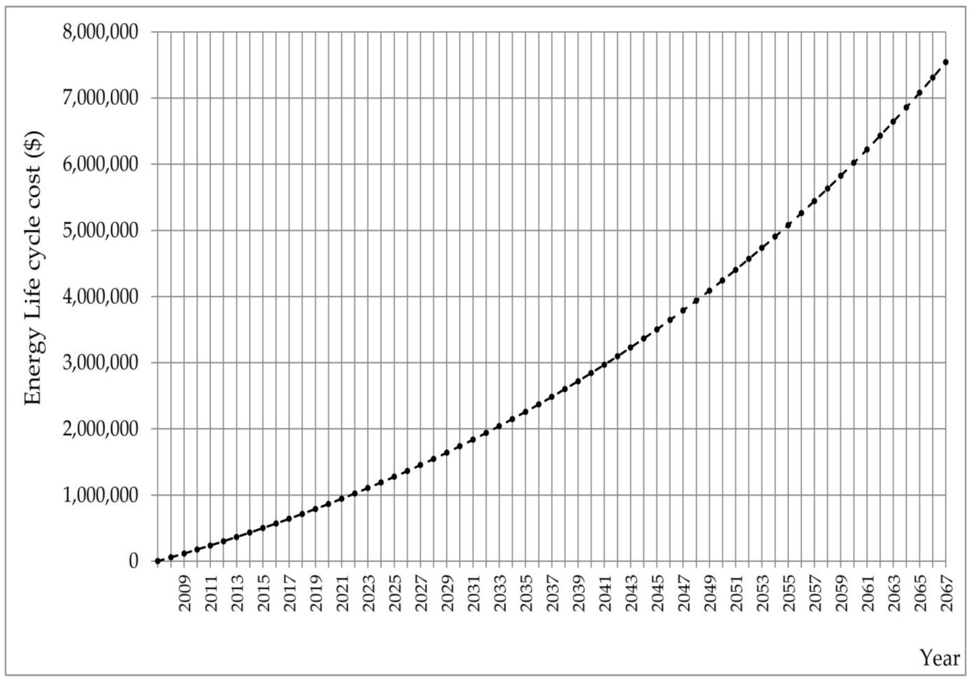
Based on the actual energy consumption percentage in the case study up to data date, the ELCV for energy equals $254,899, calculated by multiplying the actual energy consumption percentage (3.38%) by the total life cycle budget for energy which equals $7,541,385. The actual energy consumption percentage can be found by dividing the actual consumed energy up to data date which equals 1,175,772 kWh by the total end use energy demand in the building along its life cycle which equals 34,830,000 kWh.

The ELCV of energy under this measurement method also can be found by multiplying the actual consumed energy up to data date (1,175,772 kWh) by the average planned energy rate along the period of analysis which equals 0.217 $/kWh. The average planned energy rate can be found by dividing the total life cycle budget of energy ($7,541,385) over the total baseline energy demand (34,830,000 kWh). The resultant energy rate (0.217 $/kWh) represents the average escalated energy rate along the life cycle of the building. Multiplying the actual energy consumption (1,175,772 kWh) by the baseline average energy rate (0.217 $/kWh) equals $255,143. The difference between this figure and using the percentage is attributed to rounding; using unrounded figures yields exactly the same result.

The ELCV was calculated in reference to the budgeted life cycle cost of energy which is highly impacted by energy price inflation. The energy price inflation also highly influences the calculated ELCV and leads to an overestimated value. The exponential effect of energy price escalation on the total life cycle energy cost increases the calculated ELCV of energy. In other words, the future inflated energy cost is forwarded to impact the currently calculated ELCV. Therefore, using the above calculated ELCV to measure energy cost performance does not allow for fair and accurate cost performance measurement due to the significant effect of energy price escalation on the calculated ELCV.

The ELCV of energy can be more accurately determined using the annual baseline energy rates for the elapsed building operating period only. This is because the actual energy cost is determined based on the actual energy consumption and the actual applied rates by the utility service provider, and hence, calculating the ELCV of energy following the same approach allows fair and accurate cost variance calculations. It is worth reminding that the ELCV of energy is the corresponding value of the actual consumed energy quantity in reference to the estimated life cycle budget of energy, and hence, the baseline energy rates should be used in finding the earned life cycle value of energy.

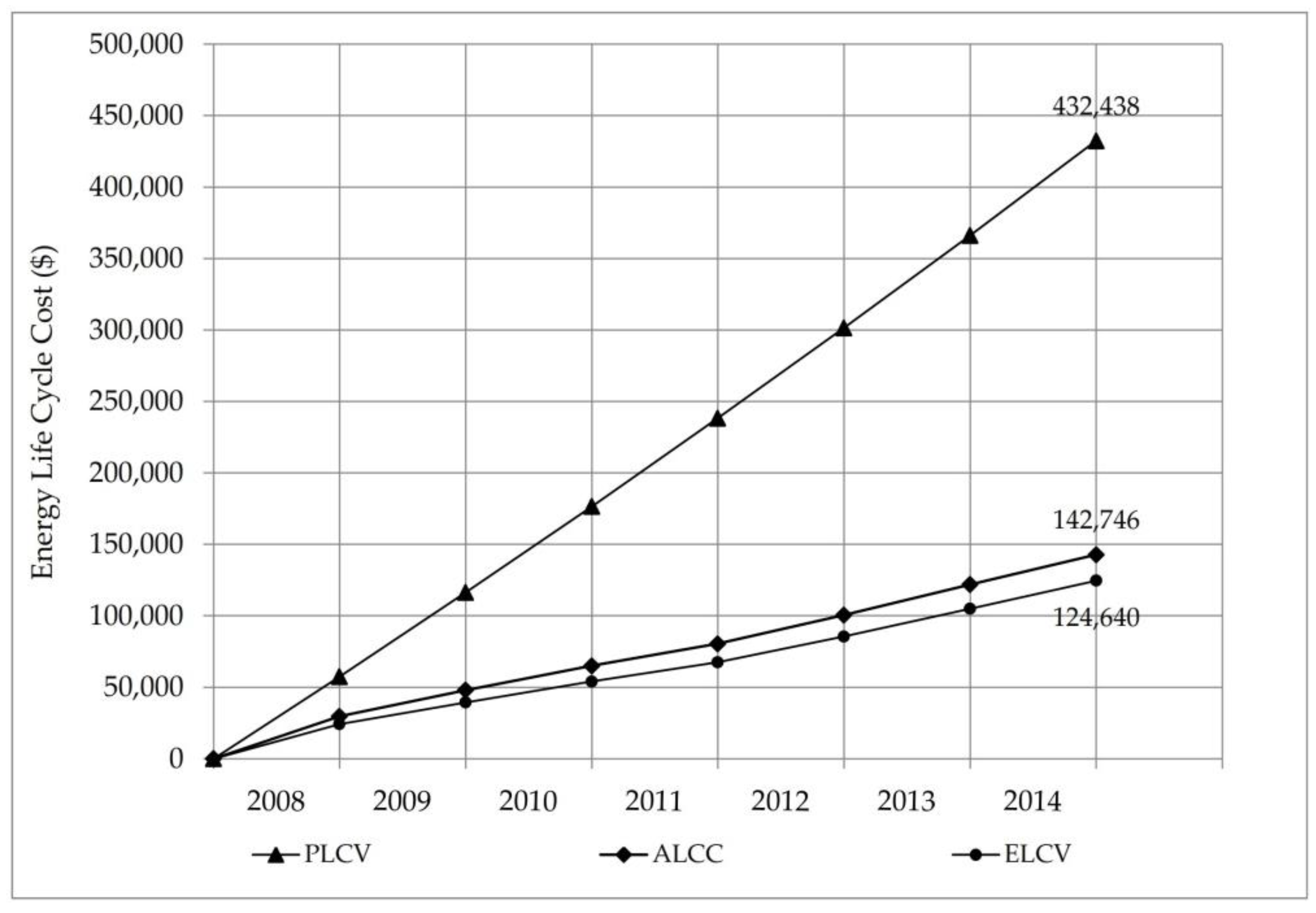
The annual baseline energy rates can be found by dividing the baseline energy cost in each year by the baseline energy consumption for the same year. This information is already available in the life cycle energy baseline. The calculated ELCV according to this approach equals $124,640 as illustrated in

Table 4. Energy earned value analysis parameters for the case study.

No.	Parameter	Value	Elapsed Building Operating Period
			2008	2009	2010	2011	2012	2013	2014
1	Baseline energy consumption (kWh)	Annual	580,500	580,500	580,500	580,500	580,500	580,500	580,500
		Cumulative	580,500	1,161,000	1,741,500	2,322,000	2,902,500	3,483,000	4,063,500
2	Planned life cycle value (PLCV)	Annual	57,470	58,849	60,261	61,707	63,188	64,705	66,258
		Cumulative	57,470	116,319	176,580	238,287	301,475	366,180	432,438
3	Actual energy consumption (kWh)	Annual	243,900	151,284	140,160	127,068	165,960	175,224	172,176
		Cumulative	243,900	395,184	535,344	662,412	828,372	1,003,596	1,175,772
4	Actual energy cost ($)	Annual	29,611	18,367	17,016	15,427	20,149	21,273	20,903
		Cumulative	29,611	47,978	64,994	80,421	100,570	121,843	142,746
5	Baseline energy rate ($/kWh)	Annual	0.099	0.101	0.104	0.106	0.109	0.111	0.114
6	Earned life cycle value (ELCV)	Annual	24,146	15,280	14,577	13,469	18,090	19,450	19,628
		Cumulative	24,146	39,426	54,003	67,472	85,562	105,012	124,640

. It is far below the calculated value using the actual energy consumption percentage which equals $254,899. This, however, significantly affects the cost variance and performance indices calculations.

Figure 5 is a graphic representation of Table 4 and illustrates the earned value parameters which were used to examine the earned value performance indicators and metrics for the case study. Using the ELCV of energy, the typical earned value management performance indicators and metrics which are: cost variance (CV), cost variance percentage (CV%), cost performance index (CPI), schedule variance (SV), schedule variance percentage (SV%), and schedule performance index (SPI) [22,24,25,26] were examined and explained in the light of earned value management approach to measure the actual cost performance of energy.

5.3. Energy Cost Performance Indicators and Metrics

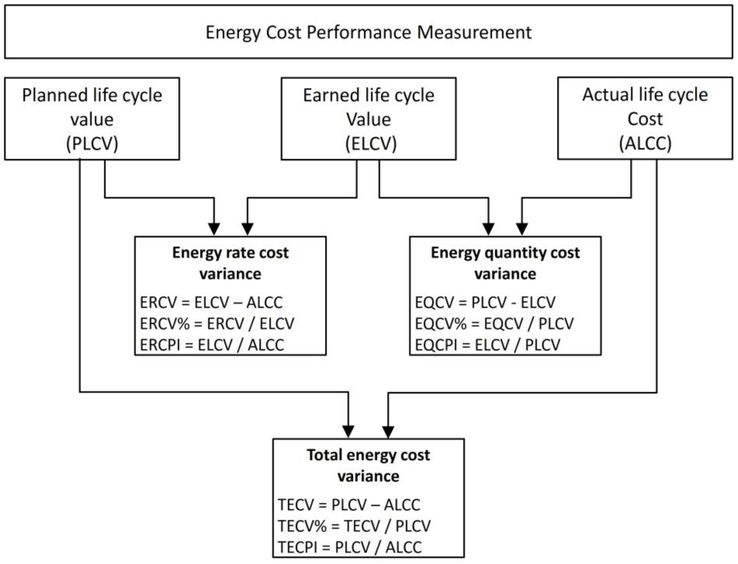
The ELCV was compared to the actual life cycle cost (ALCC) accrued up to the data date, the resultant cost variance (CV) is a cost performance metric quantifies the amount of cost deviation from the life cycle cost performance baseline of energy. Following the calculation procedure of the EVM, Equation (1) was applied to calculate the cost variance (CV) as follow:

CV = ELCV – ALCC = $124,640 − $142,746 = $−18,106

The negative variance implies that the actual energy cost is higher than its equivalent value in reference to the budgeted life cycle energy cost. However, this cost variance does not inform whether more or less energy has been consumed by the building; it quantifies the cost variance resulted from energy rate differences rather than consumed energy quantity in the building. This is because that the actual energy quantity is a common variable in both the ELCV and the actual life cycle cost (ALCC), and hence, the cost variance (CV) is determined based on energy rate variations rather than energy quantity. Consequently, since the cost variance (CV) only quantifies the cost deviation resulted from energy rate variations, it can be termed as energy rate cost variance, abbreviated ERCV.

The energy rate cost variance (ERCV) can be expressed as a percentage following Equation (2) by dividing the energy rate cost variance (ERCV) over the ELCV as follow:

ERCV% = (ERCV/ELCV) × 100 = ($−18,106/$124,640) × 100 = −14.53%

The energy rate cost variance percentage (ERCV%) corresponds to the cost variance percentage (CV%) used in the EVM. The ERCV% reports the percentage of the cost deviation from the budgeted value; it quantifies the magnitude of the cost saving or overrun resulted from energy rate variations. In the light of EVM, the above calculated ERCV% means that the energy cost is over budget by 14.53% since the result is negative.

Dividing the earned value over the actual cost yields the cost performance index (CPI) in a typical earned value analysis [22,35]. Similarly, dividing the ELCV by the actual life cycle cost (ALCC) of energy yields the energy rate cost performance index (ERCPI). The ERCPI is a measure of money spending efficiency, based on Equation (3), it can be calculated as follow:

ERCPI = ELCV/ALCC = $124,640/$142,746 = 0.87

The simple interpretation of the energy rate cost performance index (ERCPI) is that for each one dollar spent, only 0.87 dollar was earned. Keeping in mind that the cost deviation is resulted from energy rate variance, the ERCPI quantifies the magnitude of the cost deviation resulted from energy rate variations only.

Similar to the concept of comparing the earned value to the planned value in a typical earned value analysis which yields the schedule variance (SV) [22,24,25,26], comparing the ELCV with the planned life cycle value (PLCV) yields energy quantity cost variance (EQCV). The energy quantity cost variance (EQCV) is a modified term for the schedule variance (SV) proposed in the research to describe the difference between the ELCV and the planned life cycle value (PLCV). It can be calculated by adapting Equation (4) as follow:

EQCV = ELCV − PLCV = $124,640 − $432,438 = $−307,798

The energy quantity cost variance (EQCV) is different than the schedule variance (SV) which is used to determine whether the project is ahead or behind schedule in the EVM. For the case of energy, the energy quantity cost variance (EQCV) indicates whether less or more energy is being consumed in a building. This is because the ELCV is the product of multiplying the actual energy consumption by the baseline energy rates for the elapsed building operating years, and the planned life cycle value (PLCV) is determined by the baseline energy quantity and the baseline energy rates for the elapsed years as well. Consequently, the difference between the ELCV and the planned life cycle value (PLCV) represents the cost difference resulted from energy quantity variation rather than energy rates.

The energy quantity cost variance (EQCV) can be negative only in the case when less energy has been consumed than the baseline. This is because that for the EQCV to be negative, the ELCV should be less than the PLCV, and for this to happen, less actual energy should be consumed than the baseline. It is worth mentioning that the above calculations according to the earned value management approach yields a negative sign for a positive indicating variance, and hence, the sign of the variance has to be interpreted carefully. However, this issue can be resolved by adapting Equation (4) in reversed order as follow:

EQCV = PLCV − ELCV

Following Equation (5), the energy quantity cost variance (EQCV) can be expressed as a percentage as follow:

EQCV% = (EQCV/PLCV) × 100 = ($−307,798/$432,438) × 100 = −71.18%

This percentage is very close to the energy variance percentage which equals 71.07% which can be calculated as follow:

Building energy variance % = (Baseline energy consumption − Actual energy consumption)/Baseline energy consumption = (4,063,500 kWh − 1,175,772 kWh)/4,063,500 kWh = 71.07%

The energy quantity cost variance percentage (EQCV%) informs the percentage of energy saving or overrun but in term of monetary value. It can be inferred from the above EQCV% that around 71% of energy has been saved by the building since its commissioning compared to the baseline energy consumption.

Similar to the concept of the schedule performance index (SPI), following Equation (6), the energy quantity cost performance index (EQCPI) can be calculated as follow:

EQCPI = ELCV/PLCV = $124,640/$432,438 = 0.29

The energy quantity cost performance index (EQCPI) measures the efficiency of energy consumption in the building. The above calculated EQCPI for the case study means that for each day, month, or year, the building consumed 29% of the baseline energy calculated based on the monetary value.

The basic concept of the EVM is that comparing the planned cost with the actual cost can be misleading and does not allow for accurate cost performance measurement in projects [24,26]. However, it is found in the research that this not valid for the case of energy cost performance; comparing the planned life cycle value (PLCV) with the actual life cycle cost (ALCC) is still required to measure the overall cost performance of energy. This is because neither the ERCV nor the EQCV quantifies the overall cost variance resulted from actual energy consumption and actual energy rates. In the light of earned value approach, the total energy cost variance (TECV) can be calculated and reported as follow:

TECV = PLCV – ALCC = $432,438 − $142,746 = $289,692

The total energy cost variance (TECV) quantifies the cost deviation resulted from both energy consumption and rates variation. A positive variance implies cost saving while a negative variance indicates cost overrun. The shortcoming of the total energy cost variance (TECV) is that it does not inform whether the cost deviation is resulted from energy consumption or energy rate variations. Therefore, it should be used in conjunction with the ERCV and the EQCV to provide more detailed information about the causes of cost deviation.

The total energy cost variance (TECV) can be expressed as a percentage as follow:

Total energy cost variance percentage (TECV%) = TECV/PLCV × 100 = $289,692/$432,438 × 100 = 66.99%

This means that the total energy cost saving in the building is 66.99% compared to the baseline energy cost. The total energy cost performance index (TECPI) for the building can be calculated as follow:

TECPI = PLCV/ALCC = $432,438/$142,746 = 3.03

The total energy cost performance index (TECPI) quantifies the magnitude of the total cost saving or overrun. Similar to the concept of cost performance index (CPI) in the EVM, a value greater than 1.0 implies cost saving and vice versa. The above calculated TECPI means that for each one dollar spent on energy, a value of 3.03 dollars has been gained due to energy saving.

Table 5. Energy cost performance measurement using the earned value approach.

No.	Parameter	Value	Elapsed Building Operating Period
			2008	2009	2010	2011	2012	2013	2014
1	Baseline energy consumption (kWh)	Annual	580,500	580,500	580,500	580,500	580,500	580,500	580,500
		Cumulative	580,500	1,161,000	1,741,500	2,322,000	2,902,500	3,483,000	4,063,500
2	Planned life cycle value (PLCV) ($)	Annual	57,470	58,849	60,261	61,707	63,188	64,705	66,258
		Cumulative	57,470	116,319	176,580	238,287	301,475	366,180	432,438
3	Actual energy consumption (kWh)	Annual	243,900	151,284	140,160	127,068	165,960	175,224	172,176
		Cumulative	243,900	395,184	535,344	662,412	828,372	1,003,596	1,175,772
4	Actual energy cost ($)	Annual	29,611	18,367	17,016	15,427	20,149	21,273	20,903
		Cumulative	29,611	47,978	64,994	80,421	100,570	121,843	142,746
5	Planned energy rate ($/kWh)	Annual	0.099	0.101	0.104	0.106	0.109	0.111	0.114
6	Earned life cycle value (ELCV) ($)	Annual	24,146	15,280	14,577	13,469	18,090	19,450	19,628
		Cumulative	24,146	39,426	54,003	67,472	85,562	105,012	124,640
	Performance indicators and metrics
1	Energy rate cost variance
1.1	Energy rate cost variance (ERCV) ($)	Cumulative	−5465	−8,552	−10,991	−12,949	−15,008	−16,831	−18,106
1.2	Energy rate cost variance % (ERCV%)	Cumulative	−22.63%	−21.69%	−20.35%	−19.19%	−17.54%	−16.03%	−14.53%
1.3	Energy rate cost performance index (ERCPI)	Cumulative	0.820	0.820	0.830	0.840	0.850	0.860	0.870
2	Energy consumption cost variance
2.1	Energy quantity cost variance (EQCV) ($)	Cumulative	−33,324	−76,893	−122,577	−170,815	−215,913	−261,168	−307,798
2.2	Energy quantity cost variance % (EQCV%)	Cumulative	−57.99%	−66.11%	−69.42%	−71.68%	−71.62%	−71.32%	−71.18%
2.3	Energy quantity cost performance index (EQCPI)	Cumulative	0.42	0.34	0.31	0.28	0.28	0.29	0.29
3	Total energy cost variance
3.1	Total energy cost variance (TECV) ($)	Cumulative	27,859	68,341	111,586	157,866	200,905	244,337	289,692
3.2	Total energy cost variance percentage (TECV%)	Cumulative	48.48%	58.75%	63.19%	66.25%	66.64%	66.73%	66.99%
3.3	Total energy cost performance index (TECPI)	Cumulative	1.94	2.42	2.72	2.96	3.00	3.01	3.03

shows annual analysis for energy cost performance using the earned value approach. The earned value calculations for energy cost performance indicators and metrics are summarized in Figure 6.

6. Conclusions

In this research, the EVM was examined to measure the actual life cycle cost performance of energy in green buildings. With slight methodological and terminological adaptations, it is found that the EVM approach is applicable and meaningful in measuring the actual energy cost performance in green buildings. The ELCV of energy is the value of the consumed energy in reference to the total estimated life cycle budget of energy. It can be determined by multiplying the actual energy consumption in each building operating year by the baseline energy rate for the corresponding year.

The key finding in this research is that using the EVM approach to measure the actual energy cost performance allows an exhaustive cost impact analysis of energy performance gap. The traditional cost performance measurement which compares the actual energy cost with the baseline costs shows that the total energy cost saving in the case study is around 66.99% compared to the industry baseline. While the earned value analysis reveals that the energy cost saving is around 71.18% compared to the baseline, and this is because the earned value approach allows isolating the impact of energy price increase on the energy cost performance of the building.

The significance of the earned value approach is that it allows for quantifying the cost variance which results from actual energy rates differences in isolation from the cost variance which results from energy consumption variations than the energy consumption baseline. This allows green building owners to fairly evaluate the actual economic performance of their green buildings, since using the earned value approach they can isolate the effect of energy price fluctuations on the actual energy cost performance of their green facilities.

It is also found that using the EVM approach does not eliminate the need to compare the actual energy cost with the baseline cost; comparing the actual cost against the planned cost is still recommended to measure the total energy cost variance which results from actual energy consumption and rates variations than the baseline.

This research presents a novel approach to measure the actual energy cost performance of green buildings. It is the first research that examines the earned value management (EMV) within the context of buildings life cycle cost. Although the used case study in the research is a typical green building, further research is required to replicate the findings and to investigate how the earned value performance indicators can be used to forecast future energy cost performance in green buildings. Future research is also recommended to examine using the EVM to measure the actual life cycle cost performance of other performance areas in green buildings.

References

1. United Nations Environment Programme. Towards a Green Economy: Pathways to Sustainable Development and Poverty Eradication; United Nations Environment Programme (UNEP), 2011; Available online: http://www.unep.org/greeneconomy/Portals/88/documents/ger/9.0_Buildings.pdf (accessed on 7 April 2014).
2. Kats, G.; Alevantis, L.; Berman, A.; Mills, E.; Perlman, J. The Costs and Financial Benefits of Green Buildings. A Report to California’s Sustainable Building Task Force; U.S. Green Building Council, 2003; Available online: http://www.usgbc.org/Docs/News/News477.pdf (accessed on 4 April 2014).
3. Yudelson, J. The Green Building Revolution; Island Press: Washington, DC, USA, 2008. [Google Scholar]
4. Kibert, C.J. Sustainable Construction: Green Building Design and Delivery, 3rd ed.; John Wiley & Sons Inc.: Hoboken, NJ, USA, 2012. [Google Scholar]
5. Yudelson, J. Green Building A to Z: Understanding the Language of Green Building; New Society Publishers: Gabriola Islands, BC, Canada, 2007. [Google Scholar]
6. Ries, R.; Bilec, M.M.; Needy, K.L.; Gokhan, N.M. The Economic Benefits of Green Buildings: A Comprehensive Case Study. Eng. Econ. 2006, 51, 259–295. [Google Scholar] [CrossRef]
7. GSA Public Buildings Service. Assessing Building Performance: A Post Occupancy Evaluation of 12 GSA Buildings Research; GSA Public Buildings Service, 2008. Available online: http://www.gsa.gov/graphics/pbs/GSA_AssessGreen_white_paper.pdf (accessed on 29 March 2014).
8. Kats, G. Green Building Costs and Financial Benefits; Massachusetts Technology Collaborative: Boston, MA, USA, 2003. [Google Scholar]
9. Kats, G. Greening Our Built World: Costs, Benefits, and Strategies; Island Press: Washington, DC, USA, 2010. [Google Scholar]
10. Torcellini, P.; Pless, S.; Deru, M.; Griffith, B.; Long, N.; Judkoff, R. Lessons Learned from Case Studies of Six High-Performance Buildings; Technical Report NREL/TP-550-37542; National Renewable Energy Laboratory (NREL): Golden, CO, USA, 2006. Available online: http://www.nrel.gov/docs/fy06osti/37542.pdf (accessed on 17 February 2014).
11. Menezes, A.C.; Cripps, A.; Bouchlaghem, D.; Buswell, R. Predicted vs. actual energy performance of non-domestic buildings: Using post-occupancy evaluation data to reduce the performance gap. Appl. Energy 2012, 97, 355–364. [Google Scholar] [CrossRef] [Green Version]
12. De Wilde, P. The gap between predicted and measured energy performance of buildings: A framework for investigation. Autom. Constr. 2014, 41, 40–49. [Google Scholar] [CrossRef]
13. USGBC Research Committee. A National Green Building Research Agenda; U.S. Green Building Council, 2008; Available online: http://www.usgbc.org/Docs/Archive/General/Docs3402.pdf (accessed on 15 March 2014).
14. Burnett, J. Costs and Benefits of Building Commissioning. Hong Kong Inst. Eng. Trans. 2008, 15, 9–16. [Google Scholar]
15. Cohen, R.; Standeven, M.; Bordass, B.; Leaman, A. Assessing building performance in use 1: The Probe process. Build. Res. Inf. 2001, 29, 85–102. [Google Scholar] [CrossRef]
16. Bordass, B.; Cohen, R.; Standeven, M.; Leaman, A. Assessing Building Performance in Use 3: Energy Performance of the Probe Buildings. Build. Res. Inf. 2001, 29, 114–128. [Google Scholar] [CrossRef]
17. Salehi, M.M.; Terim Cavka, B.; Frisque, A.; Whitehead, D.; Bushe, W.K. A Case Study: The Energy Performance Gap of the Center for Interactive Research on Sustainability at the University of British Columbia. J. Build. Eng. 2015, 4, 127–139. [Google Scholar] [CrossRef]
18. Norford, L.K.; Socolow, R.H.; Hsieh, E.S.; Spadaro, G.V. Two-to-One Discrepancy Between Measured and Predicted Performance of a “Low-Energy” Office Building: Insights from a Reconciliation Based on the DOE-2 Model. Energy Build. 1994, 21, 121–131. [Google Scholar] [CrossRef]
19. Turner, C.; Frankel, M. Energy Performance of LEED for New Construction Buildings (Final Report); U.S. Green Building Council: Washington, DC, USA, 2008; Available online: http://www.usgbc.org/Docs/Archive/General/Docs3930.pdf (accessed on 14 July 2014).
20. GSA Public Buildings Service. Green Building Performance: A Post Occupancy Evaluation of 22 GSA Buildings; GSA Public Buildings Service: Washington, DC, USA, 2011. Available online: http://www.gsa.gov/graphics/pbs/Green_Building_Performance.pdf (accessed on 24 April 2014).
21. Fowler, K.M.; Rauch, E.M. Assesing Green building performance: A Post Occupancy Evaluation of 12 GSA Buildings; Pacific Northwest National Laboratory: Washington, DC, USA, 2008. [Google Scholar]
22. Project Management Institute. Practice Standard for Earned Value Management, 2nd ed.; Project Management Institute, Inc.: Pennsylvania, PA, USA, 2011. [Google Scholar]
23. Song, L. Earned Value Management: A Global and Cross-Industry Perspective on Current EVM Practice. Proj. Manag. J. 2010, 41, 90. [Google Scholar] [CrossRef]
24. Fleming, Q.W.; Koppelman, J.M. Earned Value Project Management, 2nd ed.; Project Management Institute, Inc.: Pennsylvania, PA, USA, 2000. [Google Scholar]
25. Hinze, J.W. Construction Planning and Scheduling, 4th ed.; Pearson Prentice Hall: Upper Saddle River, NJ, USA, 2011. [Google Scholar]
26. Mubarak, S. Construction Project Scheduling and Control, 2nd ed.; John Wiley & Sons, Inc.: Hoboken, NJ, USA, 2010. [Google Scholar]
27. Yudelson, J. Marketing Green Building Services: Strategies for Success, 1st ed.; Elsevier Ltd.: Beijing, China, 2008. [Google Scholar]
28. Levine, M.; Ürge-Vorsatz, D.; Blok, K.; Geng, L.; Harvey, D.; Lang, S.; Levermore, G.; Mongameli, A.; Mirasgedis, S.; Novikova, A.; et al. Residential and commercial buildings. In Climate Change 2007: Mitigation. Contribution of Working Group III to the Fourth Assessment Report of the Intergovernmental Panel on Climate Change; Metz, B., Davidson, O.R., Bosch, P.R., Dave, R., Meyer, L.A., Eds.; Cambridge University Press: Cambridge, UK; New York, NY, USA, 2007; pp. 388–446. [Google Scholar]
29. Laustsen, J. Energy Efficiency Requirements in Building Codes, Energy Efficiency Policies for New Buildings; International Energy Agency (IEA): Paris, France, 2008; Available online: http://www.iea.org/publications/freepublications/publication/Building_Codes.pdf (accessed on 7 April 2014).
30. Sadineni, S.B.; Madala, S.; Boehm, R.F. Passive building energy savings: A review of building envelope components. Renew. Sustain. Energy Rev. 2011, 15, 3617–3631. [Google Scholar] [CrossRef]
31. Leipziger, D. Comparing Building Energy Performance Measurement. A Framework for International Energy Efficiency Assessment Systems; Institute for Market Transformation (IMT): Washington, DC, USA, 2013. [Google Scholar]
32. Popescu, C.M.; Charoenngam, C. Project Planning, Scheduling, and Control in Construction: An Encyclopedia of Terms and Applications; John Wiley & Sons: New York, NY, USA, 1995. [Google Scholar]
33. Fleming, B.Q.W.; Koppelman, J.M. The Two Most Useful Earned Value Metrics: The CPI and the TCPI. PM World Today 2009, 11, 1–9. [Google Scholar]
34. Project Management Institute. Practice Standard for Earned Value Management; Project Management Institute, Inc.: Pennsylvania, PA, USA, 2005. [Google Scholar]
35. American National Standards Institute. Earned Value Management Systems (ANSI/EIA-748-B-2007); Government Electronics and Information Technology Association, Standards & Technology Department: Arlington, VA, USA, 2007. [Google Scholar]
36. Kwak, Y.H.; Sciences, D.; George, T. History, Practices, and Future of Earned Value Management in Government: Perspectives from NASA. Proj. Manag. J. 2012, 43, 77–90. [Google Scholar] [CrossRef]
37. Fleming, Q.; Koppelman, J. Earned Value Lite: Earned Value for the Masses. 2007. Available online: http://www.oracle.com/us/products/applications/042745 (accessed on 6 March 2016).
38. Yin, R.K. Case Study Research Design & Methods, 4th ed.; SAGE Publications, Inc.: Thousand Oaks, CA, USA, 2009. [Google Scholar]
39. Saunders, M.; Lewis, P.; Thornhill, A. Research Methods for Business Students, 5th ed.; Prentice Hall: Lombarda, Italy, 2009. [Google Scholar]
40. Swanborn, P. Case Study Research: What, Why and How? SAGE Publications Ltd.: New Delhi, India, 2010. [Google Scholar]
41. Gerring, J. What Is a Case Study and What Is It Good for? Am. Political Sci. Rev. 2004, 98, 341–354. [Google Scholar] [CrossRef]
42. Eisenhardt, K.M. Building Theories from Case Study Research. Acad. Manag. Rev. 1989, 14, 532–550. [Google Scholar] [CrossRef]
43. Fellows, R.; Liu, A. Research Methods for Construction, 3rd ed.; Wiley-Blackwell Publishing Ltd.: Chichester, UK, 2008. [Google Scholar]
44. Weiss, N.A. Elementary Statistics, 8th ed.; Pearson: Boston, MA, USA, 2012. [Google Scholar]
45. Hancock, D.; Algozzine, B. Doing Case Study Research: A Practical Guide for Beginning Researchers; Teachers College Press: New York, NY, USA, 2006. [Google Scholar]
46. Yin, R.K. Case Study Research: Design and Methods, 3rd ed.; SAGE Publications, Inc.: Thousand Oaks, CA, USA, 2003. [Google Scholar]
47. Flyvbjerg, B. Five Misunderstandings About Case-Study Research. Qual. Inq. 2006, 12, 219–245. [Google Scholar] [CrossRef]
48. Seawright, J.; Gerring, J. Case Selection Techniques in Case Study Research: A Menu of Qualitative and Quantitative Options. Political Res. Q. 2008, 61, 294–308. [Google Scholar] [CrossRef]
49. Georgia Bureau of Investigation. GBI Certified Buildings. Available online: http://www.greenbuildingindex.org/ (accessed on 18 May 2015).
50. Malaysian Green Technology Corporation. GEO Building Performance. Available online: http://www.greentechmalaysia.my (accessed on 6 September 2015).
51. Shafii, F. Status of Sustainable Building in South-East Asia; International Initiative for a Sustainable Built Environment, 2007; Available online: http://www.iisbe.org/sbconferences/Malaysia_SB_Report_SB08.pdf (accessed on 14 May 2015).
52. Aun, A.C. Green Building Index—MS1525: Applying MS1525:2007 Code of Practice on Energy Efficiency and Use of Renewable Energy for Non-Residential Buildings; Green Building Index, 2009; Available online: http://www.greenbuildingindex.org/Resources/20090214-GBI MS1525-2007 Seminar/20090214-GBI MS1525-2007 Seminar (CSA) Notes.pdf (accessed on 14 May 2015).
53. Abu Bakar, N.N.; Hassan, M.Y.; Abdullah, H.; Rahman, H.A.; Abdullah, M.P.; Hussin, F.; Bandi, M. Energy Efficiency Index as an Indicator for Measuring Building Energy Performance: A Review. Renew. Sustain. Energy Rev. 2015, 44, 1–11. [Google Scholar] [CrossRef]
54. Central Bank of Malaysia. Rates and Statistics. Available online: http://www.bnm.gov.my/index.php?ch=statistic&pg=stats_exchangerates (accessed on 26 May 2015).
55. Kirk, S.J.; Dell’isola, A.J. Life Cycle Costing for Design Professionals, 2nd ed.; McGraw-Hill, Inc.: New York, NY, USA, 1995. [Google Scholar]
56. Flanagan, R.; Jewell, C.; Norman, G. Whole Life Appraisal for Construction; Blackwell Publishing Ltd.: Oxford, UK, 2005. [Google Scholar]
57. International Organization for Standardization. Buildings and Constructed Assets—Service-Life Planning—Part 5: Life-Cycle Costing (ISO 15686-5:2008), 1st ed.; International Organization for Standardization: Geneva, Switzerland, 2008. [Google Scholar]
58. International Organization for Standardization. Buildings and Constructed Assets—Service Life Planning—Part 1: General Principles/Framework (ISO 15686-1:2008), version 2.2; International Organization of Standardization: Geneva, Switzerland, 2008. [Google Scholar]
59. Kelly, D. Design Life of Buildings: A Scoping Study; Scottish Building Standards Agency: Livingston, UK, 2007; Available online: http://www.gov.scot/resource/doc/217736/0091011.pdf (accessed on 23 April 2014).
60. Hock, B.; Roden, L. Financial Reporting, Planning, Performance, and Control: Part 1, 6th ed.; Hock International, LLC: Columbus, OH, USA, 2014; Volume 1. [Google Scholar]
61. Department of Statistics Malaysia. Malaysia Economic Statistics—Time Series Report 2015; Department of Statistics Malaysia, 2015. Available online: https://www.statistics.gov.my/dosm/uploads/files/3_Time Series/Malaysia Time Series 2013/Penerbitan_Time_Series_2013.pdf (accessed on 15 May 2015).
62. Blank, L.; Tarquin, A. Engineering Economy, 7th ed.; McGraw-Hill, Inc.: New York, NY, USA, 2012. [Google Scholar]
63. Fowler, K.; Rauch, E.; Henderson, J.; Kora, A. Re-Assessing Green Building Performance: A Post Occupancy Evaluation of 22 GSA Buildings; Pacific Northwest National Laboratory: Richland, WA, USA, 2011. Available online: http://www.pnl.gov/main/publications/external/technical_reports/PNNL-19369.pdf (accessed on 27 August 2014).
64. United Nations Environment Programme. Building Sector Energy Effeciency Project (BSEEP); United Nations Environment Programme (UNEP), 2015; Available online: http://www.my.undp.org/content/dam/malaysia/docs/Building Sector Energy Efficiency Projects Prodoc.pdf (accessed on 16 April 2015).
65. Energy Commission. The Energy Commission Diamond Building. Available online: http://www.st.gov.my/index.php/ms/about-us2/energy-commission-diamond-building.html (accessed on 5 June 2015).
66. Moghimi, S.; Azizpour, F.; Mat, S.; Lim, C.H.; Salleh, E.; Sopian, K. Building Energy Index and End-use Energy Analysis in Large-scale Hospitals-Case Study in Malaysia. Energy Effic. 2014, 7, 243–256. [Google Scholar] [CrossRef]
67. Saidur, R. Energy Consumption, Energy Savings, and Emission Analysis in Malaysian Office Buildings. Energy Policy 2009, 37, 4104–4113. [Google Scholar] [CrossRef]
68. Energy Commission. Electricity Supply Industry in Malaysia—Report of Performance and Statistical Information 2007; Energy Commission: Kuala Lumpur, Malaysia, 2007. Available online: http://www.st.gov.my/index.php/industry/statistics-reports.html (accessed on 6 September 2015).
Figure 1. Graphic representation of earned value management (EVM), adopted from PMI [22].
Energies 09 00188 g001
Figure 2. GEO Building, general view, from Malaysian Green Technology Corporation [50].
Energies 09 00188 g002
Figure 3. Building energy performance compared to industry baseline.
Energies 09 00188 g003
Figure 4. Graphic representation of energy life cycle cost baseline.
Energies 09 00188 g004
Figure 5. Energy cost performance measurement parameters.
Energies 09 00188 g005
Figure 6. Actual energy cost performance indicators and metrics calculations using the earned value approach.
Energies 09 00188 g006