Electric Vehicle Charging and Discharging Coordination on Distribution Network Using Multi-Objective Particle Swarm Optimization and Fuzzy Decision Making

Abstract

This paper proposed a optimal strategy for coordinated operation of electric vehicles (EVs) charging and discharging with wind-thermal system. By aggregating a large number of EVs, the huge total battery capacity is sufficient to stabilize the disturbance of the transmission grid. Hence, a dynamic environmental dispatch model which coordinates a cluster of charging and discharging controllable EV units with wind farms and thermal plants is proposed. A multi-objective particle swarm optimization (MOPSO) algorithm and a fuzzy decision maker are put forward for the simultaneous optimization of grid operating cost, CO₂ emissions, wind curtailment, and EV users’ cost. Simulations are done in a 30 node system containing three traditional thermal plants, two carbon capture and storage (CCS) thermal plants, two wind farms, and six EV aggregations. Contrast of strategies under different EV charging/discharging price is also discussed. The results are presented to prove the effectiveness of the proposed strategy.

1. Introduction

Electric vehicles (EVs) will play a vital role in the future’s sustainable transportation systems, since this technology is promising for environment, energy security, and improved fuel economy. Certain issues will need to be addressed in the event that the number of EVs on the road increases. One vital issue is the method by which these vehicles will be charged and if today’s grid can sustain the increased demand due to more EVs. Although EVs’ growing energy demand seems to be a heavy burden to the power gird, they can actually benefit the grid if we control the charging and discharging behavior of them properly. For example, nowadays, a growing quantity of renewable energy, such as wind and solar generation, is connected to the grid [1]. Due to the discontinuity of the renewable energy power generation, an energy storage system is needed to assist the grid to absorb the volatility of renewable energy power. Electric vehicles are considered to be the energy storage device with the most potential to absorb the volatility of renewable energy [2]. When a large number of EVs are aggregated, the huge total battery capacity is sufficient to stabilize the disturbance of the grid caused by the distributed power grid interconnection [3].

In earlier research, Amory Lovins first proposed the concept “V2G” in 1995, which is an abbreviation of “vehicle to grid”, meaning EVs serve in discharge mode to support the grid. This concept was well explained and developed later by William Kempton of Delaware University [4,5,6,7]. In the recent literature, a number of studies have been conducted on V2G. It has been shown that EVs can be dispatched to follow power system regulation signals [8,9]. Literature [10,11] has studied the integration of EVs in a regional wind-thermal system; other works [12,13] proposed coordinated strategies for EV and renewable sources considering cost and emission reductions, and others [14,15,16,17] have proposed optimal scheduling strategies for V2G. These studies, however, did not consider the EV user’s cost while doing optimization of such a V2G system. Since deep charging and discharging will greatly affect the life of EV’s battery [2], if only the cost of grid is taken into consideration while the cost to EV users is neglected while conducting the calculation, the results might be unrealistic and unacceptable for EV users.

In today’s power system, while wind turbines, thermal plants, and EVs are all integrated into the grid, ramp rates, reserve capacity, fossil costs, carbon emissions, environmental costs, carbon capture costs, and power balance should all be considered when developing an optimal coordination strategy [13]. From the viewpoint of transmission grid, it is a quite complicated problem. Consequently, from the viewpoint of multi-objective optimization, the complicated optimal coordination problem can be formulated as a multi-objective problem (MOP) [18], which is solved by using a proposed multi-objective particle swarm optimization algorithm (MOPSO) [19,20]. Furthermore, to extract the best compromise solution from the Pareto optimal solution set, the fuzzy optimality decision making (FODM) method [21,22,23,24] is proposed in this paper.

One of the main contributions of this paper is the presentation of a dynamic environmental dispatch model which coordinates a cluster of charging and discharging controllable EV units with large-scale wind power farms and large thermal plants. A MOPSO algorithm for the simultaneous optimization of grid operating costs, CO₂ emissions, wind curtailment, and EV user’s cost is presented. With this heuristic, evolutionary algorithm, a set of Pareto optimal solution of the MOP is obtained. As another contribution, the FODM method is proposed to extract out the best compromise solution from the Pareto optimal set. With this approach, the objective function value weighting factors are processed with fuzzy members. A fuzzy decision, which can be viewed as an intersection of the given goals, is made. This process is much like the way we human beings does when we are making decisions [21].

The rest of this paper is structured as follows. In Section 2, the concept and mathematical model of the thermal-wind-EV system is discussed. In Section 3, the multi-objective optimization problem of grid operating costs, CO₂ emissions, and wind curtailment is formulated. In Section 4, the MOPSO algorithm and the FODM method is introduced, and the process of the algorithm is described in detail. Section 5 provides a simulation case study, and discusses the results. Finally, the conclusion is stated in Section 6.

2. System Description and Models

2.1. System Concept

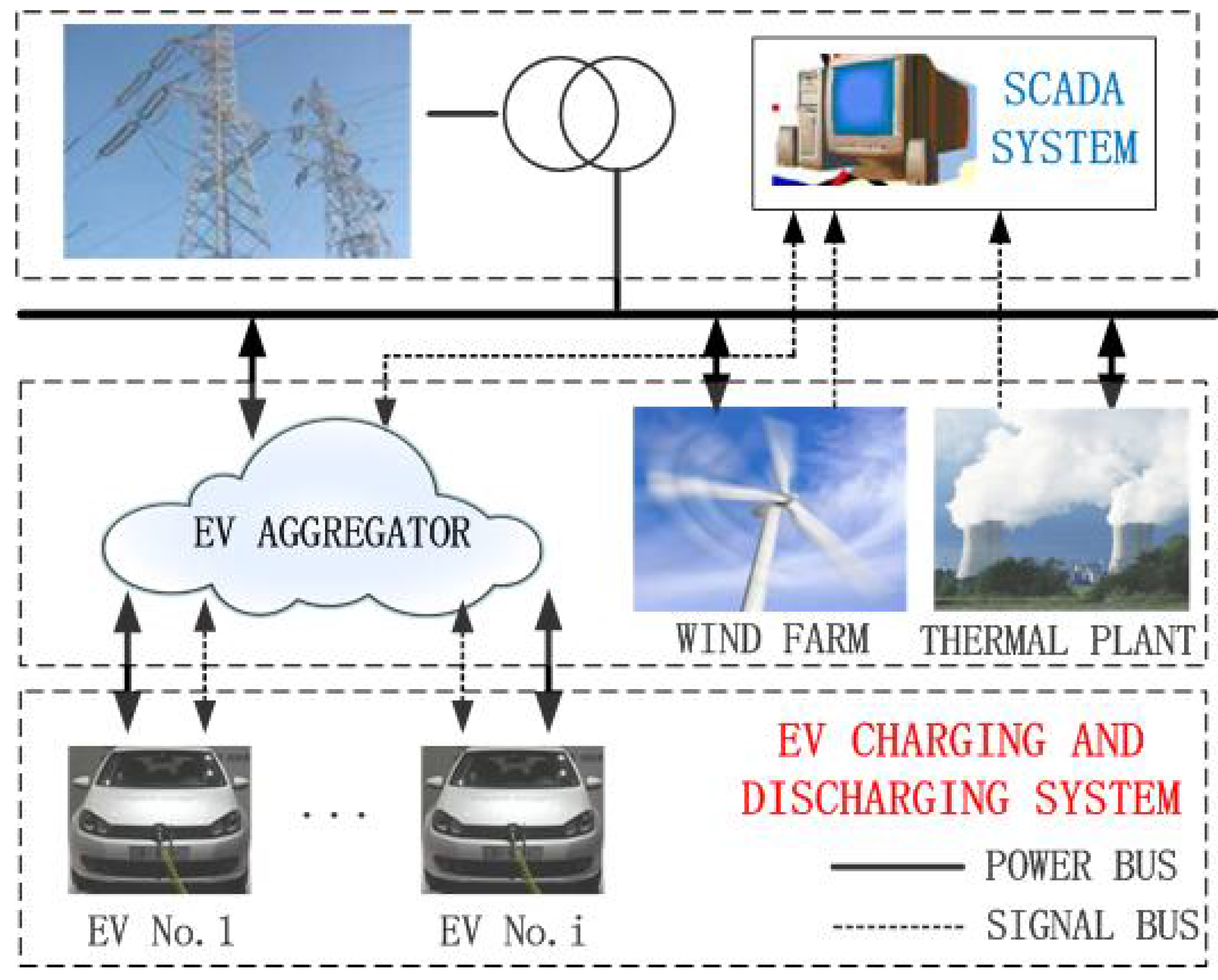
In order to better schedule the charging and discharging behavior of EVs, since the capacity of a single EV’s battery is hard to have a measurable influence on the transmission grid. The concept “EV aggregator” is present in this paper to represent a number of grid-connected controllable EVs. By aggregating EVs, a conceptual framework for a thermal-wind-EV system is built up as in Figure 1 shows:

In this conceptual system, at the top layer, the supervisory control and data acquisition system (SCADA) system is used for a double purpose: one is to collect information, such as EV battery status, EV number, predicted wind power, predicted load, etc., which are feedback from EV aggregator, wind farms, and thermal plants; another is to make a schedule for the above units to generate/absorb power to/from the transmission grid.

At the middle layer, wind farms, thermal plants, and EV aggregator receive a working schedule transferred from the top layer and make a detailed work plan for each wind turbine, thermal power generating unit, and EV unit inside the system. The middle layer then send out power instructions to dispatch the input or output power of the aforementioned power units.

At the bottom layer, while a large number of EVs are connected to the transmission grid via power electronics devices, Each EV unit follows the power instruction from the middle layer and feeds its current status back constantly to the aggregator so that the system is able to adjust its power distribution strategy according to the real-time model.

2.2. Electric Vehicles Aggregator Model

The electric quantity equation of EV i is given as follows:

$$E_{i,k}=(1-d_{\mathrm{b}})E_{i,k-1}+\left({\mathsf{\eta }}_{\mathrm{C}}{P}_{i,k}^{\mathrm{C}}-\frac{P_{i,k}^{\mathrm{D}}}{{\mathsf{\eta }}_{\mathrm{D}}}\right)\Delta t$$

(1)

where $E_{i,k}$ is the electric quantity of EV i at the time period k. $d_{\mathrm{b}}$ is battery self-discharge rate, ${\mathsf{\eta }}_{\mathrm{C}}$ and ${\mathsf{\eta }}_{\mathrm{D}}$ are the battery charging and discharging efficiency factor, respectively, while $P_{i,k}^{\mathrm{C}}$ and $P_{i,k}^{\mathrm{D}}$ are the charging and discharging power of EV i at time period k, respectively. $\Delta t$ is the time step, given in hour.

The cost equation of the EV aggregator is as follows:

$$G_{\mathrm{C},i}^k\left(P_{i,k}^{\mathrm{C}}\right)={\mathsf{\gamma }}_{i,k}^{\mathrm{C}}·P_{i,k}^{\mathrm{C}}$$

(2)

$$G_{\mathrm{D},i}^k\left(P_{i,k}^{\mathrm{D}}\right)={\mathsf{\gamma }}_{i,k}^{\mathrm{D}}·P_{i,k}^{\mathrm{D}}$$

(3)

where ${\mathsf{\gamma }}_{i,k}^{\mathrm{C}}$ is the EV’s charging price, while ${\mathsf{\gamma }}_{i,k}^{\mathrm{D}}$ is the discharging cost for V2G services.

Equations (1)–(3) are subject to constraints as follows:

(1) Power constraints.

$$P_{i,k}^{\left(\mathrm{C},\text{min}\right)}\le P_{i,k}^{\mathrm{C}}\le P_{i,k}^{\left(\mathrm{C},\text{max}\right)}$$

(4)

$$P_{i,k}^{\left(\mathrm{D},\text{min}\right)}\le P_{i,k}^{\mathrm{D}}\le P_{i,k}^{\left(\mathrm{D},\text{max}\right)}$$

(5)

where $P_{i,k}^{\left(\mathrm{C},\text{min}\right)}$ and $P_{i,k}^{\left(\mathrm{C},\text{max}\right)}$ are the lower and upper limits of EV’s charging power $P_{i,k}^{\mathrm{C}}$ respectively, $P_{i,k}^{\left(\mathrm{D},\text{min}\right)}$ and $P_{i,k}^{\left(\mathrm{D},\text{max}\right)}$ are the lower and upper limits of EV’s discharging power $P_{i,k}^{\mathrm{D}}$, respectively.

(2) Electric quantity constraints.

$$E_{i,k}^{\text{min}}\le E_{i,k}\le E_{i,k}^{\text{max}}$$

(6)

$E_{i,k}^{\text{min}}$ and $E_{i,k}^{\text{max}}$ are the lower and upper limits of $E_{i,k}$, which are decided by EV’s battery capacity B and its depth of discharge (DoD):

$$E_{i,k}^{\text{min}}=(1-\text{DoD})·B$$

(7)

$$E_{i,k}^{\text{max}}=B$$

(8)

(3) EV will not charge and discharge at the same time period.

$$\left\{\begin{array}{c}{P}_{i,k}^{\mathrm{C}}=\mathsf{\kappa }·P_{i,k}^{\mathrm{C}}\hfill \\ P_{i,k}^{\mathrm{D}}=(1-\mathsf{\kappa })·P_{i,k}^{\mathrm{D}}\hfill \end{array}\right.$$

(9)

$$\mathsf{\kappa }=\left\{\begin{array}{cc}1\hfill & \hfill SO{C}_{i,k}-SO{C}_{i,\mathrm{dmin}}^{\mathrm{D}}<0orSO{C}_{i,\mathrm{cmax}}^{\mathrm{C}}-SO{C}_{i,k}>0\\ 0\hfill & \hfill \text{else}\end{array}\right.$$

(10)

where $SO{C}_{i,k}$ is the battery state of charge of $E{V}_i$ , which is decided by the equation:

$$SO{C}_{i,k}=\frac{E_{i,k}}{E_{i,k}^{\text{max}}}\times 100\%$$

(11)

$SO{C}_{i,\mathrm{d}\hspace{0.17em}\text{min}}^{\mathrm{D}}$ is the lower bound of state of charge (SOC) when EV is discharging, while $SO{C}_{i,\mathrm{c}\hspace{0.17em}\text{max}}^{\mathrm{C}}$ is the upper bound of SOC when EV is charging. These bounds are set by EV users.

2.3. Thermal Plant Model

In this thermal plant model, we consider two kinds of thermal generating plants, including traditional coal-fired (TC) power plants and coal-fired power plants with carbon capture and storage (CCS). The consumption function of traditional coal-fired power plants can be approximated by quadratic function:

$$F_i^{\mathrm{U}}=a_i\left(P_{i,k}^{\mathrm{U}}\right)+b_i{P}_{i,k}^{\mathrm{U}}+c_i$$

(12)

where $P_{i,k}^{\mathrm{U}}$ is the active power output of TC power plant i at time period k, while $a_i$, $b_i$, and $c_i$ are consumption characteristic factors of the function.

The emission equation of traditional coal-fired power plant is as follow:

$$C_i^{\mathrm{U}}={\mathsf{\alpha }}_i\left(P_{i,k}^{\mathrm{U}}\right)+{\mathsf{\beta }}_i$$

(13)

where ${\mathsf{\alpha }}_i$ and ${\mathsf{\beta }}_i$ are emission characteristic factors of the function.

CCS power plants need to consume a large amount of energy to capture CO₂, which leads to an increase in generating cost. Assuming that the capture rate of CO₂ is ω, then the consumption function $F_i^{\mathrm{C}}$ and emission function $C_i^{\mathrm{C}}$ of CCS power plants are as follows:

$$F_i^{\mathrm{C}}=a_i\left(P_{i,k}^{\text{ccs}}\right)+b_i{P}_{i,k}^{\text{ccs}}+c_i$$

(14)

$$C_i^{\mathrm{C}}=\left(1-\mathsf{\omega }\right)\left[{\mathsf{\alpha }}_i\left(P_{i,k}^{\text{ccs}}\right)+{\mathsf{\beta }}_i\right]$$

(15)

where $P_{i,k}^{\text{ccs}}$ is the active power output of CCS power plant i at time period k.

The amount of captured CO₂ is calculated as follows:

$$C_i^{\text{ca}}=\mathsf{\omega }·\left[{\mathsf{\alpha }}_i\left(P_{i,k}^{\text{ccs}}\right)+{\mathsf{\beta }}_i\right]$$

(16)

Equations (12) – (16) are subject to constraints as follows:

(1) Power constraints

$$P_{i,k}^{\left(\mathrm{U},\text{min}\right)}\le P_{i,k}^{\mathrm{U}}\le P_{i,k}^{\left(\mathrm{U},\text{max}\right)}$$

(17)

$$P_{i,k}^{\left(\text{ccs},\text{min}\right)}\le P_{i,k}^{\text{ccs}}\le P_{i,k}^{\left(\text{ccs},\text{max}\right)}$$

(18)

where $P_{i,k}^{\left(\mathrm{U},\text{min}\right)}$ and $P_{i,k}^{\left(\mathrm{U},\text{max}\right)}$ are the lower and upper limits of TC plant power output $P_{i,k}^{\mathrm{U}}$, $P_{i,k}^{\left(\text{ccs},\text{min}\right)}$ and $P_{i,k}^{\left(\text{ccs},\text{max}\right)}$ are the lower and upper limits of CCS plant power output $P_{i,k}^{\text{ccs}}$.

(2) Ramping rate constraints

For the safety of thermal plant operation, the power output of TC plants and CCS plants must be subject to ramping rate constraints as follows:

$$\begin{array}{c}\hfill \left\{\begin{array}{c}{P}_{i,k}^{\mathrm{U}/\text{ccs}}-P_{i,k-1}^{\mathrm{U}/\text{ccs}}\le U_{\mathrm{G}}\\ P_{i,k-1}^{\mathrm{U}/\text{ccs}}-P_{i,k}^{\mathrm{U}/\text{ccs}}\le D_{\mathrm{G}}\end{array}\right.\end{array}$$

(19)

where $U_{\mathrm{G}}$ and $D_{\mathrm{G}}$ are the highest increase and decrease value of the generating unit power output between adjacent time period.

2.4. Wind Farm Model

When wind power generation is allowed to be integrated into the grid, the power output of thermal plants decreased if the wind power generation increases. Assuming that the upper bound of wind generation is equal to the negative peak load regulation ability of thermal plants [25]:

$$P_{\text{max}}^k=P_{\mathrm{L}}^k+{\displaystyle \sum _{i=1}^{N_{\mathrm{v}}}}\left(P_{i,k}^{\mathrm{C}}-P_{i,k}^{\mathrm{D}}\right)-{\displaystyle \sum _{i=1}^N}{P}_{\text{min},i}^k$$

(20)

where $P_{\text{min},i}^k$ is the lower limit of thermal generating units, which includes TC and CCS units; $P_{\mathrm{L}}^k$ is the system load; $P_{\text{loss}}^k$ is the system loss; $P_{i,k}^{\mathrm{C}}$ and $P_{i,k}^{\mathrm{D}}$ are $E{V}_i$’s charging and discharging power, respectively.

Consequently, the generating capacity of wind farm i at time period k can be calculated as follows:

$$P_{\text{wa},i}^k=\text{min}\left(P_{\text{wc},i}^k,\frac{P_{\text{wr},i}}{{\displaystyle \sum _{i=1}^{Nw}}{P}_{\text{wr},i}}{P}_{\text{max}}^k\right)$$

(21)

where $P_{\text{wa},i}^k$ is the available generating capacity, $P_{\text{wc},i}^k$ is the forecasted wind generation capacity, and $P_{\text{wr},i}$ is the rated capacity that of Wind farm i.

The cost function of wind farms is as follows:

$$W_i^k\left(P_{\mathrm{w},i}^k\right)={\epsilon }_i·P_{\mathrm{w},i}^k$$

(22)

where ${\epsilon }_i$ is the operating cost factor of wind farms.

Equations (20) – (22) are subject to constraint as follows:

$$0\le P_{\mathrm{w},i}^k\le P_{\text{wa},i}^k$$

(23)

3. Multi-Objective Optimization Model

According to the aforementioned EV aggregator model, thermal plant model, and wind farm model, the EV-wind-thermal coordination multi-objective optimization problem can be formulated as follows:

J1 = Minimize the global cost

$$\text{min\hspace{0.17em}}J={\displaystyle \sum _{k=1}^T}\left\{\begin{array}{c}{\displaystyle \sum _{i=1}^{N_{\mathrm{G}}}}\left[F_i^{\mathrm{U}}\left(P_{i,k}^{\mathrm{U}}\right)+{\mathsf{\pi }}_i^{\mathrm{e}}{\mathrm{C}}_i^{\mathrm{U}}\right]+{\displaystyle \sum _{i=1}^{N_{\text{CC}}}}\left[F_i^{\mathrm{C}}\left(P_{i,k}^{\text{ccs}}\right)+{\mathsf{\pi }}_i^{\mathrm{e}}{\mathrm{C}}_i^{\mathrm{C}}+{\mathsf{\pi }}_i^{\mathrm{s}}{C}_i^{\text{ca}}\right]\\ +{\displaystyle \sum _{i=1}^{N_{\mathrm{W}}}}{W}_i^k\left(P_{\mathrm{w},i}^k\right)+{\displaystyle \sum _{i=1}^{N_{\mathrm{V}}}}\left[G_{\mathrm{D},i}^k\left(P_{i,k}^{\mathrm{D}}\right)-G_{\mathrm{C},i}^k\left(P_{i,k}^{\mathrm{C}}\right)\right]\end{array}\right\}$$

(24)

where T is the scheduling time; $N_{\mathrm{G}}$ is the number of TC units; $N_{\text{CC}}$ is the amount of CCS units; $N_{\mathrm{W}}$ is the number of wind farms; $N_{\mathrm{V}}$ is the total number of electric vehicles; ${\mathsf{\pi }}_i^{\mathrm{e}}$ is the emission costs; ${\mathsf{\pi }}_i^{\mathrm{s}}$ is the carbon capture costs.

J2 = Minimize the global CO₂ emission

$$\text{min\hspace{0.17em}}E={\displaystyle \sum _{k=1}^T}{\displaystyle \sum _{i=1}^{N_{\mathrm{G}}}}{C}_{i,k}^{\mathrm{U}}+{\displaystyle \sum _{k=1}^T}{\displaystyle \sum _{i=1}^{N_{\text{CC}}}}{C}_{i,k}^{\mathrm{C}}$$

(25)

J3 = Minimize the wind curtailment

$$\text{min\hspace{0.17em}}A={\displaystyle \sum _{k=1}^T}{\displaystyle \sum _{i=1}^{N_{\mathrm{W}}}}\left[P_{\text{wa},i}^k-P_{\mathrm{w},i}^k\right]$$

(26)

J4 = Minimize the EV user’s cost

$$\text{min\hspace{0.17em}}I={\displaystyle \sum _{k=1}^T}{\displaystyle \sum _{i=1}^{N_{\mathrm{V}}}}\left[G_{\mathrm{C},i}^k\left(P_{i,k}^{\mathrm{C}}\right)+\zeta ·(P_{i,k}^{\mathrm{C}}+P_{i,k}^{\mathrm{D}})-G_{\mathrm{D},i}^k\left(P_{i,k}^{\mathrm{D}}\right)\right]$$

(27)

where ζ is the batteries degradation cost of EV users, which reflects the influence of deep charge and discharge on the EV’s battery life.

Equations (24)– (27) are subject to constraints as follows:

(1) Power balance

$${\displaystyle \sum _{i=1}^{N_{\mathrm{G}}}}{P}_{i,k}^{\mathrm{U}}+{\displaystyle \sum _{i=1}^{N_{\text{CC}}}}{P}_{i,k}^{\text{ccs}}+{\displaystyle \sum _{i=1}^{N_{\mathrm{W}}}}{P}_{\mathrm{w},i}^k+{\displaystyle \sum _{i=1}^{N_{\mathrm{V}}}}{P}_{i,k}^{\mathrm{D}}=P_{\text{load}}^k+{\displaystyle \sum _{i=1}^{N_{\mathrm{V}}}}{P}_{i,k}^{\mathrm{C}}$$

(28)

In Equation (28), power balance does not takes the power losses into account. The calculation of power losses is an open question for later research.

(2) Up- and down-spinning reserve constraints [26,27]

$$\begin{array}{c}\hfill \left\{\begin{array}{c}{\displaystyle \sum _{i=1}^{N_{\mathrm{G}}}}(P_{i,k}^{\mathrm{U},\text{max}}-P_{i,k}^{\mathrm{U}})+{\displaystyle \sum _{i=1}^{N_{\text{CC}}}}(P_{i,k}^{\text{ccs},\text{max}}-P_{i,k}^{\text{ccs}})\ge P_{\mathrm{L}}^k\times L\%+{\displaystyle \sum _{i=1}^{N_{\mathrm{W}}}}{P}_{\text{wp},i}^k\times w\%\\ {\displaystyle \sum _{i=1}^{N_{\mathrm{G}}}}(P_{i,k}^{\mathrm{U}}-P_{i,k}^{\mathrm{U}\text{min}})+{\displaystyle \sum _{i=1}^{N_{\text{CC}}}}(P_{i,k}^{\text{ccs}}-P_{i,k}^{\text{ccs},\text{min}})\ge P_{\mathrm{L}}^k\times L\%+{\displaystyle \sum _{i=1}^{N_{\mathrm{W}}}}{P}_{\text{wp},i}^k\times w\%\end{array}\right.\end{array}$$

(29)

where L% is the load reserve coefficient, which presents the uncertainty of load prediction, while w% confirm italics is the wind reserve coefficient, which presents the uncertainty of wind prediction.

4. Multi-Objective Particle Swarm Optimization Algorithm and Fuzzy Decision Maker

A multi-objective optimization problem (MOP) [18,19,20] can be described as follows:

$$\begin{array}{c}\hfill \begin{array}{c}\min [{\mathrm{f}}_1\left(\mathrm{x}\right),{\mathrm{f}}_2\left(\mathrm{x}\right),\cdots ,{\mathrm{f}}_k\left(\mathrm{x}\right)]\hfill \\ \mathrm{s}.\mathrm{t}.\mathrm{g}\left(\mathrm{x}\right)\le 0\hfill \end{array}\end{array}$$

(30)

where $f_i(·)$ is objective function, k is the number of objective functions, and $x={[x_1,{\mathrm{x}}_2,\cdots ,x_n]}^{\mathrm{T}}$ is the vector of independent variables. The aim of the multi-objective optimization is to determine a particle set of values $x^{*}={[x_1^{*},x_2^{*},\cdots ,x_n^{*}]}^{\mathrm{T}}$ from the feasible solution space which is closest to the ideal value of all the objective functions.

In single objective optimization problem (SOP), the global best $G_{\text{best}}$ is the solution of the optimal problem. However, in MOP, it is impossible to find a single $G_{\text{best}}$ that would be optimal for all objective functions simultaneously. Hence, a set of compromised solutions called “Pareto front”, which consists of a set of solutions wherein no existing dominated solution, is utilised to solve the MOP.

Since the Pareto front usually contains a large amount of individual solutions, but a real practical problem only needs one solution, it is essential to choose a single best compromise solution out of the Pareto front by using decision maker (DM).

Based on the above analysis, the process of solving a MOP can be divided into following two main steps:

(1)

Find out the Pareto front of the MOP

(2)

Extract out the best compromise solution from the Pareto front

4.1. Multi-Objective Particle Swarm Optimization Algorithm

Particle swarm optimisation (PSO) [19] is an evolutionary soft computational optimisation technique developed by Kennedy and Eberhart. The system initially has a population of randomly-selected solutions. Each solution, which is called a particle, is given a random velocity and is flown through the problem space. The particles keep track of their best position and their corresponding fitness values. Among these best positions, the particle with the best fitness is the $G_{best}$ of the swarm.

In MOPSO [19,20,21], a set of particles are initialised in the D dimension decision space at random. For each particle i, a position $x_i={[x_{i1},x_{i2},\cdots ,x_{id}]}^{\mathrm{T}}$ in the decision space and a velocity $v_i={[v_{i1},v_{i2},\cdots ,v_{id}]}^{\mathrm{T}}$ are assigned. The particles change their positions and move towards the so-far best-found position $p_i={[p_{i1},p_{i2},\cdots ,p_{id}]}^{\mathrm{T}}$. Besides, the so-far best-found position of the whole particles set $p_g={[p_{g1},p_{g2},\cdots ,p_{gd}]}^{\mathrm{T}}$ is kept. for every single particle, its evolution function in the D dimension decision space is as follows. The so-far best-found non-dominated solutions from the last generations are kept in an archive, which is an external population.

$$v_{id}=\mathsf{\omega }·v_{id}+c_1·\text{rand}\left(\right)·(p_{id}-x_{id})+c_2·\text{rand}\left(\right)·(p_{gd}-x_{id})$$

(31)

$$x_{id}=x_{id}+v_{id}$$

(32)

where $c_1$ and $c_2$ are the personal learning coefficient and global learning coefficient of the equation, respectively, by which the particle is able to make self summary and learn from outstanding individuals inside the whole particles set. ω is an inertia weight, which reflects the impact of a particle’s formal speed to its current speed. In this paper, a self-adaptive inertia weight tuning method is adopted to enhance the searching ability and convergence speed of the optimal algorithm:

$$\mathsf{\omega }={\mathsf{\omega }}_{\text{max}}-\frac{t}{t_{\text{max}}}({\mathsf{\omega }}_{\text{max}}-{\mathsf{\omega }}_{\text{min}})$$

(33)

where ${\mathsf{\omega }}_{\text{max}}$ is the upper limit of inertia weight, ${\mathsf{\omega }}_{\text{min}}$ is the lower limit of inertia weight, $t_{\text{max}}$ is the maximum iterations.

The pseudo code of the proposed MOPSO algorithm is shown as follows:

Algorithm 1 MOPSO

1: Initialization: p(i)=rand, v(i)=0, EA=∅ i=(1,2,⋯,N), It=0 2: while It ≤ Itmax do 3:     for i = 1 to N do 4:         Individual best position pid update 5:         Global best position pgd update 6:         v(i)= $\omega ·$ v(i)+$c_1$· ($p_{id}$-p(i))+$c_2$· ($p_{gd}$-p(i)) 7:         p(i)=p(i)+v(i) 8:         if p(i) ≻ ∀ Rep(λ) then 9:             Rep ← Rep ∩ $\overline{Rep\left(\lambda \right)}$ ∪ p(i) 10:         else 11:             if (p(i) ≻ ⊀ Rep(λ))⋀ (p(i) ≻ ⊁ Rep(λ)) then 12:                 Rep ← Rep ∪ p(i) 13:             end if 14:         end if 15:         Update Grid 16:     end for 17:     It=It+1 18: end while

4.2. Fuzzy Optimality Decision Making

In the real world, people prefer to describe the importance of an object and make decisions based on concepts such as “very important” or “less important” rather than using precise numbers. It is considered that, in the real world, even the most experienced expert can’t precisely judge the importance of different objects by using certain numbers such as “0.7” or “0.5” [22]. It is considered that fuzzy sets or fuzzy numbers [22] are more appropriate than numbers as weight value used to describe the importance of different objects [25]. Hence, in this paper, a FODM approach is present to extract out the best compromised solution from the Pareto front, where the individual of the highest fuzzy optimality is the best compromised solution of the MOP.

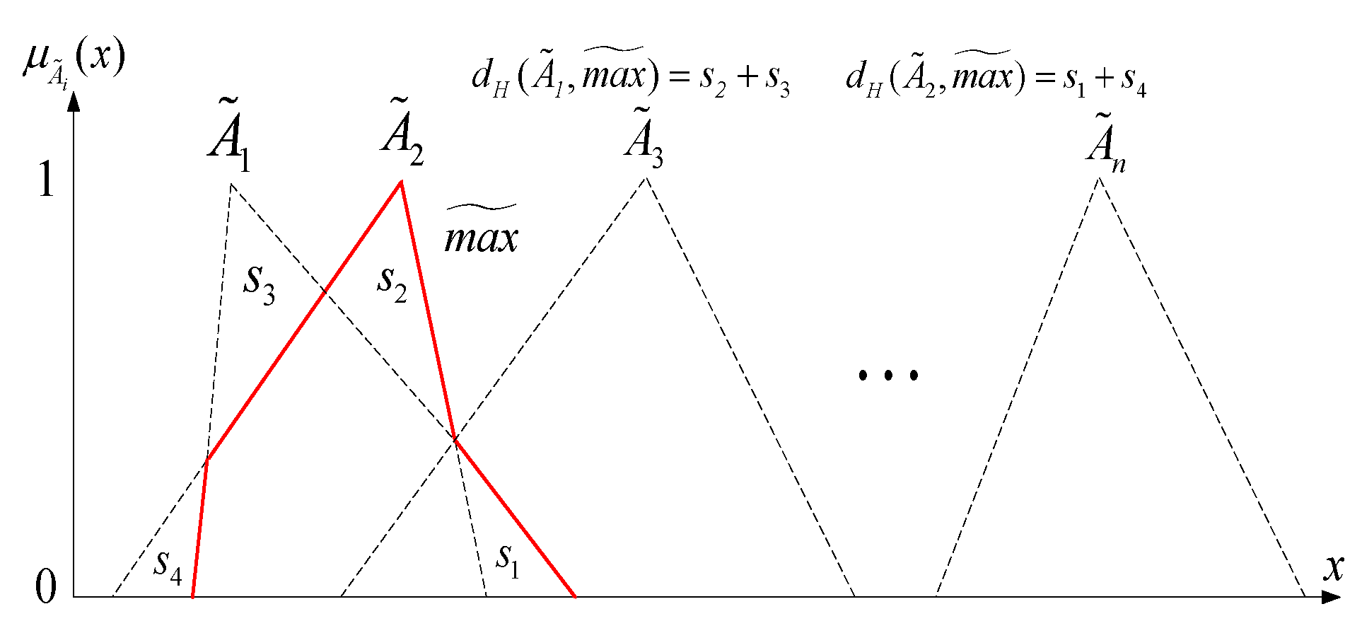
In this paper, a triangular fuzzy number $\tilde{A}$ can be defined as $\tilde{A}=(l,m,r)$, the membership function of which is defined as:

$$\begin{array}{c}\hfill {\mathsf{\mu }}_{\tilde{A}\left(x\right)}=\left\{\begin{array}{c}(x-l)/(m-l)l<x\le m\hfill \\ (r-x)/(r-m)m<x\le r\hfill \\ 0\text{otherwise}\hfill \end{array}\right.\end{array}$$

(34)

where l and r are the lower and upper limits of the fuzzy number $\tilde{A}$, and m is the modal value. The membership function of the triangular fuzzy number $({\tilde{A}}_1,{\tilde{A}}_2,\cdots ,{\tilde{A}}_n)$ can be illustrated as in Figure 2.

Where the red thick lines in Figure 3 represent the membership function of the maximum fuzzy subset $\widetilde{\text{max}}$ between $\widetilde{A_1}$ and $\widetilde{A_2}$. Define ${\tilde{A}}_{\text{max}}=\widetilde{\text{max}}({\tilde{A}}_1,{\tilde{A}}_2,\cdots ,{\tilde{A}}_n)$ as the maximum fuzzy subset among $({\tilde{A}}_1,{\tilde{A}}_2,\cdots ,{\tilde{A}}_n)$, the membership function of ${\tilde{A}}_{\text{max}}$ is defined as:

$${\mathsf{\mu }}_{{\tilde{A}}_{\text{max}}}\left(x\right)=\underset{\begin{array}{c}{x}_1\vee x_2\vee \cdots \vee x_n\hfill \\ (x_1,x_2,\cdots ,x_n)\in R^n\hfill \end{array}}{sup}min\left\{{\mathsf{\mu }}_{{\tilde{A}}_1}\left(x_1\right),{\mathsf{\mu }}_{{\tilde{A}}_2}\left(x_2\right),\cdots ,{\mathsf{\mu }}_{{\tilde{A}}_n}\left(x_n\right)\right\}$$

(35)

Hamming distance [24] $d_H({\tilde{A}}_i,{\tilde{A}}_j)$ is used here to measure the distance between two fuzzy numbers ${\tilde{A}}_i$ and ${\tilde{A}}_j$:

$$d_H({\tilde{A}}_i,{\tilde{A}}_j)={\int }_{x\in R}\left|{\mathsf{\mu }}_{{\tilde{A}}_i}\left(x\right)-{\mathsf{\mu }}_{{\tilde{A}}_j}\left(x\right)\right|dx$$

(36)

The hamming distance $d_H({\tilde{A}}_1,\widetilde{\text{max}})$ and $d_H({\tilde{A}}_2,\widetilde{\text{max}})$ are illustrated in Figure 3, where $s_1$,$s_2$,$s_3$, and $s_4$ are the geometric metric of hamming distance. $d_H\left({\tilde{A}}_1,\widetilde{\text{max}}\right)=s_2+s_3$, $d_H\left({\tilde{A}}_2,\widetilde{\text{max}}\right)=s_1+s_4$.

In this paper, the pseudo code of the proposed FODM algorithm is shown as follows:

Algorithm 2 FODM

1: Initialization: $f_{i,Jk}$=rep(i).Cost(k), i=(1,2,⋯,m), k=(1,2,3,4), $\tilde{\mathsf{\omega }}=({\tilde{\mathsf{\omega }}}_1,{\tilde{\mathsf{\omega }}}_2,{\tilde{\mathsf{\omega }}}_3)$, ${\tilde{\mathsf{\omega }}}_k=(a;\mathsf{\alpha },\mathsf{\beta })$, $f_{Jk}^{\min }=min(f_{1,Jk},f_{2,Jk},\cdots ,f_{m,Jk})$ 2: Build triangle fuzzy number matrix: ${\tilde{f}}_{i,Jk}=(f_{i,Jk},f_{i,Jk},f_{i,Jk})$ $$\tilde{P}=\left[\begin{array}{ccc}{\tilde{f}}_{1,J1}& {\tilde{f}}_{1,J2}& {\tilde{f}}_{1,J3}\\ {\tilde{f}}_{2,J1}& {\tilde{f}}_{2,J2}& {\tilde{f}}_{2,J3}\\ ⋮& ⋮& ⋮\\ {\tilde{f}}_{m,J1}& {\tilde{f}}_{m,J2}& {\tilde{f}}_{m,J3}\end{array}\right]$$ 3: Normalize the fuzzy matrix $\tilde{P}$: ${\overline{f}}_{i,Jk}=(c;\mathsf{\delta },\mathsf{\gamma })=(\frac{f_{Jk}^{\text{min}}}{f_{i,Jk}},\frac{f_{Jk}^{\text{min}}}{f_{i,Jk}},\frac{f_{Jk}^{\text{min}}}{f_{i,Jk}}\wedge 1)$ 4: Weighted $\tilde{P}$: ${\tilde{r}}_{ik}={\tilde{\mathsf{\omega }}}_k·{\overline{f}}_{i,Jk}=(ac;a\mathsf{\gamma }+a\mathsf{\alpha }-\mathsf{\alpha }\mathsf{\gamma },a\mathsf{\delta }+c\mathsf{\beta }-\mathsf{\beta }\mathsf{\delta })$ 5: Calculate the fuzzy ideal solution ${\tilde{M}}^{+}$: ${\tilde{M}}^{+}=({\tilde{M}}_1,{\tilde{M}}_2,{\tilde{M}}_3,{\tilde{M}}_4)$, ${\tilde{M}}_k=\widetilde{max}({\tilde{r}}_{1k},{\tilde{r}}_{2k},\cdots ,{\tilde{r}}_{mk})$ 6: Compute hamming distance: $D_i=\sqrt{{\displaystyle \sum _{k=1}^3}\left[d_H{({\tilde{r}}_{ik},{\tilde{M}}_k^{+})}^2\right]}$ 7: Sort Di from small to large, the smallest is the best compromise solution.

5. Case Study and Results

5.1. Case Study

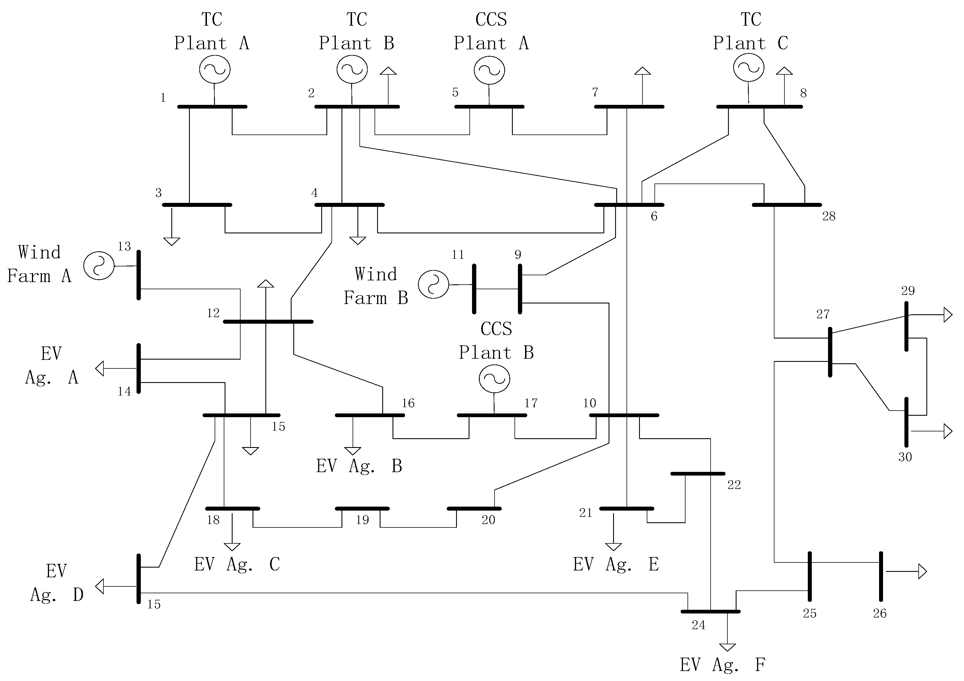
In this work, a 30 node grid system as shown in Figure 3 is adopted here to verify the effectiveness of the proposed optimal strategy, which contains two CCS thermal plants, three TC thermal plants, two wind farms, and six EV aggregators. Where the capacity of TC thermal plants is 150 MW, the capacity of CCS thermal plant is 150 MW, the capacity of a wind farm is 100 × 2 MW. There are 1000 EV in each EV aggregator, while the capacity of each EV’s battery is 200 kWh. The upper limit of charging power is 40 kW, while the upper limit of discharging power is also 40 kW. Assuming the SOC of the 1000 EV is in accord with Gaussian distribution, set $SO{C}_{i,\mathrm{d\hspace{0.17em}}\text{min}}^{\mathrm{D}}=SO{C}_{i,\mathrm{c\hspace{0.17em}}\text{max}}^{\mathrm{C}}=50\%$. Assuming EV’s charging price ${\mathsf{\gamma }}_{i,k}^{\mathrm{C}}=0.1\$/kWh$, EV’s discharging cost ${\mathsf{\gamma }}_{i,k}^{\mathrm{D}}=0.2\$/kWh,$ EV’s battery degradation cost $\zeta =0.13\$/kWh$ [2]. Simulation Parameters of the used thermal plants are listed as shown in

Table 1. Simulation parameters of the used thermal plants.

Plants	${\mathit{P}}_{\mathit{i},\mathit{k}}^{\mathbf{\text{max}}}$	${\mathit{P}}_{\mathit{i},\mathit{k}}^{\mathbf{\text{min}}}$	${\mathit{U}}_{\mathbf{G}}$	${\mathit{D}}_{\mathbf{G}}$	${\mathit{a}}_{\mathit{i}}$	${\mathit{b}}_{\mathit{i}}$	${\mathit{c}}_{\mathit{i}}$	${\mathsf{\alpha }}_{\mathit{i}}$	${\mathsf{\beta }}_{\mathit{i}}$	${\mathsf{\pi }}_{\mathit{i}}^{\mathbf{e}}$	${\mathsf{\pi }}_{\mathit{i}}^{\mathbf{s}}$	ω
TC Plant	150	20	–1.5	1.5	0.013	23.07	1675	0.63	5	10
CCS Plant	150	20	–1.5	1.5	0.017	32.31	2178	0.63	5	10	5	85

.

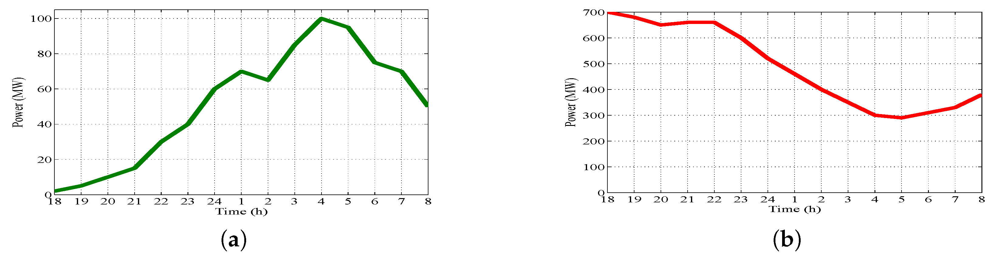
In this paper, the wind power model is predicted as Figure 4a shows, while the wind farm operating cost factor ${\epsilon }_i$ is 50 $/MW, and the reserve coefficient of wind turbines, $w\%$, is 20%.

In order to reduce the risk of incorporating uncertain wind forecasts into system scheduling, wind uncertainty should be taken into consideration before conducting further calculation. It is assumed that the wind forecast error is likely normally distributed [28]. The error of wind generation forecast is referred to as $\tilde{e}$. The forecasting error is estimated with a level of confidence $\mathsf{\alpha }\%$ [29], which means the probability of forecasting error being greater or equal to $\tilde{e}$ is less than $(100-\mathsf{\alpha })\%$. The wind generation capacity counted in the optimal schedule is calculated by:

$$P_{\text{wc},i}^k=\left\{\begin{array}{ll}{P}_{\text{wp},i}^k-\tilde{e}& \left(P_{\text{wp},i}^k\ge \tilde{e}\right)\\ 0& \left(P_{\text{wp},i}^k<\tilde{e}\right)\end{array}\right.$$

(37)

where $P_{\text{wp},i}^k$ is the predicted wind power generation of wind farm i.

Since we are concerned more with overestimation of the wind power (or that the power supply might not satisfy the demand), a one-side distribution curve is considered. By specifying the level of confidence, the value of $\tilde{e}$ can be estimated as follows:

$$P\left(\frac{e-{\mathsf{\mu }}_{\mathrm{e}}}{{\mathsf{\sigma }}_{\mathrm{e}}}\le z_{\mathsf{\alpha }}\right)=\left(100-\mathsf{\alpha }\right)\%$$

(38)

$$\tilde{e}={\mathsf{\mu }}_{\mathrm{e}}+z_{\mathsf{\alpha }}{\mathsf{\sigma }}_{\mathrm{e}}$$

(39)

where ${\mathsf{\mu }}_{\mathrm{e}}$ and ${\mathsf{\sigma }}_{\mathrm{e}}$ are the estimated mean value and standard deviation from sampling of the error of the historical forecast, respectively. The value of $z_{\mathsf{\alpha }}$ for 90%, 95%, and 99% confidence level can be chosen by

Table 2. Select of z_α value.

P[(e − μe) ≥ zασe] = α%	90%	95%	99%
zα	1.285	1.645	2.329

[29].

In the simulation setup of this paper, the confidence level is selected as 95%, the error mean ${\mathsf{\mu }}_{\mathrm{e}}$ is 5 MW, and the standard deviation ${\mathsf{\sigma }}_{\mathrm{e}}$ is 3 MW.

Assuming that the system load model is as Figure 4b shows while there are no EVs in the EV aggregator. Assuming that the reserve coefficient of system load L% is 10%.

MOPSO parameters are initialized as follows: both the maximum number of iterations and population size are set to 200, while repository size is set to 50, inertia weight ω is 0.5, the personal learning coefficient $c_1$ is 1, while the global learning coefficient $c_2$ is 1.

5.2. Results and Analysis

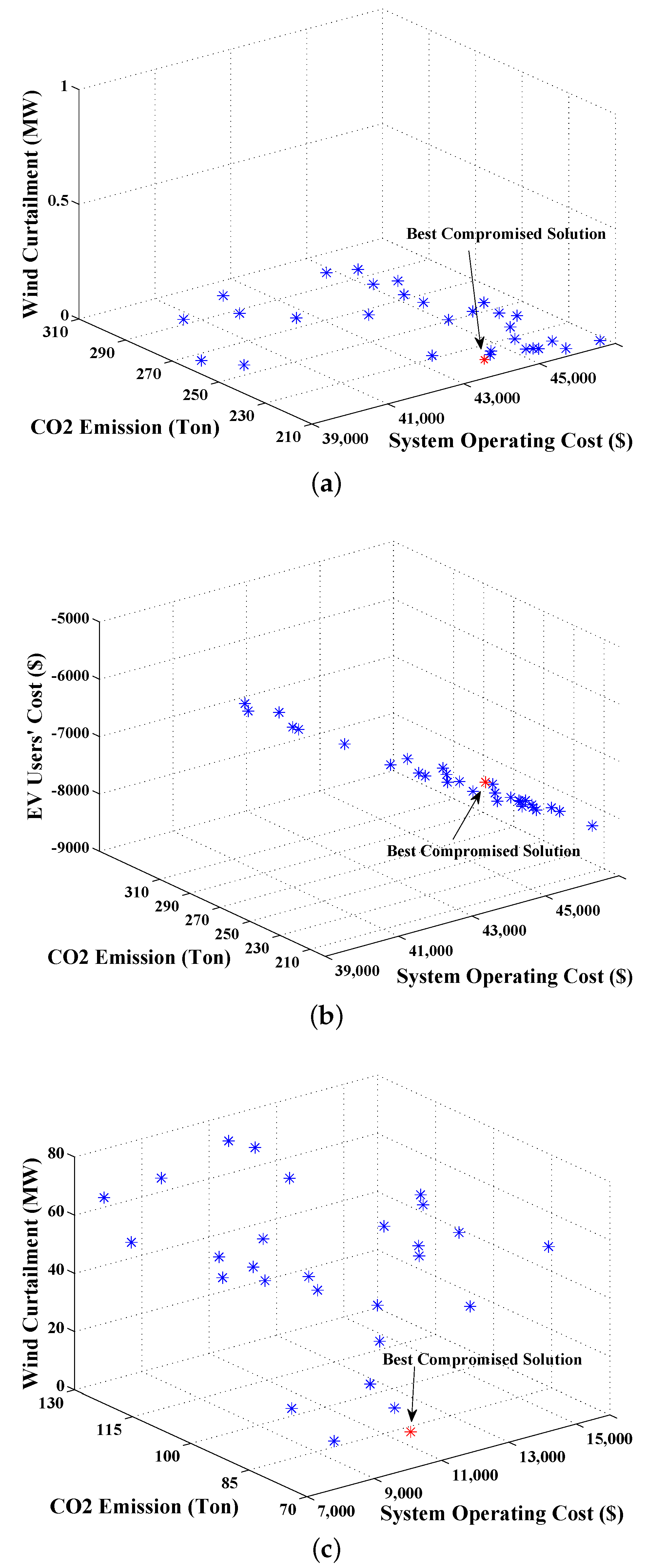
According to the above curve and installment, the data of system operating status at 18:00, 1:00, and 4:00 are extracted out respectively to calculate the result of the simulation case. The cost of TC plants and CCS plants is calculated by using Equations (12) and (14), respectively, the emission of TC plants and CCS is calculated by using Equations (13) and (15). Equation (16) is used to calculate the amount of captured amount of CO₂ of CCS plants. Equation (22) is used to calculate the wind farms’ cost, while EV’s charging and discharging cost is calculated by using Equations (2) and (3). Equations (24)–(27) are used to calculate the global cost, CO₂ emission, wind curtailment, and EV users’ cost, respectively. These equations are subject to the aforementioned constraints.

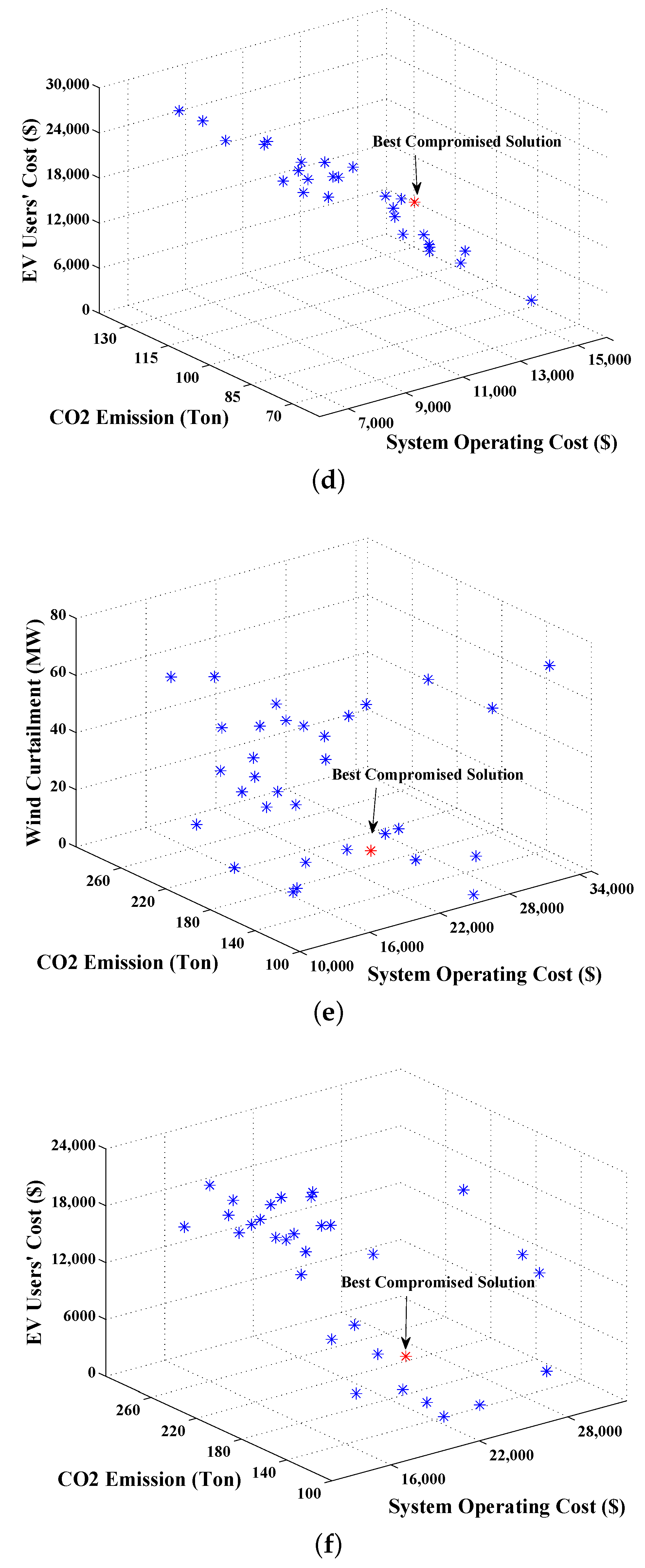
The Pareto front of the three scenes are shown as shown in Figure 5.

Setting up the fuzzy weight of the four objective functions by using triangle fuzzy members “Middle” ( ${\tilde{\mathsf{\omega }}}_1=(0.3,0.4,0.5)$ ), “High” ( ${\tilde{\mathsf{\omega }}}_2=(0.4,0.5,0.6)$), “High” ( ${\tilde{\mathsf{\omega }}}_3=(0.4,0.5,0.6)$) and “Middle” ( ${\tilde{\mathsf{\omega }}}_3=(0.3,0.4,0.5)$) (the way to calculate it is shown as pseudo code in Section 4.2) respectively, the individual of the highest fuzzy optimality which is also the best compromised solution is selected from the Pareto front as

Table 3. Best compromised solutions at different times.

Variables and Objectives	18:00	4:00	1:00
TC plants power (MW)	297.2	102.2	199.8
CCS Plants power (MW)	299.2	106.7	174.6
Wind farms power (MW)	0	176.9	105.7
EV aggregators discharging power (MW)	104.5	0	13.56
EV aggregators charging power (MW)	0	85.83	33.64
System operating cost ($)	44,230	11,194	20,707
CO2 Emission (ton)	221	80	148
Wind cultailment (MW)	0	3	14
EV user’s cost ($)	–7138	19,673	6787

shows.

By contrasting Figure 5 and Table 3, it can be seen that:

From the above case it can be seen that when the system load is relatively high, for example at 18:00 (due to the fact that wind energy is relatively low by that time), the thermal plants need to go all-out to satisfy the power needs of the load in the system. However, when the EV aggregator is controlled to discharge its power to the grid, it is capable of sharing part of the thermal plants’ work, hence the CO₂ emission can be relatively cut down. Also, EV users can receive economy benefit from sending their EVs to attend the V2G activity at the same time.

As a contrast, when the system load is relatively low, for example in the 1:00 scenario (due to the relatively high availability of wind energy at that time), while the thermal plants still need to maintain spinning, a large amount of wind energy will be abandoned for keeping the power balance of the grid. However, this power was saved because the EV aggregator is controlled to charge from the grid by the time. Hence, the wind curtailment of the system is reduced.

Table 4. Contrast of two strategies under different discharging prices at 18:00.

EV discharging cost ${\mathsf{\gamma }}_{i,k}^{\mathrm{D}}$ ($/kWh)	0.05	0.1	0.2
EV aggregators discharging power A (MW)	119.8	109.5	69.98
EV aggregators discharging power B (MW)	83.03	81.57	104.5
System operating cost A ($)	25,582	30,072	37,947
System operating cost B ($)	27,167	31,832	44,230
EV user’s cost A ($)	19,988	16,288	–4431
EV user’s cost B ($)	9641	3456	–7138
CO2 emission A (ton)	252	264	257
CO2 emission B (ton)	249	244	221

shows the result of a contrast simulation of two strategies under different discharging prices in the 18:00 scenario. One does not take the EV user’s cost into consideration (strategy A), while another is the proposed strategy in this paper (strategy B).

Table 5. Contrast of two strategies under different charging prices at 4:00.

EV charging cost ${\gamma }_{i,k}^{\mathrm{C}}$ ($/kWh)	0.1	0.2	0.5
EV aggregators charging power A (MW)	118.1	119.6	120
EV aggregators charging power B (MW)	85.83	80.76	67
System operating cost A ($)	8973	–3316	–39,287
System operating cost B ($)	11,194	2881	–14,480
EV user’s cost A ($)	27,163	39,435	75,600
EV user’s cost B ($)	19,673	26,606	42,179
Wind curtailment A (MW)	1.3	1	2
Wind curtailment B (MW)	3	6	21

shows the result of a contrast simulation of strategies A and the proposed strategy in this paper (strategy B) under different charging prices in the 4:00 scenario.

From Table 4 it can be seen that when the EV users’ cost is not considered, EVs discharge more energy when the discharging price ${\mathsf{\gamma }}_{i,k}^{\mathrm{D}}$ is lower, and discharge less energy when the discharging price is higher. This is because a higher discharging price means the grid company needs to pay more money to EV users, which will increase the grid operating cost. However, if the discharging price is too low, even below the charging price, EVs might discharge energy to charge itself while the battery degradation cost is not taken into consideration. This will definitely lead to an increase on EV user’s cost, which is unacceptable for EV users since the they wish to achieve economy benefits from attending V2G activity. The advantage of strategy B (proposed in this paper) is, because the user’s cost is taken into consideration while conducting system optimization, a compromised solution between system operating cost and EV users’ cost will be chosen by using FODM. The system will not reduce the EVs’ discharging power when the discharging price is relatively high (e.g., in the peak load period), and will limit EVs’ discharging power when the discharging price is too low. As a result, CO₂ emission is reduced and the willing of EV users to attend the V2G activity is enhanced.

From Table 5 it can be seen that EVs’ charging power is relatively high while EV users’ cost is not taken into consideration. This is because a higher charging price means more income from EV users to the grid company, the system operating cost will also drop if the charging price is increasing. However, it is unacceptable for EV users if the charging price is too high. By using strategy B, system will drop part of the wind power and limit EV’s charging power when the charging price is too high. Hence, the interest of EV users is protected. Otherwise, due to strategy B taking battery degradation cost into consideration inside its objective function, the charging power of strategy B will not be as high as that of strategy A.

6. Conclusions

This paper presents a dynamic environmental dispatch model which coordinates a cluster of charging and discharging controllable EV units with large-scale wind power farms and large thermal plants. A MOPSO algorithm for the optimization of system operating costs, CO₂ emissions, wind curtailment, and EV user’s cost is presented to obtain the Pareto front of the optimization problem and a FODM method is proposed then to extract out the best compromise solution from the Pareto optimal set. The simulation results further demonstrate that the best compromised solution calculated by the proposed strategy is able to schedule charging and discharging of EV aggregator to balance supply and demand for active power, according to grid status. System operating costs, CO₂ emissions, and wind curtailment can be relatively reduced and the objective of EV users’ cost is demonstrated to be able to ensure the interest of EV users attending V2G activity. The contribution of the proposed method can be described as follows: (1) establishing a mathematical model of wind farms, EV aggregators, and thermal plants while considering many operating constrains and security requirements; (2) using MOPSO as the solver to deal with the proposed MOP; (3) proposed a FODM-based algorithm to extract out the compromised best solution of the Pareto Front; (4) take EV users’ cost into consideration in the optimization model, thus a best compromised solution between system operating cost, EV users’ cost, CO₂ emission, and wind curtailment is obtained.