An Innovative Control Strategy to Improve the Fault Ride-Through Capability of DFIGs Based on Wind Energy Conversion Systems

Abstract

An innovative control strategy is proposed for enhancing the low voltage ride-through (LVRT) capability of a doubly fed induction generator based on wind energy conversion systems (DFIG-WECS). Within the proposed control method, the current control loops of the rotor side converter (RSC) are developed based on passivity theory. The control scheme for the grid side converter (GSC) is designed based on a two-term approach to keep the DC-link voltage close to a given value. The first term based on the maximal voltage of GSC is introduced in the GSC control loops as a reference reactive current. The second one reflecting the instantaneous unbalanced power flow between the RSC and GSC is also introduced in the GSC control loops as a disturbance considering the instantaneous power of the grid filter to compensate the instantaneous rotor power. The effectiveness of the proposed control strategy is verified via time domain simulation of a 2.0 MW-575 V DFIG-WECS using PSCAD/EMTP. Simulation results show that the control of the DFIG with the proposed approach can improve the LVRT capability better than with the conventional one.

1. Introduction

The wind industry set a new record for installations in 2014 after a slowdown during the past few years. Globally, 51,473 MW of new wind power installation were added. The global total generation capacity could reach 600 GW by the end of 2018 [1]. Currently, there are 103 countries using wind power on the commercial basis, among which China continues to be the main driver of wind market growth because its total capacity of 114,609 MW reached by the end of 2014. According to the World Wind Energy Association, top markets in the world include China, Germany, Spain and India, in which China passes the 100 GW of wind energy installed mark. With the increasing penetration level of wind energy in power systems, more and more responsibilities must be assumed for the operation of wind farms with respect to the electrical system [2]. In consequence, wind energy conversion systems (WECS) should be kept stable under the various operating conditions of the system when they are connected to the power grid.

The wind turbine technology using doubly fed induction generators based on wind energy conversion systems (DFIG-WECS) is widely used in the current wind energy industry compared with the other types because of its technical and economic advantages [3,4,5]. For example, it can absorb more wind energy than other types when the wind speed is below the rated value, and the cost of the power converters and harmonic filters is lower. Moreover, for wind generation based on doubly fed induction generator (DFIG) systems, power losses at the converters are lower than for the other systems based on the synchronous generators with full-rated converters. Therefore, the DFIG is an appropriate choice for the wind energy market.

Fundamentally, the DFIG consists of a wound rotor induction generator (WRIG) together with slip rings and a back-to-back voltage source converter (VSC), in which the WRIG rotor is connected to the grid through a back-to-back converter, while the stator is directly connected to one [6]. The power converter of the generator side, called the rotor side converter (RSC), is employed to control the reactive and active power or the torque of the generator. On the other hand, the power converter of the grid side is called grid side converter (GSC), and it is employed to maintain the DC link voltage and control reactive power compensation into the grid. The variable speed allows changing between ±30% around the synchronous speed, such that the VSC system needs to process a rate of approximately 30% to the rating of the wind turbine. The required VSC rating is smaller than the total rating of generator, but it depends on the selected speed variable range of generator. However, any increase in the speed variable range results in a corresponding increase of the size and cost of VSC [7].

The main drawback of DFIG-WECS systems is that they are very sensitive to grid disturbances, especially under voltage dip conditions. When an external grid fault occurs, a voltage dip is produced at the generator terminal, resulting in over-voltages and currents in the rotor and stator circuits and over-voltages in the DC-link because negative sequence components exist in the stator voltage. This can cause damages to the VSC, DC-link capacitor and other parts of the generator-turbine system and cause a temporary loss of the control of the active and reactive power of the DFIG’s rotor converter. Considering the continuous increase in wind power capacity, the grid connection codes of many countries were modified such that for a wind turbine to be FRT capability, it must not only remain connected to the grid during faults, but also control active and reactive power should be maintained [2]. This is motivated by the fact that disconnecting a large amount of wind power generation can cause the instability of the power system. Therefore, the control of DFIG-WECS represents a difficult task and a major challenge for equipment manufacturers as well as researchers.

Based on these facts, many papers have presented new control strategies to enhance the FRT performance of the DFIG-WECS. Extra protective hardware or proper control strategies are used [8,9]. A control strategy based on coordination between the conventional crowbar protection and the chopper circuit was introduced in [10]. The main idea is to disconnect the RSC, so the generator and the converters can be protected, but the controllability of the active and reactive power of the rotor converter is temporarily lost and the DFIG acts as conventional induction generator that consumes the reactive power from the network when the RSC is deactivated. Moreover, the cost of the device increases and the reliability decreases. In [11,12,13] the authors have suggested modifying the hardware and installing a series grid side converter (SGSC). However, these can increase the complexity of control systems and the cost of the device itself. The use of flexible alternating current transmission systems (FACTS) devices is proposed in [14,15,16] to improve the FRT capability. Obviously, these studies only focus on verifying the support of FACTS under dynamic responses of the wind turbines. The demagnetizing method is introduced in [17]; this method is used to suppress the electromagnetic transients in the rotor circuit and counteract the stator flux fluctuations during a grid fault with the main objective of decreasing the rotor current. However, the control of RSC is too complicated to be performed practically in industries. The authors of [18,19] have proposed a control strategy for RSC and GSC based on existing characteristics within the DFIG-WECS system to enhance the low voltage ride-through (LVRT) without using extra protective hardware. However, the exchanged power in the grid filter impedance during the grid faults is ignored. According to the authors in [20], the influences of the interface grid side filter are relatively large with respect to a high power DFIG.

This paper proposes a novel control strategy for both the RSC and GSC, which makes full use of existing properties within the DFIG-WECS to enhance the LVRT capability of DFIG-WECS without the need for additional protection devices. The proposed control strategy for RSC is designed by applying the passivity theory based on the non-linear properties of the generator to replace the PI controllers of the current control loop, so that the tracking properties of the mechanical and electrical reference values can be ensured. Therefore, the maximum wind energy is effectively captured; the speed and current of the generator are rapidly and exactly tracked to the desired values. For the GSC control strategy, the estimated rotor output power value is added in the GSC control loops as a feed-forward compensation signal of the active current with consideration of the instantaneous absorbed or delivered power of grid filter impedance during grid faults. The estimated reactive current value which is like a reference value is also introduced in the GSC control loops as a feed-forward signal based on the maximal rated voltage of the GSC.

The main objective of the proposed control strategy is to limit the DC-link voltage fluctuations, reduce the peak values of rotor and stator currents, and continuously supply active and reactive power to the grid during severe grid faults. The effectiveness of the proposed control strategy is verified via the time domain simulation of a 2.0 MW-575 V DFIG-WCES through the various scenarios based on the wind power grid connection codes. Simulation results are evaluated and compared with the conventional control strategy, in which the PI controllers and hardware protection devices are used.

The remainder of the paper is organized as follows: in Section 2, we explain the generator and wind turbine models. The behaviour of the DFIG-WECS under grid fault is presented in Section 3. In Section 4, we present the proposed control strategy. The case study and results are displayed in Section 5. Finally, the conclusions are given in Section 6 and the parameters of the controllers and studied system are listed in the Appendix A1 and Appendix A2.

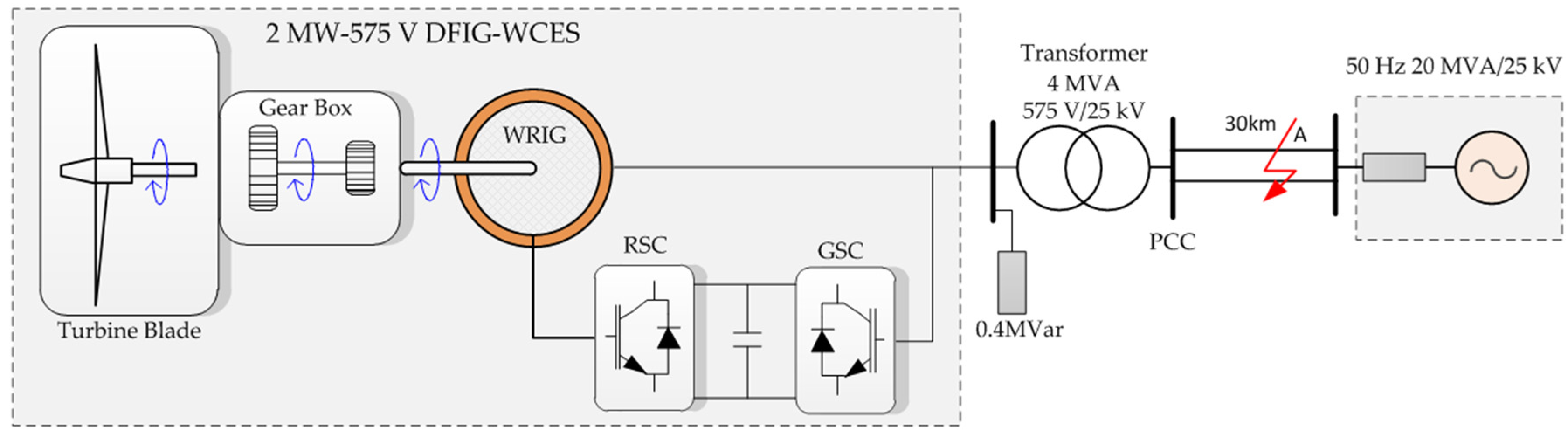
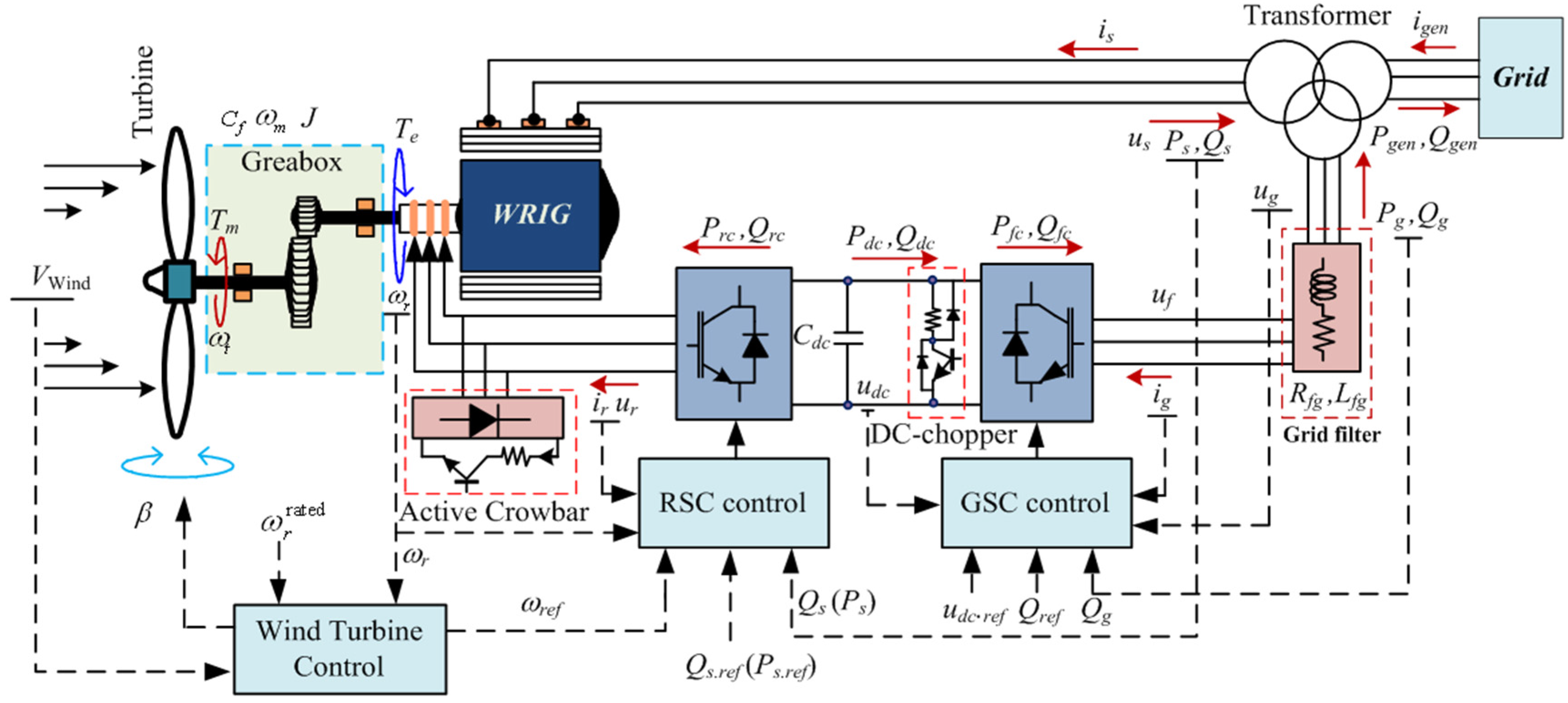
2. DFIG-WECS Model

2.1. WRIG

The configuration of a grid-connected DFIG-WECS system including a WRIG, WECS, back-to-back pulse width modulated (PWM) converter with a DC-link capacitor, control systems, protection systems, and pitch angle controller is shown in Figure 1. It is connected to the grid through a coupling transformer. The dynamic equations in the d-q reference frame of the WRIG can be described [21,22,23] by the voltages:

$$\{\begin{array}{l}{u}_{ds}=R_s{i}_{ds}-\mathsf{\omega }{\mathsf{\lambda }}_{qs}+\frac{d}{dt}{\mathsf{\lambda }}_{ds}\\ u_{qs}=R_s{i}_{qs}+\mathsf{\omega }{\mathsf{\lambda }}_{ds}+\frac{d}{dt}{\mathsf{\lambda }}_{qs}\\ u_{dr}=R_r{i}_{dr}-(\mathsf{\omega }-{\mathsf{\omega }}_r){\mathsf{\lambda }}_{qr}+\frac{d}{dt}{\mathsf{\lambda }}_{dr}\\ u_{qr}=R_r{i}_{qr}+(\mathsf{\omega }-{\mathsf{\omega }}_r){\mathsf{\lambda }}_{dr}+\frac{d}{dt}{\mathsf{\lambda }}_{qr}\end{array}$$

(1)

where subscripts s and r denote the stator and rotor quantities, respectively. Subscripts d and q denote the d- and q-axis components, respectively; ω is the speed of the d-q reference frame; R is the resistance, u, i and λ are the voltage, current, and flux, respectively; ω_r = pω_m is the rotor angular frequency, where ω_m is rotor mechanical speed and p is number of pole pairs.

The flux linkages:

$$\{\begin{array}{l}{\mathsf{\lambda }}_{ds}=(L_{ls}+L_m)i_{ds}+L_m{i}_{dr}=L_s{i}_{ds}+L_m{i}_{dr}\\ {\mathsf{\lambda }}_{qs}=(L_{ls}+L_m)i_{qs}+L_m{i}_{qr}=L_s{i}_{qs}+L_m{i}_{qr}\\ {\mathsf{\lambda }}_{dr}=(L_{lr}+L_m)i_{dr}+L_m{i}_{ds}=L_r{i}_{dr}+L_m{i}_{ds}\\ {\mathsf{\lambda }}_{qr}=(L_{lr}+L_m)i_{qr}+L_m{i}_{qs}=L_r{i}_{qr}+L_m{i}_{qs}\end{array}$$

(2)

where L, L_l and L_m are self-inductance, leakage inductance, and mutual inductance, respectively.

Finally, electromagnetic torque:

$$T_e=\frac{3}{2}p(i_{qs}{\mathsf{\lambda }}_{ds}-i_{ds}{\mathsf{\lambda }}_{qs})$$

(3)

Figure 1. Schematic diagram of the DFIG-WECS.

Figure 1. Schematic diagram of the DFIG-WECS.

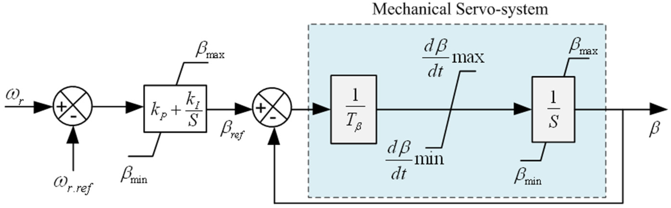
2.2. Wind Turbine

A wind turbine is used to convert the wind’s kinetic energy into mechanical energy that is then transformed into electric energy by a generator. The generator-turbine system is shown in Figure 1. The two-mass drive train model, including the gearbox, shafts, and other mechanical components of the wind turbine (WT), is often used to study the dynamic stability of DFIG-WECS. The shaft of generator rotor is connected to the shaft of turbine flexibly via gearbox and coupling [24]. The electromechanical dynamics of the generator-turbine system are presented by the following equations [25]:

$$2J\frac{d{\mathsf{\omega }}_m}{dt}=T_m-T_e-C_f{\mathsf{\omega }}_m$$

(4)

$$T_m=\frac{P_m}{{\mathsf{\omega }}_t}$$

(5)

where P_m and T_m are the mechanical power and torque of the wind turbine, respectively, C_f is the frictional coefficient, J is the inertia of the generator-turbine system, and ω_t is the rotational speed of the turbine.

The mechanical power can be obtained by the following equations [26,27]:

$$P_m=\frac{1}{2}\mathsf{\rho }\mathsf{\pi }{\Re }^2{V}_w^3{C}_p(\mathsf{\beta },\mathsf{\lambda })$$

(6)

$$C_p(\mathsf{\beta },\mathsf{\lambda })={\displaystyle \sum _{i=0}^4{\displaystyle \sum _{j=0}^4{\mathsf{\alpha }}_{ij}{\mathsf{\beta }}^i{\mathsf{\lambda }}^j}}$$

(7)

$$\mathsf{\lambda }=\frac{{\mathsf{\omega }}_t\Re }{V_w}$$

(8)

where C_p(·) is the power coefficient, ℜ is the blade radius of the turbine, ρ is the air density, β is the pitch angle, V_w is the wind speed, λ is the dip speed ratio, and α_i,j are factors that can be found in [27].

In order to optimize the extracted power from incoming wind and limit over-power production at high wind speeds, the generator-turbine system is controlled by using the maximum power point tracking (MPPT) model with the pitch angle control scheme that is shown in Figure 2 [19]. When the wind speed is a range between the cut-in wind speed and low limit wind speed, the generator rotor reference speed ω_r,ref is set as minimum value ${\mathsf{\omega }}_r^{\min }$ to insure the generator slip that is smaller than 30%. When the wind speed is greater than the low limit wind speed and smaller than the rated wind speed, the generator is operated in the variable speed model. The maximum power is obtained by tracking ω_r,ref in the following equation:

$${\mathsf{\omega }}_{r.ref}=\sqrt[3]{\frac{P_m}{K_{opt}}}=\sqrt{\frac{T_m}{K_{opt}}}$$

(9)

where $K_{opt}=(1/2)({\Re }^2/{\mathsf{\lambda }}_{opt}^3)\mathsf{\rho }\mathsf{\pi }{C}_p^{\max }(\mathsf{\beta },\mathsf{\lambda })$ is the optimal constant of turbine; the pitch angle β is kept constant at β_opt that is usually equal to zero, while λ is adjusted to λ_opt according to different wind speeds by adapting the ω_r,ref. When the wind speed increases larger than the rated speed, the ω_r,ref is set as the rated value of the generator speed ${\mathsf{\omega }}_r^{\text{rated}}$. The over-power production is limited by adjusting the pitch angle; consequently, the over-speed of generator is also limited. This paper focuses on the minimum and maximum values of generator speed that are 0.7 p.u. and 1.1 p.u., respectively, taking into account the reliable operation range of generator, based on the inner control loops of RSC.

Figure 2. Schematic diagram of the pitch angle controller.

Figure 2. Schematic diagram of the pitch angle controller.

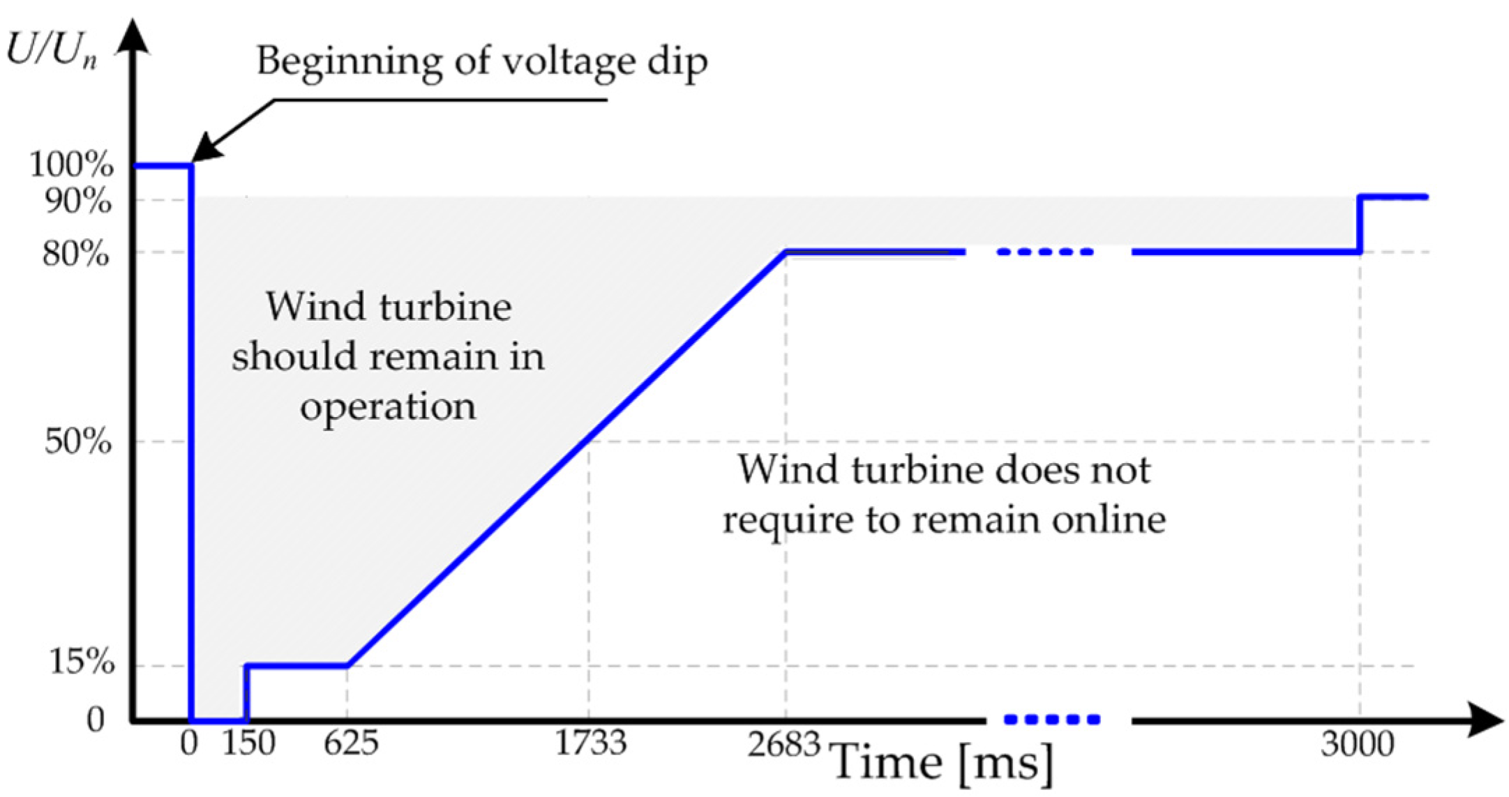
3. Behavior of the DFIG-WECS under Grid Fault Conditions

A grid fault appears at the point of common coupling (PCC) in the network, the voltage at PCC drops, resulting in the significant over-currents and voltages in the stator and rotor circuits because DC- and AC-components appear. In addition, the bi-directional power flow between the generator and grid via the rotor by a set of power converter becomes unbalanced. As a result, the transient voltage fluctuation in the DC-link can be increase significantly.

To demonstrate the protection schemes and their interaction with the rotor circuit, the rotor equivalent circuit is representative in the general Park’s model of induction generator. The stator flux evolution of generator is imposed by the stator voltage equation as [28]:

$${\overrightarrow{u}}_s=R_s{\overrightarrow{i}}_s+\frac{d{\overrightarrow{\mathsf{\lambda }}}_s}{dt}$$

(10)

$${\overrightarrow{\mathsf{\lambda }}}_s={\displaystyle \int \left({\overrightarrow{u}}_s-R_s{\overrightarrow{i}}_s\right)dt}$$

(11)

where ${\overrightarrow{u}}_s$, ${\overrightarrow{i}}_s$, and ${\overrightarrow{\mathsf{\lambda }}}_s$ are the stator voltage, current, and flux space vectors, respectively.

The equation of the rotor voltage is obtained as [29]:

$${\overrightarrow{u}}_r=\underset{{\overrightarrow{u}}_{ro}}{\underbrace{\frac{L_m}{L_s}(\frac{d{\overrightarrow{\mathsf{\lambda }}}_s}{dt}-j{\mathsf{\omega }}_r{\overrightarrow{\mathsf{\lambda }}}_s)}}+(R_r{\overrightarrow{i}}_r+L_r\mathsf{\sigma }(\frac{d{\overrightarrow{i}}_r}{dt}-j{\mathsf{\omega }}_r{\overrightarrow{i}}_r))$$

(12)

where ${\overrightarrow{i}}_r$ is the rotor current space vector and σ is the leakage coefficient, can be described as $\mathsf{\sigma }=1-L_m^2/L_s{L}_r$.

It can be seen that the first component of above equation is the electromotive force (EMF) caused by the stator flu ${\overrightarrow{\mathsf{\lambda }}}_s$, called the rotor open-circuit voltage ${\overrightarrow{u}}_{ro}$, which consists of a term $(L_m/L_s)(d{\overrightarrow{\mathsf{\lambda }}}_s/dt)$ that is created by the variation of the stator flux, and a term $j{\mathsf{\omega }}_r(L_m/L_s){\overrightarrow{\mathsf{\lambda }}}_s$ that is created by the rotating stator flux, can increase, if the stator flux contains DC-components. The second one is $R_r{\overrightarrow{i}}_r+L_r\mathsf{\sigma }(d{\overrightarrow{i}}_r/dt-j{\mathsf{\omega }}_r{\overrightarrow{i}}_r)$, represents the voltage dips in both the rotor resistance R_r and the transient inductance L_rσ, caused by the rotor current $\overrightarrow{i}$.

In normal operation, the stator voltage is a rotating vector and rotates at synchronous speed ${\mathsf{\omega }}_s$, can be expressed as:

$${\overrightarrow{u}}_s=U_s{e}^{j{\mathsf{\omega }}_{s}t}$$

(13)

where U_s is amplitude of the stator voltage.

Substituting Equation (13) into Equation (10) and neglecting the stator resistance R_s, we have:

$${\overrightarrow{\mathsf{\lambda }}}_s=\frac{U_s}{j{\mathsf{\omega }}_s}{e}^{j{\mathsf{\omega }}_{s}t}$$

(14)

Applying Equation (14) to Equation (12), the rotor open-circuit voltage is:

$${\overrightarrow{u}}_{ro}=\frac{L_m}{L_s}{U}_s(\frac{{\mathsf{\omega }}_s-{\mathsf{\omega }}_r}{{\mathsf{\omega }}_s})$$

(15)

where $s=\left({\mathsf{\omega }}_s-{\mathsf{\omega }}_r\right)/{\mathsf{\omega }}_s$ is the slip ratio.

Considering at time t = t₀, a symmetrical voltage dip appears in the power network suddenly, the stator voltage is reduced from normal amplitude U₁ to the faulty amplitude U₂. The stator voltages can be expressed as follows:

$${\overrightarrow{u}}_s=\{\begin{array}{l}{\overrightarrow{u}}_{s1}=U_1{e}^{j{\mathsf{\omega }}_{s}t}\mathrm{for}t<t_0\\ {\overrightarrow{u}}_{s2}=U_2{e}^{j{\mathsf{\omega }}_{s}t}\mathrm{for}t\ge t_0\end{array}$$

(16)

The stator fluxes before and after the voltage dip are:

$${\overrightarrow{\mathsf{\lambda }}}_s=\{\begin{array}{l}{\overrightarrow{\mathsf{\lambda }}}_{s1}=\frac{U_1}{j{\mathsf{\omega }}_s}{e}^{j{\mathsf{\omega }}_{s}t}\mathrm{for}t<t_0\\ {\overrightarrow{\mathsf{\lambda }}}_{s2}=\frac{U_2}{j{\mathsf{\omega }}_s}{e}^{j{\mathsf{\omega }}_{s}t}\mathrm{for}t\ge t_0\end{array}$$

(17)

Assuming open-circuit rotor $({\overrightarrow{i}}_r=0)$ and merging Equations (11) and (17), and the term ${\overrightarrow{\mathsf{\lambda }}}_s=L_s{\overrightarrow{i}}_s+L_s{\overrightarrow{i}}_r$, the stator flux of the machine during the whole grid fault period is expressed as:

$${\overrightarrow{\mathsf{\lambda }}}_s=\underset{{\overrightarrow{\mathsf{\lambda }}}_{s2}}{\underbrace{\frac{U_2}{j{\mathsf{\omega }}_s}{e}^{j{\mathsf{\omega }}_{s}t}}}+\underset{{\overrightarrow{\mathsf{\lambda }}}_{s0}}{\underbrace{\frac{U_1-U_2}{j{\mathsf{\omega }}_s}}}{e}^{-\frac{L_s}{R_s}t}$$

(18)

Equation (18) can be divided into two terms. The first one is the forced flux, which appears just after the voltage dip. The second one is the natural flux, which consists of a turning term ${\overrightarrow{\mathsf{\lambda }}}_{s0}$ that is determined based on the difference between the stator flux before and after the voltage dip occurs (from ${\overrightarrow{\mathsf{\lambda }}}_{s1}$ to ${\overrightarrow{\mathsf{\lambda }}}_{s2}$) and other term is the stator transient time constant of τ_s = L_s/R_s due to natural mode.

By merging Equation (12) with Equation (18), the dynamic behavior expression of the EMF is described in the rotor reference frame as follows:

$${\overrightarrow{u}}_r=\frac{L_m}{L_s}(s{U}_2{e}^{j\left({\mathsf{\omega }}_s-{\mathsf{\omega }}_r\right)t}-(1-s)(U_1-U_2)e^{-j{\mathsf{\omega }}_{r}t}{e}^{-\frac{L_s}{R_s}t})$$

(19)

Obviously, the first term of Equation (19) corresponds to the remaining stator voltage and slip ratio; its value is small because of proportionality to the slip ratio. The last one is proportional to term (1 − s); it depends on the depth of voltage dip and decays exponential function with the stator transient time constant of τ_s = L_s/R_s.

The maximum amplitude of the rotor voltage during grid fault can be obtained as:

$$U_{r\max }\approx \frac{L_m}{L_s}(\left|s\right|U_2-(1-s)(U_1-U_2))$$

(20)

If the depth of the voltage dip is small, the voltage caused by the stator flux does not exceed the maximal voltage of RSC; the control of RSC remains. For a larger voltage dip, then the voltage caused by the stator flux exceeds the maximal voltage of RSC, leading into the control of RSC being temporarily lost and the RSC is saturated. In this situation, the fluctuations of the rotor current and the stator flux are high, resulting in the increase of electromagnetic torque fluctuation. On the other hand, as shown from Equation (4), the mechanical torque changes slower than rotor speed and the rotor electrical speed oscillates during the grid voltage dip, leading to a significant fluctuation increase in the rotor voltage.

4. Proposed Control Strategy for the LVRT Capability of DFIG

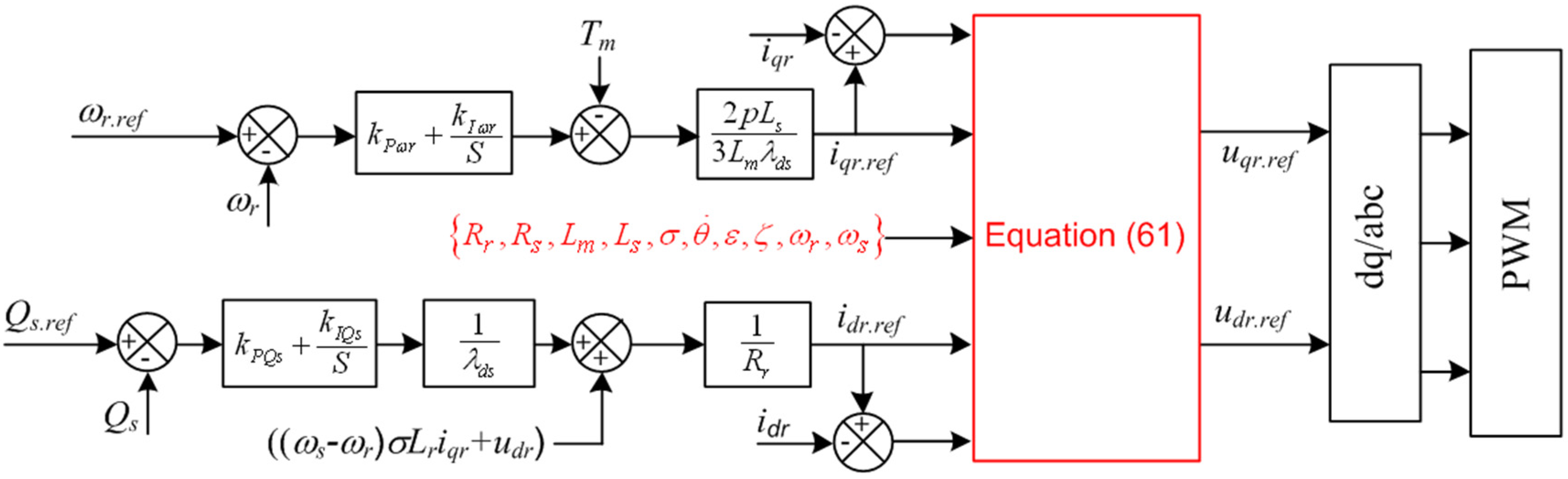
4.1. Control of RSC

The conventional control strategy of the RSC is illustrated in Figure 3. The decoupling of reactive power and electromagnetic torque control is performed using the vector control scheme based on the synchronous rotating d-q reference frame with the d-axis oriented along the stator-flux vector position [30]. The PI regulators with cascade control loops are used in the RSC control scheme, in which the outer control loops are for the reactive power and rotor speed regulation, and the inner control loops are for rotor side current regulation.

As analysed in Section 3, the difficulty of the LVRT control of the RSC is the prevention of the transient over-current on the rotor side of the DFIG that is induced by the voltage fluctuation in the DC-link and the transient electromotive force (EMF) of the rotor and stator fluxes. This subsection only focuses on the analyses of a novel control strategy for RSC that has been developed based on the non-linear model of the electric generator to replace the inner control loops. Thereby, the LVRT capability of the DFIG-WECS system can be improved. The control scheme diagram is illustrated in Figure 4.

Figure 3. The conventional control scheme of RSC.

Figure 3. The conventional control scheme of RSC.

Figure 4. The proposed control scheme of RSC.

Figure 4. The proposed control scheme of RSC.

4.1.1. Euler-Lagrange Equation and Passivity Property

Euler-Lagrange Equation for Electric Machine

The electric machine can be described as [31]:

$${\sum }_e:(u_{r.ref},{\mathsf{\omega }}_m)\mapsto (i_r,T_e)$$

(21)

$${\sum }_m:(T_m-T_e)\mapsto {\mathsf{\omega }}_m$$

(22)

where ${\sum }_e$, ${\sum }_m$ represent electrical and mechanical subsystems, respectively. $i_r=i_{dr}+j{i}_{qr}$ and $u_{r.ref}=u_{dr.ref}+u_{qr.ref}$ are the rotor current and voltage vectors, respectively.

The relationship between input and output of electrical system model is illustrated as shown in Figure 5b.

Figure 5. Nested-loop controller structure: (a) outer and inner control loops; (b) passive subsystem decomposition of generalized electric machine.

Figure 5. Nested-loop controller structure: (a) outer and inner control loops; (b) passive subsystem decomposition of generalized electric machine.

The Lagrange of the electric machine can be described as [32]:

$${\pounds }_e(i_r,\mathsf{\theta })=\frac{1}{2}{i}_r^{T}L(\mathsf{\theta })i_r$$

(23)

$${\pounds }_m(\dot{\mathsf{\theta }})=\frac{1}{2}J{\dot{\mathsf{\theta }}}^2$$

(24)

where ${\pounds }_e(i_r,\mathsf{\theta })$ and ${\pounds }_m(\dot{\mathsf{\theta }})$ are the Lagrange function of the electrical and mechanical subsystems, respectively. $\mathsf{\theta }={\displaystyle \int {\mathsf{\omega }}_m}dt$ is the rotor mechanical position. L(θ) is the electromagnetic inertia matrix.

Remark 1: 

Applying the Euler-Lagrange for Equation (23), the electrical subsystem is obtained as [31,33]:

$$\frac{d}{dt}(\frac{\partial {\pounds }_e(i_r,\mathsf{\theta })}{\partial i_r})=L(\mathsf{\theta })\frac{d{i}_r}{dt}+\dot{\mathsf{\theta }}\frac{\partial L(\mathsf{\theta })}{\partial (\mathsf{\theta })}{i}_r=L(\mathsf{\theta })\frac{d{i}_r}{dt}+\dot{\mathsf{\theta }}\frac{\partial L(\mathsf{\theta })}{\partial (\mathsf{\theta })}{i}_r$$

(25)

The electrical subsystem Equation (25) is driven by the input signal $M_e{u}_r$, we have:

$$L(\mathsf{\theta })\frac{d{i}_r}{dt}+\dot{\mathsf{\theta }}\frac{\partial L(\mathsf{\theta })}{\partial (\mathsf{\theta })}{i}_r+R{i}_r=M_e{u}_r$$

(26)

which is equivalent to:

$$\frac{d{\mathsf{\lambda }}_r}{dt}+R{i}_r=M_e{u}_r$$

(27)

where $M_e=\left[\begin{array}{l}{I}_2\\ 0\end{array}\right]$ is a constant matrix, $u_r$ is the control voltage vector, and $R=\left[\begin{array}{cc}{R}_s{I}_2& 0\\ 0& R_r{I}_2\end{array}\right]$ is the resistance matrix, with $I_2=\left[\begin{array}{cc}1& 0\\ 0& 1\end{array}\right]$ is unit matrix. In addition, $\frac{dL(\mathsf{\theta })}{dt}$ is expressed as:

$$\begin{array}{cc}\hfill \frac{dL(\mathsf{\theta })}{dt}=\dot{\mathsf{\theta }}\frac{\partial L(\mathsf{\theta })}{\partial (\mathsf{\theta })}& =\left[\begin{array}{cc}0& L_m{J}_2{e}^{J_2\mathsf{\theta }}\dot{\mathsf{\theta }}\\ -L_m{J}_2{e}^{{-J}_2\mathsf{\theta }}\dot{\mathsf{\theta }}& 0\end{array}\right]\hfill \\ & =\left[\begin{array}{cc}0& 0\\ -L_m{J}_2{e}^{-J_2\mathsf{\theta }}\dot{\mathsf{\theta }}& 0\end{array}\right]+\left[\begin{array}{cc}0& L_m{J}_2{e}^{J_2\mathsf{\theta }}\dot{\mathsf{\theta }}\\ 0& 0\end{array}\right]=C^T(\mathsf{\theta },\dot{\mathsf{\theta }})+C(\mathsf{\theta },\dot{\mathsf{\theta }})\hfill \end{array}$$

(28)

where $J_2=\left[\begin{array}{rr}0& -1\\ 1& 0\end{array}\right]$ is an anti-symmetric matrix.

Remark 2: 

Applying the Euler-Lagrange for Equation (24), the mechanical subsystem is obtained as [31,33]:

$$\frac{d}{dt}(\frac{\partial {\pounds }_m(\dot{\mathsf{\theta }})}{\partial \dot{\mathsf{\theta }}})=J\ddot{\mathsf{\theta }}$$

(29)

The mechanical subsystem Equation (29) is driven by the input signal (T_m − T_e), we have:

$$J\ddot{\mathsf{\theta }}=T_m-T_e$$

(30)

Hence, the electromagnetic torque of electric machine can be expressed as follows:

$$T_e=\frac{1}{2}{i}_r^T\frac{dL(\mathsf{\theta })}{dt}{i}_r$$

(31)

Passivity Property of DFIG

Proof 1: 

The DFIG’s property is a passivity system that is the basis to design the inner loops of RSC for DFIG.

The DFIG’s energy function can be expressed as follows:

$$E_{DFIG}=E_e+E_m=\frac{1}{2}{i}_r^{T}L(\mathsf{\theta })i_r+\frac{1}{2}J{\dot{\mathsf{\theta }}}^2$$

(32)

where E_e and E_m are the energy function of electrical and mechanical subsystems.

The energy of generator under variable speed is:

$$\frac{d{E}_{DFIG}}{dt}=i_r^T{u}_r-\dot{\mathsf{\theta }}{T}_m-i_r^{T}R{i}_r$$

(33)

By integrating both sides of Equation (33), the energy balance equation of the DFIG can be obtained as:

$$\underset{\mathrm{Stored}\mathrm{energy}}{\underbrace{E_{DFIG}(t)-E_{DFIG}(0)}}=\underset{\mathrm{Energy\; supplied}\mathrm{to}\mathrm{the}\mathrm{system}}{\underbrace{{\displaystyle \underset{0}{\overset{t}{\int }}(i_r^T{u}_r-\dot{\mathsf{\theta }}{T}_m)}}}-\underset{\text{Dissipated}}{\underbrace{{\displaystyle \underset{0}{\overset{t}{\int }}{i}_r^{T}R{i}_r}}}$$

(34)

We can show in Equation (34) that the energy of generator is smaller than the supplied energy from the system, this means that the mapping “$\left[u_r^T,-T_m\right]\mapsto \left[i_r^T,\mathsf{\theta }\right]$” is the passive relationship with respect to the stored energy total of DFIG. Hence, the DFIG’s property is perfectly passivity. This completes the proof.

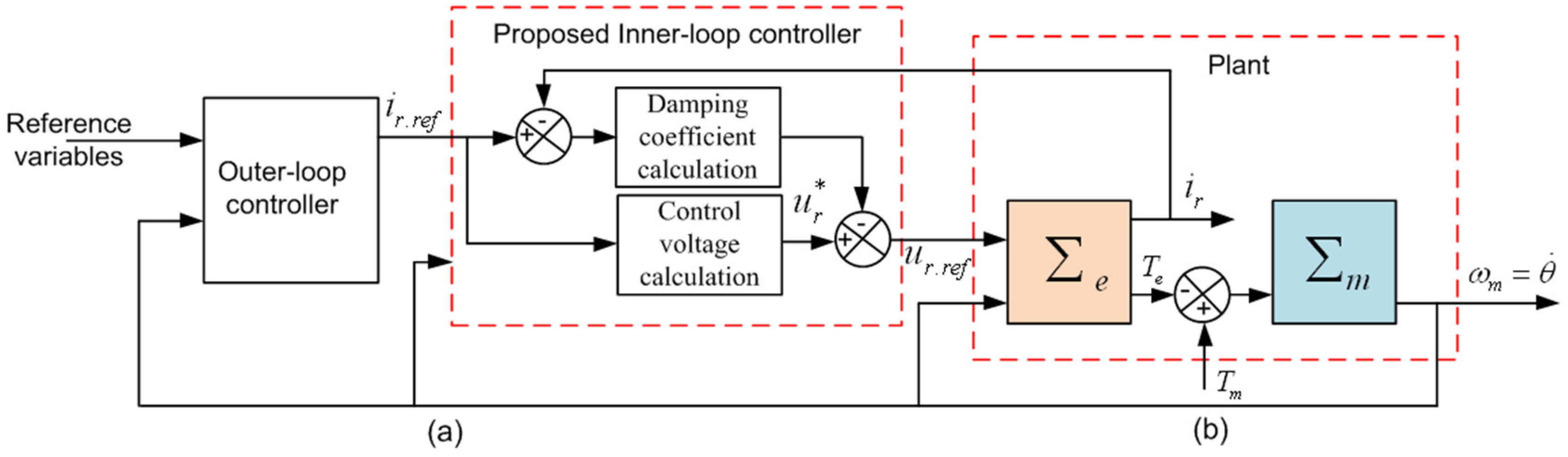
4.1.2. Design of Inner Control Loop

In order to limit the over-current in the rotor and stator circuits, maintain the DC-link voltage close to a given value, the damping coefficient should be injected into the control loops of RSC. Considering the reference value of rotor voltage (control signal) as follows:

$$u_{r.ref}=u_r-f(\dot{\mathsf{\theta }})i_r$$

(35)

where $f(\dot{\mathsf{\theta }})$ is the damping coefficient that will be determined in this subsection.

Substituting Equations (35) and (28) into Equation (26), we have:

$$L(\mathsf{\theta })\frac{d{i}_r}{dt}+C(\mathsf{\theta },\dot{\mathsf{\theta }})i_r+R_{f(\dot{\mathsf{\theta }})}{i}_r=M_e{u}_r$$

(36)

where $R_{f(\dot{\mathsf{\theta }})}$ can be defined as:

$$R_{f(\dot{\mathsf{\theta }})}=\left[C^T(\mathsf{\theta },\dot{\mathsf{\theta }})+R+\left[\begin{array}{l}f(\dot{\mathsf{\theta }})I_{2}0\\ 00\end{array}\right]\right]$$

(37)

based on Equation (28), the relationship between $L(\mathsf{\theta })$ and $C(\mathsf{\theta },\dot{\mathsf{\theta }})$ can be expressed as follows:

$$\frac{dL(\mathsf{\theta })}{dt}=C^T(\mathsf{\theta },\dot{\mathsf{\theta }})+C(\mathsf{\theta },\dot{\mathsf{\theta }})$$

(38)

Hence, Equation (36) can be expressed under the other form as follows:

$$x^T(\frac{dL(\mathsf{\theta })}{dt}-2C(\mathsf{\theta },\dot{\mathsf{\theta }}))x=0$$

(39)

The Equation (39) is an important property that is skew-symmetric, which is basis to design the inner control loop of RSC.

Proof 2: 

Injecting the damping coefficient into the control loops of RSC as shown in Equation (35) is to insure that output of system is perfectly passive with respect to the rotor voltage input, that is to say the stability of the created kinetic energy by electrical subsystem is perfectly independent from the kinetic energy created by the mechanical subsystem. Hence, we consider the storage energy function as follows:

$$\frac{d{E}_e}{dt}=i_r^{T}L(\mathsf{\theta })\frac{d{i}_r}{dt}+\frac{1}{2}{i}_r^T\frac{dL(\mathsf{\theta })}{dt}{i}_r$$

(40)

Based on Equation (39), we have:

$$i_r^T(\frac{dL(\mathsf{\theta })}{dt}-2C(\mathsf{\theta },\dot{\mathsf{\theta }}))i_r=0$$

(41)

Substituting Equation (41) into Equation (40), we have:

$$\frac{d{E}_e}{dt}=i_r^{T}L(\mathsf{\theta })\frac{d{i}_r}{dt}+i_r^{T}C(\mathsf{\theta },\dot{\mathsf{\theta }})i_r$$

(42)

Multiplying both sides of Equation (36) by $i_r^T$ and combining Equation (42), we have:

$$\frac{d{E}_e}{dt}=i_r^T{u}_r-i_r^T{R}_{f(\dot{\mathsf{\theta }})}{i}_r$$

(43)

By integrating of Equation (43), we have:

$$E_e(T)-E_e(0)={\displaystyle \underset{0}{\overset{T}{\int }}{i}_r^T{u}_r}dt-{\displaystyle \underset{0}{\overset{T}{\int }}{i}_r^T{R}_{f(\dot{\mathsf{\theta }})}{i}_r}dt$$

(44)

It can be observed from Equation (44), that the electrical subsystem is perfectly passive with the input control signal $u_r$. This completes the proof.

Proof 3: 

The electrical passivity system must track the desired electromagnetic torque, that is to say, the desired rotor current is calculated based on the rotor voltage input that it satisfies the conditions of $T_e^{*}=T_e$ and $i_{r.ref}=i_r$.

Lemma 1: 

There exists the rotor voltage input and the rotor reference current that they satisfy the rotor voltage function as follows:

$$\{\begin{array}{l}{M}_e{u}_r=L(\mathsf{\theta })\frac{d}{dt}{i}_{r.ref}+C(\mathsf{\theta },\dot{\mathsf{\theta }})i_{r.ref}+(R_{f(\dot{\mathsf{\theta }})}(\mathsf{\theta },\dot{\mathsf{\theta }}))i_{r.ref}\\ \underset{t\to \infty }{\lim }{\tilde{i}}_r=0\end{array}$$

(45)

where ${\tilde{i}}_r=(i_r-i_{r.ref})$ is the rotor current error and the superscript “*” denotes the desired value.

Lemma 2: 

Calculate $i_{r.ref}$, it must satisfy conditions $T_e^{*}=T_e$ and $i_{r.ref}=i_r$.

Considering the error function as follows:

$$\begin{array}{cc}\hfill e& =M_e{u}_r-L(\mathsf{\theta })\frac{d{i}_{r.ref}}{dt}+C(\mathsf{\theta },\dot{\mathsf{\theta }})i_{r.ref}+\left(R_{f(\dot{\mathsf{\theta }})}(\mathsf{\theta },\dot{\mathsf{\theta }})\right)i_{r.ref}\hfill \\ & =L(\mathsf{\theta })\frac{d{\tilde{i}}_r}{dt}+C(\mathsf{\theta },\dot{\mathsf{\theta }}){\tilde{i}}_r+\left(R_{f(\dot{\mathsf{\theta }})}(\mathsf{\theta },\dot{\mathsf{\theta }})\right){\tilde{i}}_r\hfill \end{array}$$

(46)

Based on Equations (45) and (46), the e function is equal to zero, we have:

$$L(\mathsf{\theta })\frac{d{\tilde{i}}_r}{dt}+C(\mathsf{\theta },\dot{\mathsf{\theta }}){\tilde{i}}_r+\left(R_{f(\dot{\mathsf{\theta }})}(\mathsf{\theta },\dot{\mathsf{\theta }})\right){\tilde{i}}_r=0$$

(47)

The desired energy function of the closed subsystem along the trajectory Equation (47) is:

$$\frac{d{H}^{*}}{dt}={{\tilde{i}}_r}^{T}L(\mathsf{\theta })\frac{d{\tilde{i}}_r}{dt}+\frac{1}{2}{{\tilde{i}}_r}^T\frac{dL(\mathsf{\theta })}{dt}{\tilde{i}}_r$$

(48)

Multiplying both sides of Equation (47) by ${{\tilde{i}}_r}^T$, we have:

$${{\tilde{i}}_r}^{T}L(\mathsf{\theta })\frac{d{\tilde{i}}_r}{dt}+{{\tilde{i}}_r}^{T}C(\mathsf{\theta },\dot{\mathsf{\theta }}){\tilde{i}}_r+{{\tilde{i}}_r}^T\left(R_{f(\dot{\mathsf{\theta }})}(\mathsf{\theta },\dot{\mathsf{\theta }})\right){\tilde{i}}_r=0$$

(49)

Then, substituting Equation (48) into Equation (49), we have:

$$\frac{d{H}^{*}}{dt}=-{{\tilde{i}}_r}^T\left(R_{f(\dot{\mathsf{\theta }})}(\mathsf{\theta },\dot{\mathsf{\theta }})\right){\tilde{i}}_r$$

(50)

where the matrix $R_{f(\dot{\mathsf{\theta }})}(.)$ can be expanded into: $\left(R_{f(\dot{\mathsf{\theta }})}(\mathsf{\theta },\dot{\mathsf{\theta }})\right)=\left[\begin{array}{cc}\left(R_s+f(\dot{\mathsf{\theta }})\right)I_2& \frac{1}{2}{L}_m{J}_2{e}^{J_2\mathsf{\theta }}\dot{\mathsf{\theta }}\\ -\frac{1}{2}{L}_m{J}_2{e}^{-J_2\mathsf{\theta }}\dot{\mathsf{\theta }}& R_r{I}_2\end{array}\right]$.

The damping injection term $f(\dot{\mathsf{\theta }})$ must guarantee that matrix $R_{f(\dot{\mathsf{\theta }})}(.)$ is strictly positive; by using the standard matrix results that are presented in [31], we have:

$$\underset{\mathsf{\theta },\dot{\mathsf{\theta }}}{inf}\left\{{\mathsf{\gamma }}_{\min }\left\{R_{f(\dot{\mathsf{\theta }})}(\mathsf{\theta },\dot{\mathsf{\theta }})\right\}\right\}\ge \mathsf{\varsigma }>0$$

(51)

where ${\mathsf{\gamma }}_{\min }\{.\}$ and $inf\{.\}$ are minimum eigenvalue and limit, respectively. Therefore, the following condition has to be satisfied:

$$\{\begin{array}{l}(R_r-\mathsf{\delta })>0\\ R_s+f(\dot{\mathsf{\theta }})-\frac{L_m^2}{4(R_s-\mathsf{\delta })}{\dot{\mathsf{\theta }}}^2\ge \mathsf{\delta }\end{array}$$

(52)

where the $f(\dot{\mathsf{\theta }})$ can be chosen as follows:

$$f(\dot{\mathsf{\theta }})=\frac{L_m^2}{4\mathsf{\epsilon }}{\dot{\mathsf{\theta }}}^2+\mathsf{\zeta };0<\mathsf{\epsilon }<R_r,\mathsf{\zeta }\ge 0$$

(53)

Hence, Equation (50) changes to be:

$$\frac{d{H}^{*}}{dt}=-{{\tilde{i}}_r}^T{R}_{f(\dot{\mathsf{\theta }})}(\mathsf{\theta },\dot{\mathsf{\theta }}){\tilde{i}}_r\le -\mathsf{\varsigma }{\left|\tilde{i}\right|}^2<0\forall t\in \left[0,t_1\right)$$

(54)

Therefore, when injecting the damping coefficient into the system, the closed loop of system is stable Lyapunov’s asymptotic at the origin of coordinates. This completes the proof.

Proof 4: 

Determine the rotor voltage control signal $u_{r.ref}$ through $u_r$ and ${\tilde{i}}_r$ based on the output signal of the close system $i_r$.

Because the closed loop of system is Lyapunov’s asymptotic stability. Equation (54) has unique solution in the time interval $\left[0,t_1\right)$, such that:

$$\left|{\tilde{i}}_r\left(t\right)\right|\le m_o\left|{\tilde{i}}_r\left(0\right)\right|e^{-{\mathsf{\rho }}_{o}t},\forall t\in \left[0,t_1\right)$$

(55)

where $m_o=\sqrt{{\mathsf{\gamma }}_{\max }\left\{L(\mathsf{\theta })\right\}/{\mathsf{\gamma }}_{\min }\left\{\mathrm{L}(\mathsf{\theta })\right\}}>0$ and ${\mathsf{\rho }}_o=\sqrt{\mathsf{\varsigma }/{\mathsf{\gamma }}_{\min }\left\{L(\mathsf{\theta })\right\}}>0$ are constants that are independent of time. ${\mathsf{\gamma }}_{\max }\{.\}$ and ${\mathsf{\gamma }}_{\min }\{.\}$ are the maximum and minimum eigenvalues, respectively. $\mathsf{\varsigma }$ is defined in Equation (51).

From Equations (27) and (31), the desired torque can be obtained as [31]:

$$T_e^{*}=\frac{p}{R_r}{(\frac{d{\mathsf{\lambda }}_r^{*}}{dt})}^{T}J{\mathsf{\lambda }}_r^{*}$$

(56)

and the rotor reference current is:

$$i_{r,ref}=\frac{1}{R_r}(u_r-\frac{d{\mathsf{\lambda }}_r^{*}}{dt})$$

(57)

Substituting Equation (56) into Equation (57), we have:

$$i_{r,ref}=\frac{1}{R_r}(u_r-\frac{1}{{\mathsf{\beta }}^2(t)}(\frac{R_r}{p}{T}_e^{*}J+\mathsf{\beta }(t)(\frac{d}{dt}\mathsf{\beta }(t))I_2){\mathsf{\lambda }}_r^{*})$$

(58)

where $\frac{d{\mathsf{\lambda }}_r^{*}}{dt}$ is expressed in [32] and $\mathsf{\beta }\left(t\right)=\left|{\mathsf{\lambda }}_r^{*}\right|$ is the amplitude of the rotor reference flux.

Hence, rotor voltage can be calculated as follows:

$$M_e{u}_r=\frac{d{\mathsf{\lambda }}_r^{*}}{dt}+R_r{i}_{r.ref}+f(\dot{\mathsf{\theta }})I_2{i}_{r.ref}$$

(59)

which is equivalent to:

$$u_r=\frac{d{\mathsf{\lambda }}_r^{*}}{dt}+R_r{i}_{r.ref}+f(\dot{\mathsf{\theta }})i_{r.ref}$$

(60)

Substituting Equation (60) into Equation (35) and expressing in the d-q reference frame, we have:

$$\{\begin{array}{l}{u}_{dr.ref}=\underset{u_{dr}^{*}}{\underbrace{(\frac{d{\mathsf{\lambda }}_{dr}^{*}}{dt}+R_r{i}_{dr.ref})}}+f(\dot{\mathsf{\theta }})(i_{dr.ref}-i_{dr})\\ u_{qr.ref}=\underset{u_{qr}^{*}}{\underbrace{(\frac{d{\mathsf{\lambda }}_{qr}^{*}}{dt}+R_r{i}_{qr.ref})}}+f(\dot{\mathsf{\theta }})(i_{qr.ref}-i_{qr})\end{array}$$

(61)

in which the desired voltage of the rotor is expressed in the d-q reference frame, can be obtained based on Equations (1), (2), and (12):

$$\left[\begin{array}{l}{u}_{dr}^{*}\\ u_{qr}^{*}\end{array}\right]=\left[\begin{array}{l}{L}_r\mathsf{\sigma }\frac{d{i}_{dr.ref}}{dt}+(R_r+{(\frac{L_m}{L_s})}^2{R}_s)i_{dr.ref}-({\mathsf{\omega }}_s-{\mathsf{\omega }}_r)L_r\mathsf{\sigma }{i}_{qr.ref}\\ -\frac{L_m}{L_s}(\frac{R_s}{L_s\mathsf{\sigma }}{\mathsf{\lambda }}_{ds}^{*}-{\mathsf{\omega }}_r{\mathsf{\lambda }}_{qs}^{*})+\frac{L_m}{L_s}{u}_{ds}^{*}\\ L_r\mathsf{\sigma }\frac{d{i}_{qr.ref}}{dt}+(R_r+{(\frac{L_m}{L_s})}^2{R}_s)i_{qr.ref}+({\mathsf{\omega }}_s-{\mathsf{\omega }}_r)L_r\mathsf{\sigma }{i}_{dr.ref}\\ -\frac{L_m}{L_s}(\frac{R_s}{L_s\mathsf{\sigma }}{\mathsf{\lambda }}_{qs}^{*}+{\mathsf{\omega }}_r{\mathsf{\lambda }}_{ds}^{*})+\frac{L_m}{L_s}{u}_{qs}^{*}\end{array}\right]$$

(62)

where ${\mathsf{\lambda }}_{ds}^{*}=L_s{i}_{ds}+L_m{i}_{dr.ref}$, ${\mathsf{\lambda }}_{qs}^{*}=L_s{i}_{qs}+L_m{i}_{qr.ref}$, $u_{ds}^{*}=-{\mathsf{\omega }}_s{\mathsf{\lambda }}_{qs}^{*}$ and $u_{qs}^{*}={\mathsf{\omega }}_s{\mathsf{\lambda }}_{ds}^{*}$are the desired d and q flux and voltage components of the stator, respectively. This completes the proof.

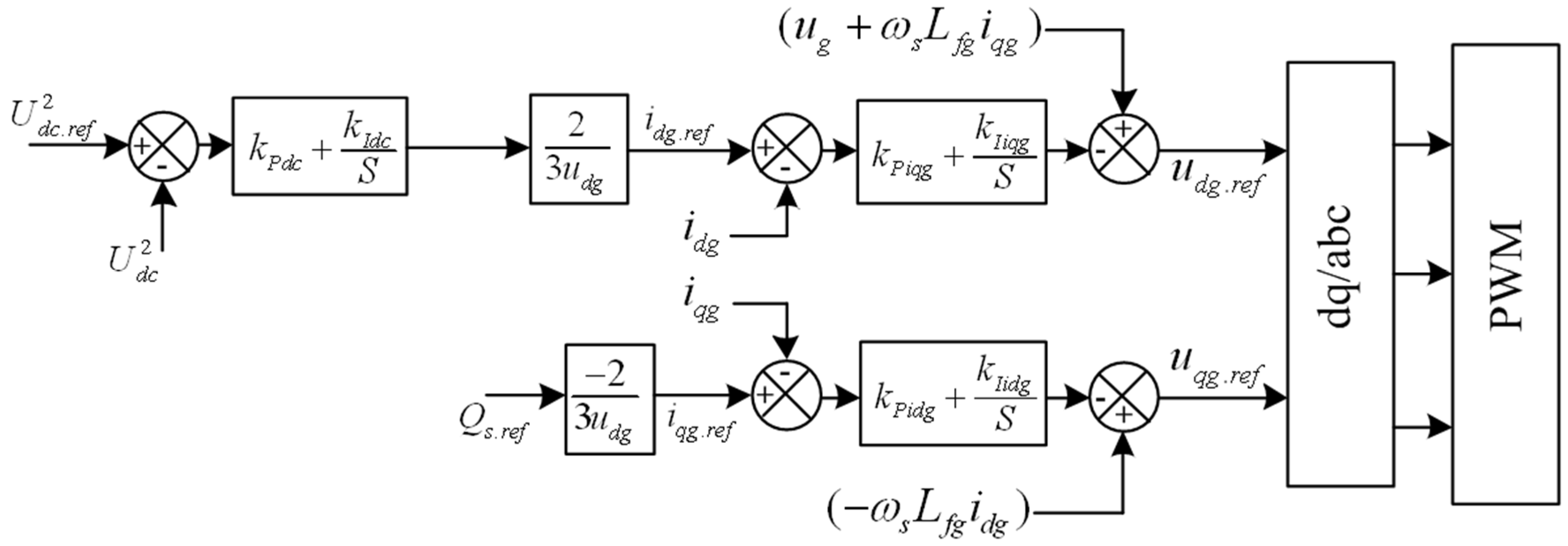
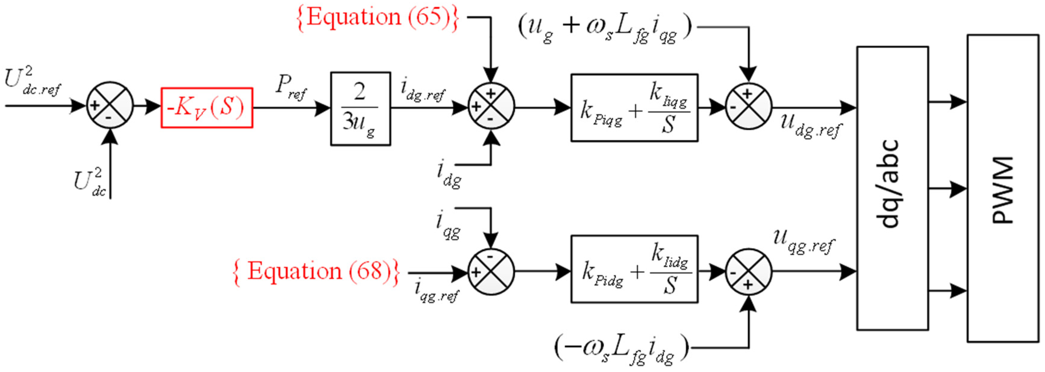
4.2. Control of GSC

The GSC is connected between the DC-link and grid via the grid filter, as shown in Figure 1. The objective is to maintain the DC-link voltage at a given value and regulate the reactive power flow between the GSC and grid.

The conventional control strategy of GSC is implemented in synchronously rotating d-q reference frame with its d-axis oriented with the grid voltage vector based on the vector control technique, as illustrated in Figure 6 [30]. The PI regulators with cascade control loops are used in the GSC control scheme, in which the outer control loop is for the DC-link voltage regulation and the inner control loops are for grid side current regulation.

Figure 6. The conventional control scheme of GSC.

Figure 6. The conventional control scheme of GSC.

Under normal operation conditions, the DC-link voltage is constant because the power flow between the grid and rotor side converters is balanced; this power flow is imbalanced, however, when a voltage dip occurs, so the DC-link voltage may fluctuate. In order to limit the voltage fluctuations in the DC-link, the authors in [18] proposed a control strategy for GSC. However, it ignores the instantaneous absorbed or delivered power in grid side filter. The influences of the interface grid side filter are relatively large with respect to a high power DFIG [20]. This paper proposes a novel control scheme for GSC. The control scheme diagram is illustrated in Figure 7, where two terms have been considered.

Figure 7. The proposed control scheme of GSC.

Figure 7. The proposed control scheme of GSC.

Consideration 1: 

The instantaneous absorbed or delivered power in grid side filter

The voltage equation of the grid filter is:

$$\{\begin{array}{l}{u}_g-u_{df}=R_{fg}{i}_{dg}+L_{fg}\frac{d}{dt}{i}_{dg}-{\mathsf{\omega }}_s{L}_{fg}{i}_{qg}\\ -u_{qf}=R_{fg}{i}_{qg}+L_{fg}\frac{d}{dt}{i}_{qg}+{\mathsf{\omega }}_s{L}_{fg}{i}_{dg}\\ u_{dg}=u_g,u_{qg}=0\end{array}$$

(63)

where R_fg and L_fg are the resistance and inductance of grid side filter, respectively. $u_{df}$, $u_{qf}$, $u_{dg}$ and $u_{qg}$ are the d and q voltage components of grid filter and grid, respectively. $i_{dg}$ and $i_{qg}$ are the d and q current components of the grid filter, respectively.

The dynamic equation of the DC-link can be expressed as [7]:

$$\frac{d}{dt}{U}_{dc}^2=-\frac{2}{C_{dc}}{P}_{rc}-\frac{2}{C_{dc}}{P}_{loss}-\frac{2}{C_{dc}}(P_g+(\frac{2L_{fg}}{3u_{dg}^2})P_g\frac{d{P}_g}{dt}+(\frac{2L_{fg}}{3u_{dg}^2})Q_g\frac{d{Q}_g}{dt})$$

(64)

where $U_{dc}^2$ is the DC-link voltage that represents the output. P_g is the active power at the GSC side that represents the control input. P_loss, P_rc, and Q_g are the loss power in DC-link, active power at the RSC side, and reactive power at the GSC side which represent the disturbance inputs, respectively.

Considering Equation (64), the DC-link voltage oscillates due to the instantaneous absorbed or delivered power in there-phase inductor and the instantaneous imbalance power follow between the RSC and GSC during a grid fault. As shown in Figure 7, The PI regulator of the outer loop is replaced by a compensator K_V(S) that is designed based on an adequately large phase margin under the worst-case operating condition; a more detailed explanation about this design method can be found in [7]. In such a way, the transient performance of the GSC and fluctuation of the DC-link voltage can be improved. Moreover, in order to reduce the voltage fluctuation in the DC-link, the load current feed forward control $i_{RSC}$ is represented as a disturbance to reflect the instantaneous variation of the output power of RSC. The load current can easily be obtained from Equation (65). Thereby, the $i_{dg}$ can be regulated smoothly during a grid fault:

$$i_{RSC}=\frac{P_r}{U_{dc}}=\frac{3}{2}\frac{u_{dr}{i}_{dr}+u_{qr}{i}_{qr}}{U_{dc}}$$

(65)

Consideration 2: 

The maximal voltage value of GSC

When a grid fault is cleared, the voltage in the DC-link increases up to a high value because the grid side voltage exceeds the maximal rated value of the GSC. This value is defined as [7]:

$$u_{\max }(\mathrm{rms})=\frac{\sqrt{3}}{2\sqrt{2}}{U}_{dc}$$

(66)

In order to maintain the DC-link voltage at a given value, the active current must be controlled according to its reference. As shown in Equation (63), the $i_{dg}$ is proportional to $u_{qf}$ during normal operation condition, so $u_{qf}$ should be kept unchanged during a grid fault recovery, $u_{df}$ should be added to:

$$u_{df}=\sqrt{u_{\max }^2(\mathrm{rms})-u_{qf}^2}$$

(67)

Therefore, the reference reactive current should be set to:

$$i_{qg.ref}=\frac{u_{df}-u_g}{{\mathsf{\omega }}_s{L}_{fg}}$$

(68)

5. Case Study and Results

The schematic diagram of the studied system, as shown in Figure 8, including a 2.0 MW-575 V DFIG, WCES, and 50 Hz-20 MVA/25 kV network are built in Power Systems Computer Aided Design (PSCAD). The parameters are listed in the Appendix A1.

Figure 8. The single line diagram for the studied system.

Figure 8. The single line diagram for the studied system.

The transient behaviours of the studied DFIG-WCES are simulated with two different control strategies to demonstrate and compare the effectiveness of the proposed control strategy through the grid fault scenarios based on the FRT requirements as shown in Figure 9 [2]. The two control strategies are:

Figure 9. Fault ride through requirements.

Figure 9. Fault ride through requirements.

Conventional strategy: 

Equip the crowbar and DC-link chopper and use the detailed control scheme that can be found in [34]. The chosen crowbar resistors are all 40 R_r and the protection threshold of rotor and stator currents are both set to 1.5 p.u. The selected DC chopper resistor is 0.5 p.u.and the protection threshold of the DC-link is 1.15 p.u. The control schematic diagram is shown in Figure 3 and Figure 6. The parameters are listed in the Appendix A2.

Proposed strategy: 

The control schematic diagram is analysed in Section 4 and illustrated in Figure 5 and Figure 7. The parameters are listed in the Appendix A2. The following four scenarios have been considered in order to simulate the LVRT capability of the studied DFIG-WCES with two control strategies.

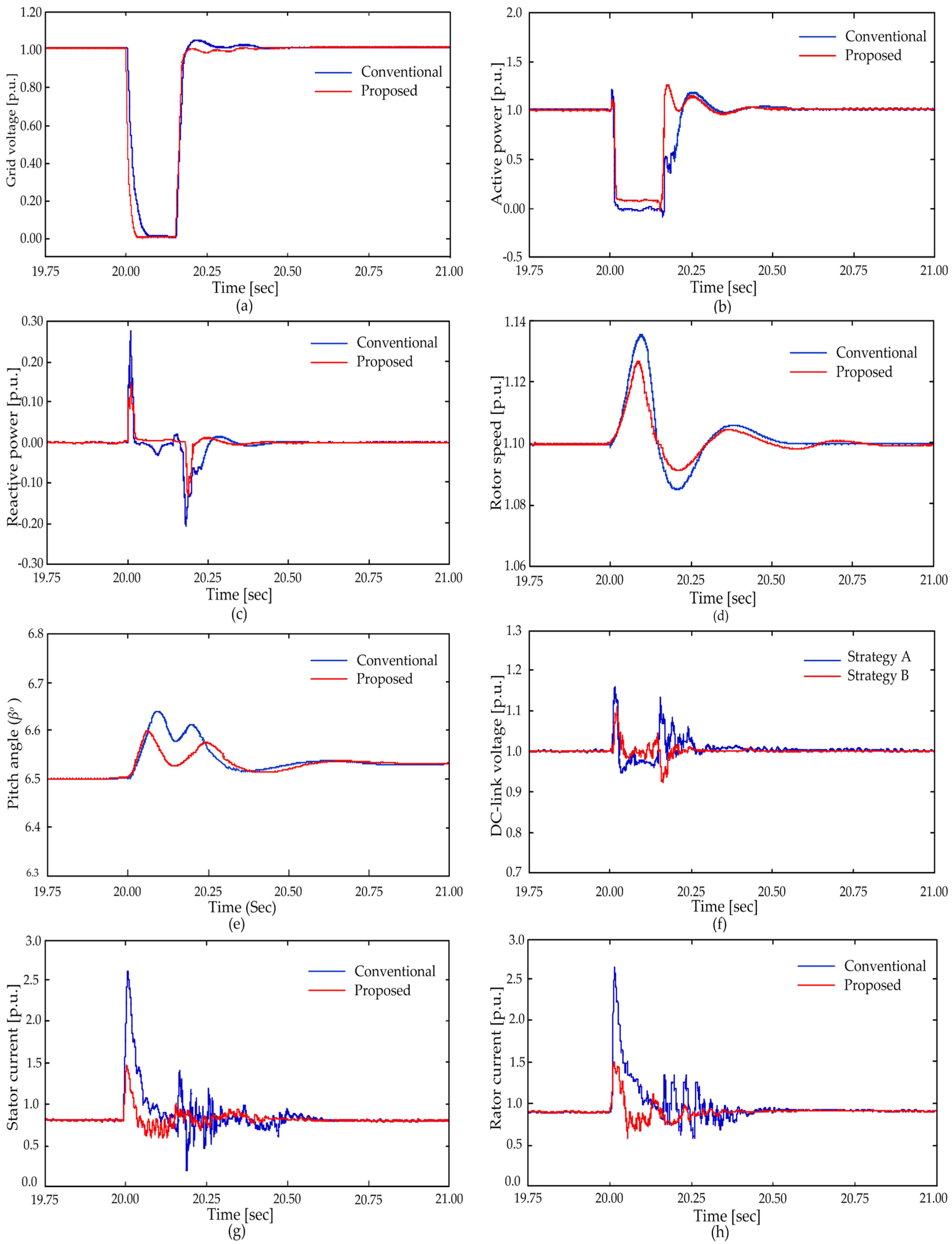
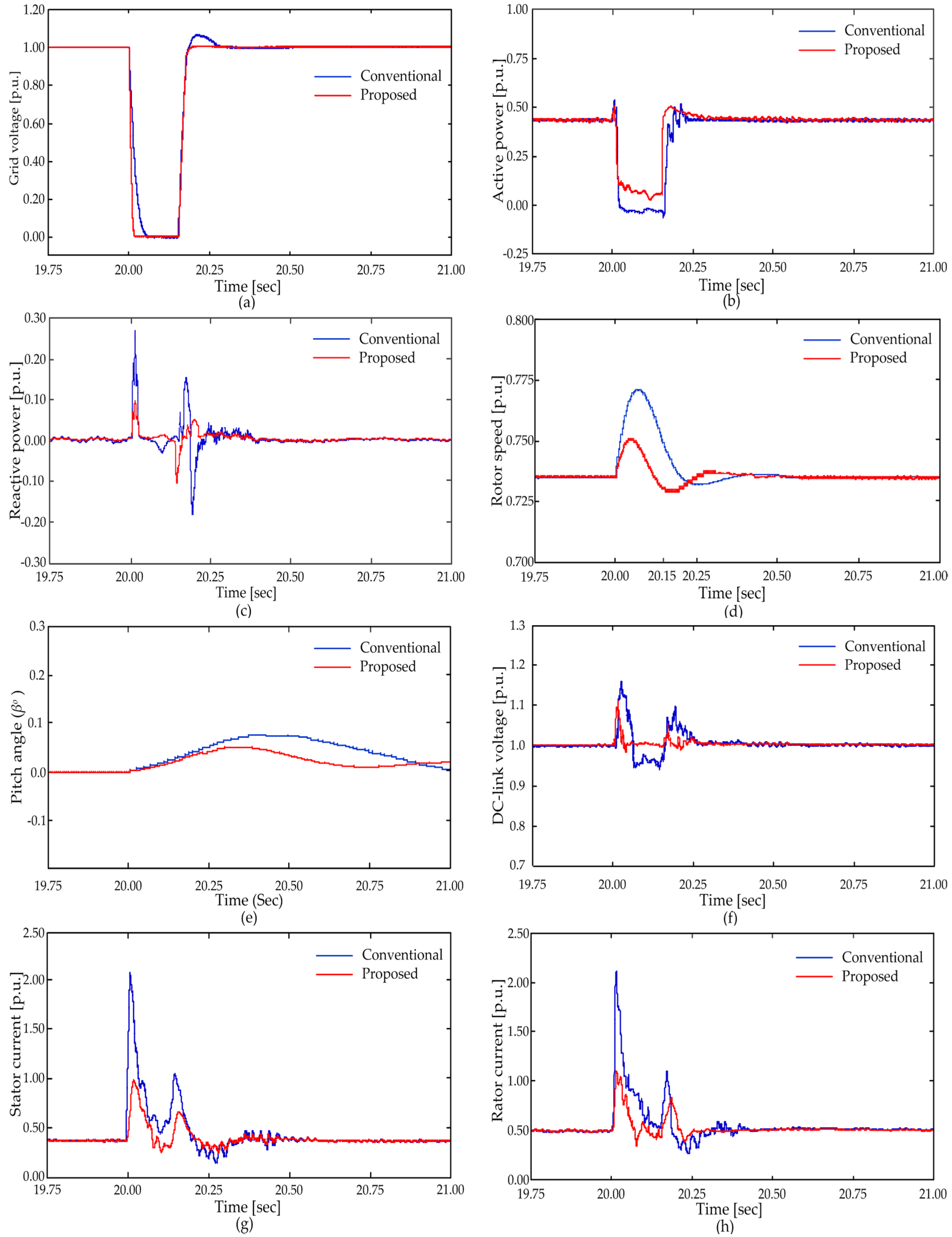
5.1. LVRT Capability under Symmetrical Fault Scenarios

In this subsection, a three-phase short-circuit fault are simulated to show the ride through symmetrical low voltage fault behaviors of DFIG-WCES.

First Scenario: 

At time t = 20 s, a three-phase short-circuit fault occurs at point A on the transmission line, as shown Figure 8. During the fault, the voltage at PCC dips to zero with a duration 0.15 s. The DFIG-WCES is operating at wind speed of 8 m/s, this wind speed value corresponds to the hypo-synchronous operation mode of the DFIG.

Figure 10 shows the dynamic responses of the investigated system. Once the fault is detected, the stator active power P_s = (3/2)(L_m/L_s)u_si_qr is decreased due to the stator voltage dip. As a result, the exchanged active power with the grid is decreased, as identified Figure 10b. The reactive power Q_s = (3/2)u_s((L_m/L_s)i_dr–(u_s/ω_s/L_s)) is normally equal to zero, that is to say ((L_m/L_s)i_dr–(u_s/ω_s/L_s)) is equal to zero, when the stator voltage dip occurs, the reactive power Q_s is increased because the component of ((L_m/L_s)i_dr–(u_s/ω_s/L_s)) is increased from zero, so that the exchanged reactive power with the grid (Q_gen) is increased, as shown in Figure 10c. The generator rotor speed is increased because the inertia of the generator-turbine system is very large, as evident in Figure 10d. Figure 10g,h show, the currents in the rotor and stator circuits are increased because the stator currents appear the DC-components; these currents appear as AC-components in the rotor side. Figure 10e shows that the pitch angle is activated to stabilize the operation of the system. In addition, Figure 10f shows the DC-link voltage rises instantaneously because of the rotor inrush currents injected from the RSC into the DC-link capacitor.

Therefore, by using the proposed control strategy, which has been analyzed in Section 4, the transient responses of the active and reactive power, DC-link voltage, rotor speed, rotor and stator currents, and pitch angle are significantly improved more than with a conventional one during the fault duration. This conclusion is deduced based on the simulation results that are summarized as follows: the acceleration of the rotor speed is fast and its oscillations are attenuated. The exchanged active power into the grid is 0.05 p.u. of 0.44 p.u. and the oscillations are well cleared. The exchanged reactive power decreases back to zero and the oscillations are well cleared. The DC-link voltage does not exceed above the 1.115 p.u., which is less than the activation threshold of the protective DC-chopper. In addition, the stator and rotor currents do not exceed above the 0.98 and 1.11 p.u., respectively, which are less than the activation threshold of the protective crowbar.

Second Scenario: 

In this case, the scenario has been performed the same as first scenario, considering the operating DFIG-WCES at wind speed 13 m/s, this wind value corresponds to the hyper-synchronous operation mode of machine. In this paper, the rated wind speed of the studied DFIG-WCES is 12 m/s, this wind value corresponds to the synchronous operation mode of the machine.

Figure 10. Dynamic responses of the 2.0 MW DFIG-WCES under first scenario: (a) voltage at the terminal; (b) active power to the grid; (c) reactive power to the grid; (d) generator rotor speed; (e) pitch angle; (f) DC-link voltage; (g) stator current; (h) rotor current.

Figure 10. Dynamic responses of the 2.0 MW DFIG-WCES under first scenario: (a) voltage at the terminal; (b) active power to the grid; (c) reactive power to the grid; (d) generator rotor speed; (e) pitch angle; (f) DC-link voltage; (g) stator current; (h) rotor current.

Figure 11d,e show that when the wind speed is 13 m/s, which is higher than the rated wind speed, leading to the over-speed of WT, the pitch controller is immediately activated to keep the rotor speed at 1.1 p.u., corresponding to the pitch angle at 6.52 degrees; whereas the pitch angle is equal zero in the case of the low wind speed, as shown Figure 10d. As a result, the transformation of the electric energy into the kinetic energy can be limited. Therefore, the DC-link voltage and the rotor speed during the fault are smaller than the first scenario.

Figure 11. Dynamic responses of the 2.0 MW DFIG-WCES under second scenario: (a) voltage at the terminal; (b) active power to the grid; (c) reactive power to the grid; (d) generator rotor speed; (e) pitch angle; (f) DC-link voltage; (g) stator current; (h) rotor current.

Figure 11. Dynamic responses of the 2.0 MW DFIG-WCES under second scenario: (a) voltage at the terminal; (b) active power to the grid; (c) reactive power to the grid; (d) generator rotor speed; (e) pitch angle; (f) DC-link voltage; (g) stator current; (h) rotor current.

Figure 11 shows that the LVRT behaviours of the DC-link voltage, the rotor speed, the active and reactive power, stator and rotor currents, and pitch angle by using the proposed control strategy are still observed to be better than with the conventional one. Specifically, the proposed control strategy can intercept the transient DC-link voltage and rotor and stator currents slower than the DC-chopper and crowbar protection threshold; thus, the DFIG-WECS can maintain uninterrupted control of reactive and active power.

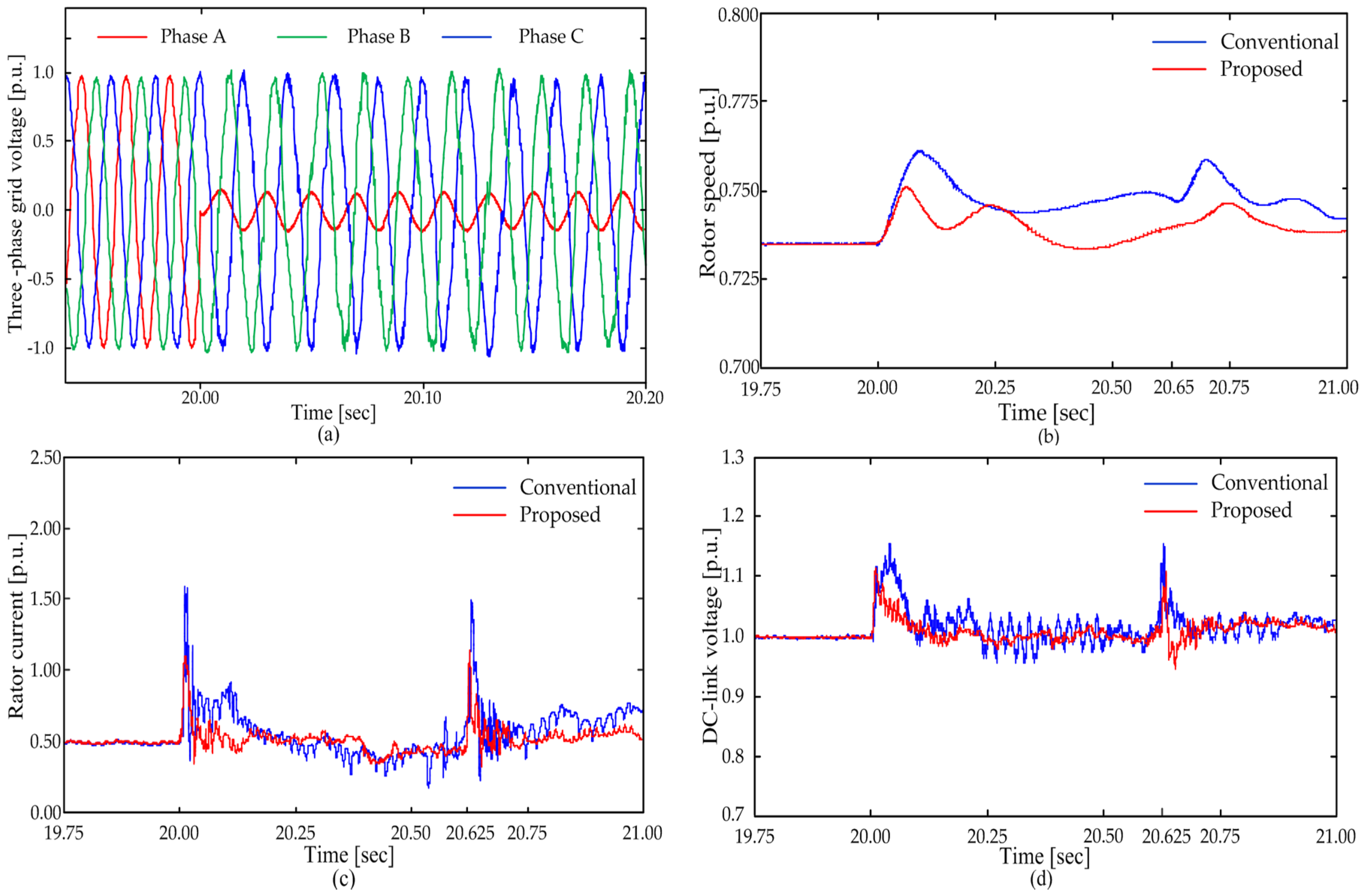
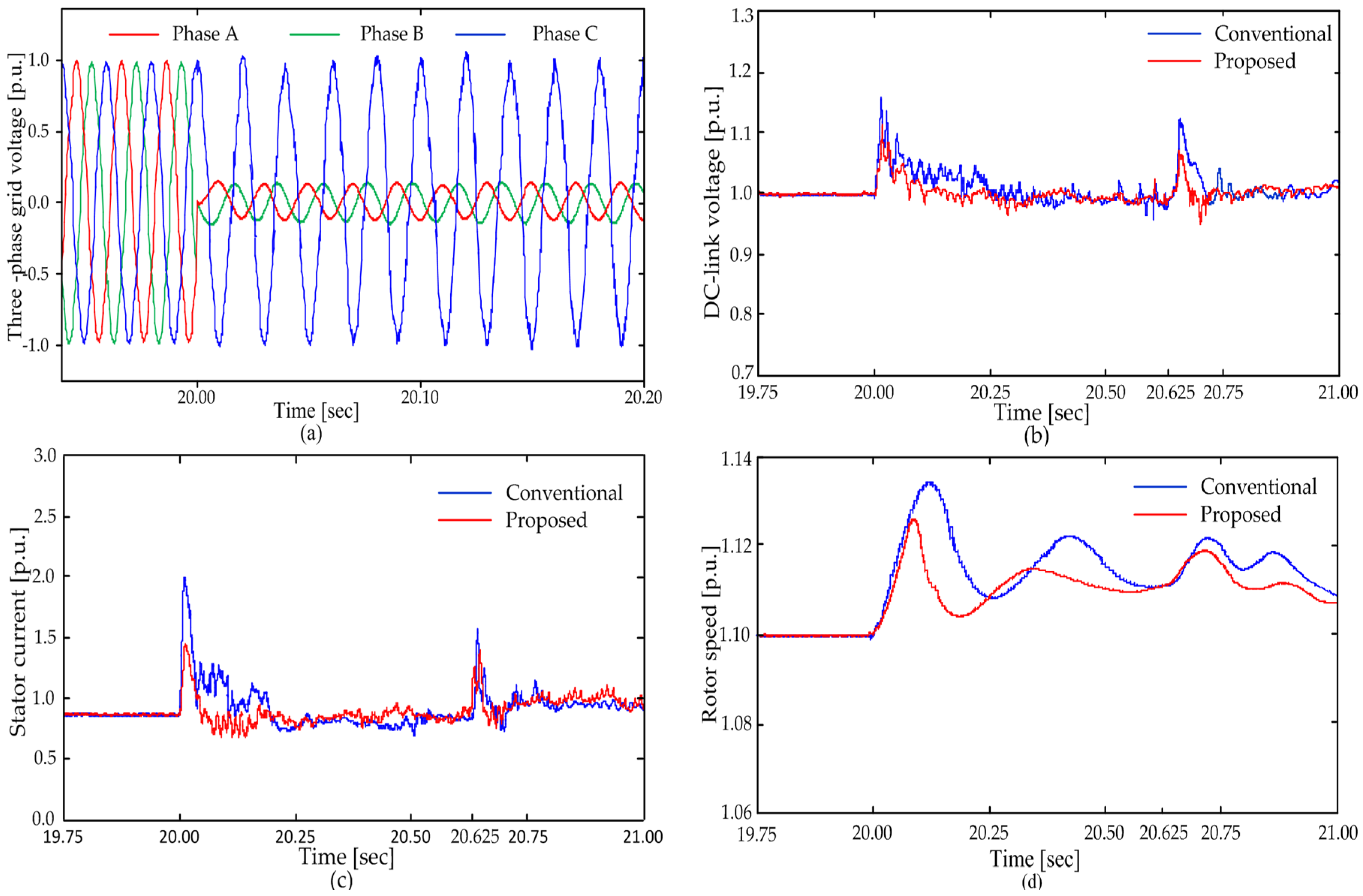
5.2. LVRT Capability under Asymmetrical Fault Scenarios

As substantiated in Section 5.1, a three-phase short circuit fault is considered as the worst case, though it is symmetrical and not as frequent as other faults. For example, the one- and two-phase short-circuit faults are interesting cases because they occur relatively often and present asymmetry. In this subsection, the one- and two-phase-to-ground short-circuit faults are simulated to show the ride-through asymmetrical low voltage fault behaviors of the studied DFIG-WCES.

Third Scenario: 

Figure 12a shows a one-phase-to-ground voltage dip simulated for the system, in which the grid voltage in phases A drops to 0.15 p.u at time t = 20 s, with a duration 0.625 s. The DFIG-WCES is operating at a wind speed of 8 m/s, this wind speed value corresponds to the hypo-synchronous operation mode of the DFIG. Figure 12b–d show, that by applying the proposed control strategy, the LVRT capability of the DFIG-WCES can be improved in terms of both the peak values and oscillations damping of transient response.

Figure 12. Dynamic responses of the 2.0 MW DFIG-WCES under third scenario: (a) There-phase grid voltage; (b) Rotor speed; (c) Rotor current; (d) DC-link voltage.

Figure 12. Dynamic responses of the 2.0 MW DFIG-WCES under third scenario: (a) There-phase grid voltage; (b) Rotor speed; (c) Rotor current; (d) DC-link voltage.

Fourth scenario: 

Figure 13a shows the system is simulated for a two-phase-to-ground voltage dip, in which the grid voltage in phases A and B drops to 0.15 p.u at time t = 20 s and lasts 0.625 s. The DFIG-WCES is operating at wind speed of 13 m/s. It can be shown in Figure 13b–d, with the proposed control strategy, the DFIG-WCES is operating at high wind speed can remain connected to the grid during a two-phase-to-ground fault with a longer time. In Figure 13d, the rotor speed is increased only slightly because the system inertia is very large. However, the operating speed before the fault is 1.1 p.u. and the maximum generator speed during the fault is 1.135 p.u, so that the generator slips during and after the fault are within the allowable range. In addition, the growth of the generator speed during the grid fault is relatively low. Therefore, The DFIG-WCES does not face instability. In summary, Figure 12 and Figure 13 show clearly that the DFIG-WCES can ride through the asymmetrical fault successfully by the proposed method.

Figure 13. Dynamic responses of the 2.0 MW DFIG-WCES under fourth scenario: (a) There-phase grid voltage; (b) DC-link voltage; (c) Stator current; (d) Rotor speed.

Figure 13. Dynamic responses of the 2.0 MW DFIG-WCES under fourth scenario: (a) There-phase grid voltage; (b) DC-link voltage; (c) Stator current; (d) Rotor speed.

6. Conclusions

In this paper, a novel and efficient control strategy for both the rotor and grid side converters which makes full use of existing properties within the generator-turbine system without using any extra protective hardware, is proposed to enhance the low voltage ride-through fault (LVRT) capability of the DFIG-WCES. The proposed control strategy and the conventional one that is equipped with protective crowbar and DC-link chopper are examined through the simulation of a 2.0 MW-575 V DFIG-WECS. Based on the obtained results under transient conditions, the amplitudes of oscillation of the active and reactive power, rotor and stator currents, DC-link voltage, etc. are significantly reduced when the proposed control strategy is employed. Furthermore, the oscillations are dampened out faster, and the DFIG-WCES reaches its steady state in a shorter time. Thus, the LVRT capability of DFIG is significantly improved and has enough ability to continue the electricity supply into the network.

References

- The Global Wind Report Annual Market Update 2014. Available online: http://www.gwec.net (accessed on 8 March 2015).
- Tsili, M.; Papathanassiou, S. A review of grid code technical requirements for wind farms. IET Renew. Power Gener. 2009, 3, 308–332. [Google Scholar] [CrossRef]
- Anca, D.H. Wind Power in Power Systems, 2nd ed.; Ackermann, T., Ed.; John Wiley & Sons: Chichester, West Sussex, UK, 2012; pp. 73–102. [Google Scholar]
- Boukhezzar, B.; Siguerdidjane, H. Nonlinear control with wind estimation of a DFIG variable speed wind turbine for power capture optimization. Energy Convers. Manag. 2009, 50, 885–892. [Google Scholar] [CrossRef]
- Fernandez, L.M.; Garcia, C.A.; Saenz, J.R.; Jurado, F. Equivalent models of wind farms by using aggregated wind turbines and equivalent winds. Energy Convers. Manag. 2009, 50, 691–704. [Google Scholar] [CrossRef]
- Müller, S.; Deicke, M.; de Doncker, R.W. Doubly fed induction generator systems for wind turbines. IEEE Ind. Appl. Mag. 2002, 8, 26–33. [Google Scholar] [CrossRef]
- Yazdani, A.; Iravani, R. Voltage-Sourced Converters in Power Systems: Modeling, Control, and Applications; John Wiley & Sons: Hoboken, NJ, USA, 2010; pp. 127–310. [Google Scholar]
- Seman, S.; Niiranen, J.; Arkkio, A. Ride-through analysis of doubly fed induction wind-power generator under unsymmetrical network disturbance. IEEE Trans. Power Syst. 2006, 21, 1782–1789. [Google Scholar] [CrossRef]
- Rahimi, M.; Parniani, M. Grid-fault ride-through analysis and control of wind turbines with doubly fed induction generators. Electr. Power Syst. Res. 2010, 80, 184–195. [Google Scholar] [CrossRef]
- Okedu, K.E.; Muyeen, S.M.; Takahashi, R.; Tamura, J. Wind farms fault ride through using DFIG with new protection scheme. IEEE Trans. Sustain. Energy 2012, 3, 242–254. [Google Scholar] [CrossRef]
- Yao, J.; Li, Q.; Chen, Z.; Liu, A. Coordinated control of a DFIG-based wind-power generation system with SGSC under distorted grid voltage conditions. Energies 2013, 6, 2541–2561. [Google Scholar] [CrossRef]
- Flannery, P.S.; Venkataramanan, G. A fault tolerant doubly fed induction generator wind turbine using a parallel grid side rectifier and series grid side converter. IEEE Trans. Power Electron. 2008, 23, 1126–1135. [Google Scholar] [CrossRef]
- Yao, J.; Li, H.; Chen, Z.; Xia, X.; Chen, X.; Li, Q.; Liao, Y. Enhanced control of a DFIG-based wind-power generation system with series grid-side converter under unbalanced grid voltage conditions. IEEE Trans. Power Electron. 2013, 28, 3167–3181. [Google Scholar] [CrossRef]
- Wessels, C.; Gebhardt, F.; Fuchs, F.W. Fault ride-through of a DFIG wind turbine using a dynamic voltage restorer during symmetrical and asymmetrical grid faults. IEEE Trans. Power Electron. 2011, 26, 807–815. [Google Scholar] [CrossRef]
- Ibrahim, A.O.; Nguyen, T.H.; Lee, D.C.; Kim, S.C. A fault ride-through technique of DFIG wind turbine systems using dynamic voltage restorers. IEEE Trans. Power Syst. 2011, 26, 871–882. [Google Scholar] [CrossRef]
- Qiao, W.; Harley, R.G.; Venayagamoorthy, G.K. Coordinated reactive power control of a large wind farm and a STATCOM using heuristic dynamic programming. IEEE Trans. Energy Convers. 2009, 24, 493–503. [Google Scholar] [CrossRef]
- Hu, S.; Lin, X.; Kang, Y.; Zou, X. An improved low-voltage ride-through control strategy of doubly fed induction generator during grid faults. IEEE Trans. Power Electron. 2011, 26, 3653–3665. [Google Scholar] [CrossRef]
- Yang, L.; Xu, Z.; Østergaard, J.; Dong, Z.Y.; Wong, K.P. Advanced control strategy of DFIG wind turbines for power system fault ride through. IEEE Trans. Power Syst. 2012, 27, 713–722. [Google Scholar] [CrossRef]
- Xie, D.; Xu, Z.; Yang, L.; Ostergaard, J.; Xue, Y.; Wong, K.P. A comprehensive LVRT control strategy for DFIG wind turbines with enhanced reactive power support. IEEE Trans. Power Syst. 2013, 28, 3302–3310. [Google Scholar] [CrossRef]
- Rahimi, M.; Parniani, M. Coordinated control approaches for low-voltage ride-through enhancement in wind turbines with doubly fed induction generators. IEEE Trans. Energy Convers. 2008, 25, 873–883. [Google Scholar] [CrossRef]
- Abad, G.; Lopez, J.; Rodríguez, M.; Marroyo, L.; Iwanski, G. Doubly Fed Induction Machine: Modeling and Control for Wind Energy Generation; Hanzo, L., Ed.; John Wiley & Sons: Hoboken, NJ, USA, 2011; pp. 265–301. [Google Scholar]
- Quang, N.P.; Dittrich, J.A. Vector Control of Three-Phase AC Machines; Springer: Berlin/Heidelberg, Germany, 2008; pp. 185–223. [Google Scholar]
- Wu, B.; Lang, Y.; Zargari, N.; Kouro, S. Power Conversion and Control of Wind Energy System; Hanzo, L., Ed.; John Wiley & Sons: Hoboken, NJ, USA, 2011; pp. 49–85. [Google Scholar]
- Fan, L.; Kavasseri, R.; Miao, Z.L.; Zhu, C. Modeling of DFIG-based wind farms for SSR analysis. IEEE Trans. Power Deliv. 2010, 25, 2073–2082. [Google Scholar] [CrossRef]
- Iov, F.; Hansen, A.D.; Sorensen, P.; Blaabjerg, F. Wind Turbine Blockset in Matlab/Simulink; Aalborg University: Aalborg, Denmark, 2004; pp. 21–87. [Google Scholar]
- Zhang, W.; Xu, Y.; Liu, W.; Ferrese, F.; Liu, L. Fully distributed coordination of multiple DFIGs in a microgrid for load sharing. IEEE Trans. Smart Grid 2013, 4, 806–815. [Google Scholar] [CrossRef]
- Miller, N.W.; Price, W.W.; Sanchez-Gasca, J.J. Dynamic Modeling of GE 1.5 and 3.6 Wind Turbine-Generators; General Electric International, Power Systems Energy Consulting: Schenectady, NY, USA, 2003. [Google Scholar]
- Abad, G.; Rodriguez, M.A.; Poza, J.; Canales, J.M. Direct torque control for doubly fed induction machine-based wind turbines under voltage dips and without crowbar protection. IEEE Trans. Energy Convers. 2010, 25, 586–588. [Google Scholar] [CrossRef]
- Xu, L.; Wang, Y. Dynamic modeling and control of DFIG-based wind turbines under unbalanced network conditions. IEEE Trans. Power Syst. 2007, 22, 314–323. [Google Scholar] [CrossRef]
- Pena, R.; Clare, J.C.; Asher, G.M. Doubly fed induction generator using back-to-back PWM converters and its application to variable-speed wind-energy generation. IEEE Proc. Electr. Power Appl. 1996, 143, 231–241. [Google Scholar] [CrossRef]
- Ortega, R.; Loría, A.; Nicklasson, P.J.; Sira-Ramírez, H. Passivity-Based Control of Euler-Lagrange Systems: Mechanical, Electrical and Electromechanical Applications; Springer-Verlag: Berlin, Germany, 1998; pp. 133–510. [Google Scholar]
- Belabbes, B.; Lousdad, A.; Meroufel, A.; Larbaoui, A. Simulation and Modelling of Passivity Based Control of PMSM Under Controlled Voltage. J. Electr. Eng. 2013, 64, 298–304. [Google Scholar] [CrossRef]
- Aïssi, S. Contribution au Contrôle de la Machine Asynchrone Double Alimentée. Ph.D. Thesis, University of Batna, Batna, Algeria, 2010. [Google Scholar]
- Wang, Y.; Wu, Q.; Xu, H.; Guo, Q.; Sun, H. Fast coordinated control of DFIG wind turbine generators for low and high voltage ride-through. Energies 2014, 7, 4140–4156. [Google Scholar] [CrossRef] [Green Version]
© 2016 by the authors; licensee MDPI, Basel, Switzerland. This article is an open access article distributed under the terms and conditions of the Creative Commons by Attribution (CC-BY) license (http://creativecommons.org/licenses/by/4.0/).
Share and Cite
Le, V.; Li, X.; Li, Y.; Dong, T.L.T.; Le, C. An Innovative Control Strategy to Improve the Fault Ride-Through Capability of DFIGs Based on Wind Energy Conversion Systems. Energies 2016, 9, 69. https://doi.org/10.3390/en9020069
Le V, Li X, Li Y, Dong TLT, Le C. An Innovative Control Strategy to Improve the Fault Ride-Through Capability of DFIGs Based on Wind Energy Conversion Systems. Energies. 2016; 9(2):69. https://doi.org/10.3390/en9020069
Chicago/Turabian StyleLe, Vandai, Xinran Li, Yong Li, Tran Le Thang Dong, and Caoquyen Le. 2016. "An Innovative Control Strategy to Improve the Fault Ride-Through Capability of DFIGs Based on Wind Energy Conversion Systems" Energies 9, no. 2: 69. https://doi.org/10.3390/en9020069