
A New Fluctuation Index: Characteristics and Application to Hydro-Wind Systems


Abstract
:1. Introduction
2. Methods and Materials
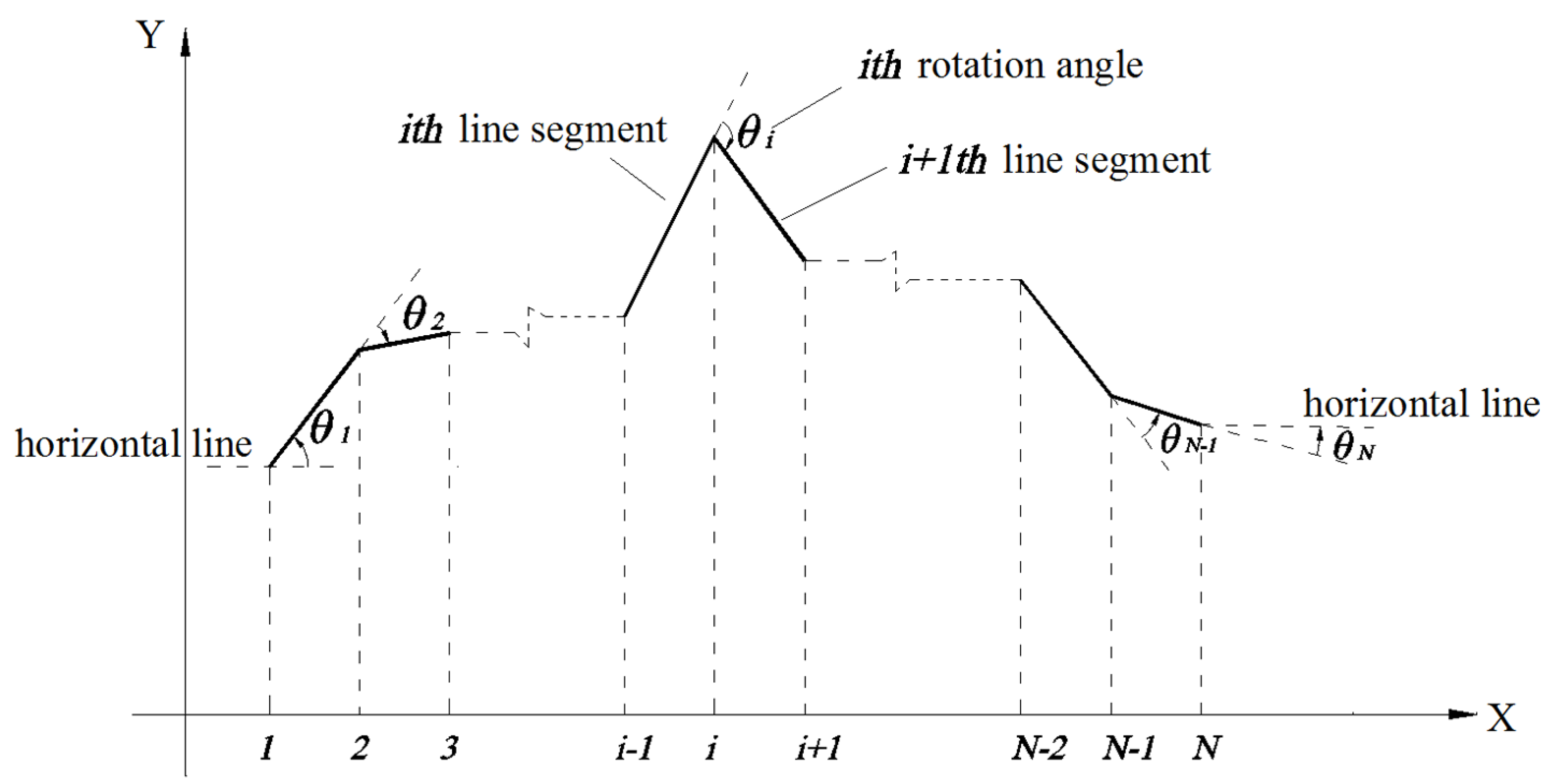
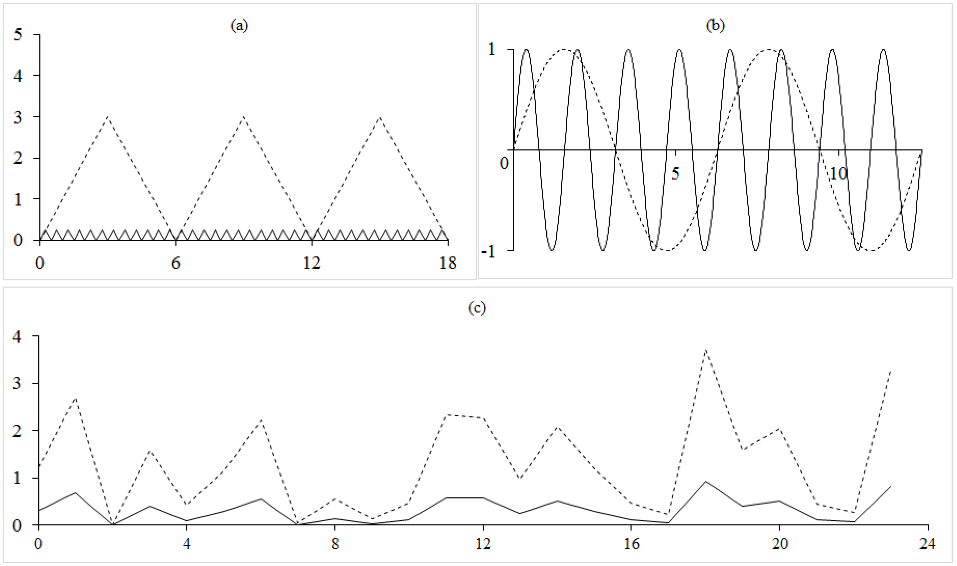
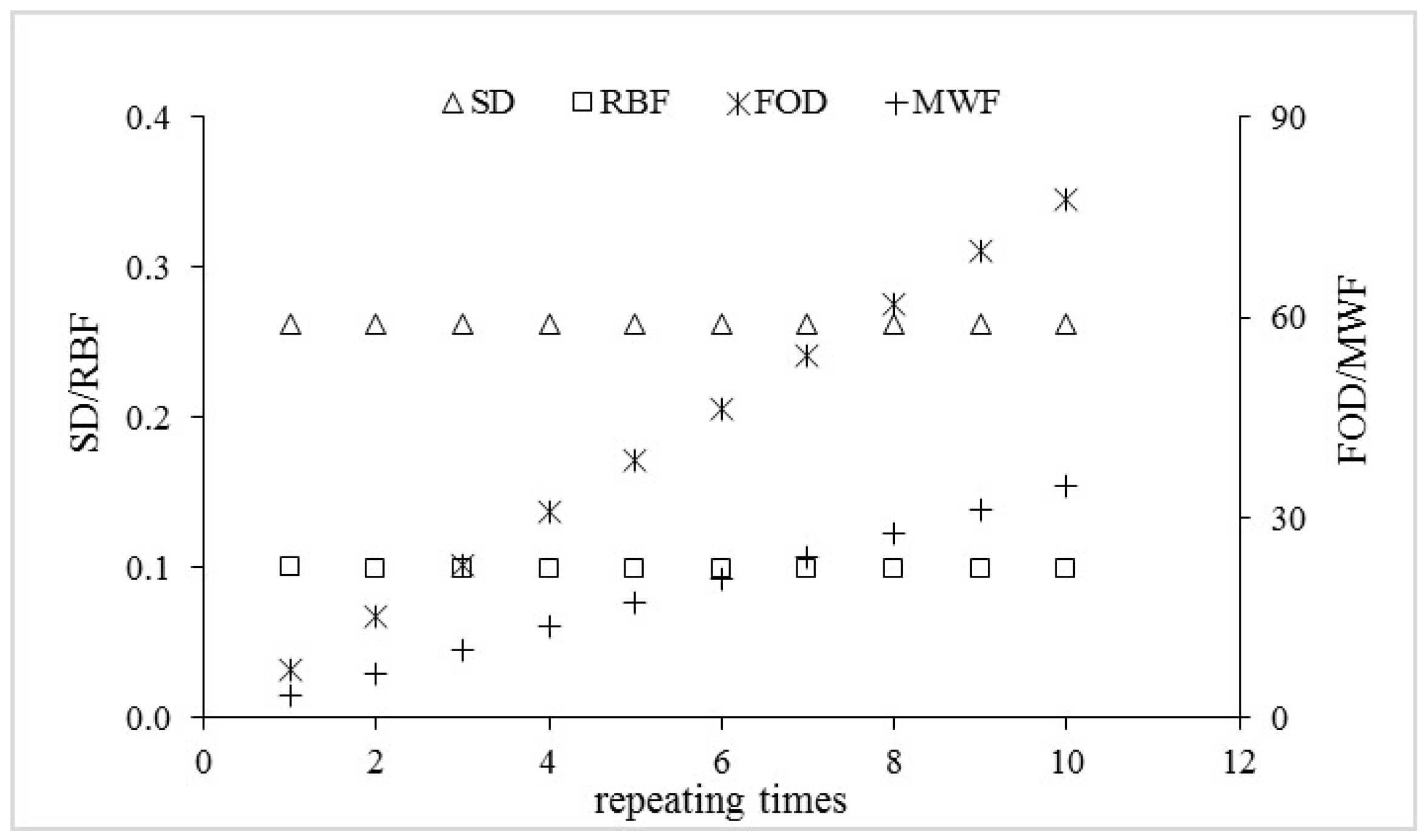
2.1. Methods
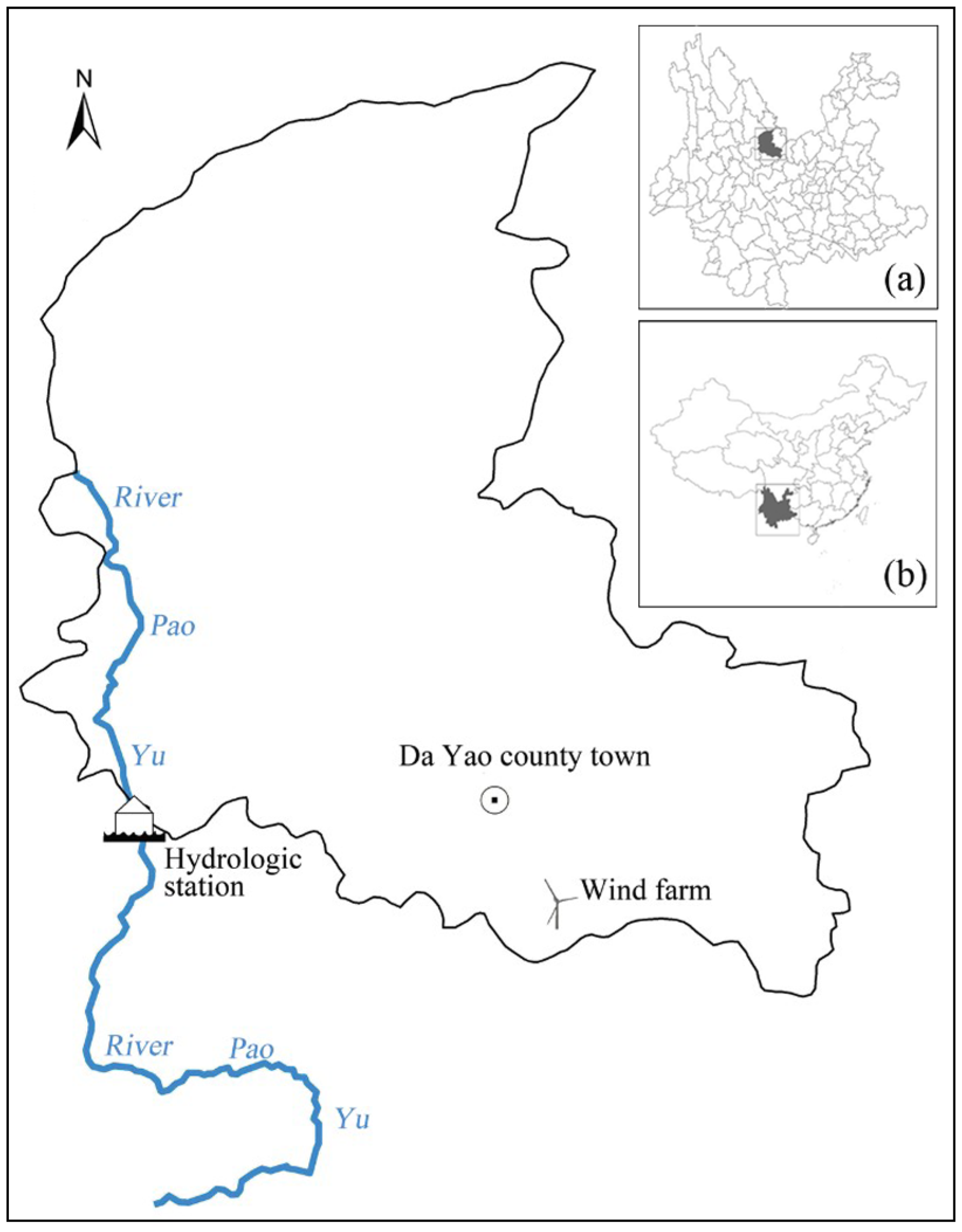
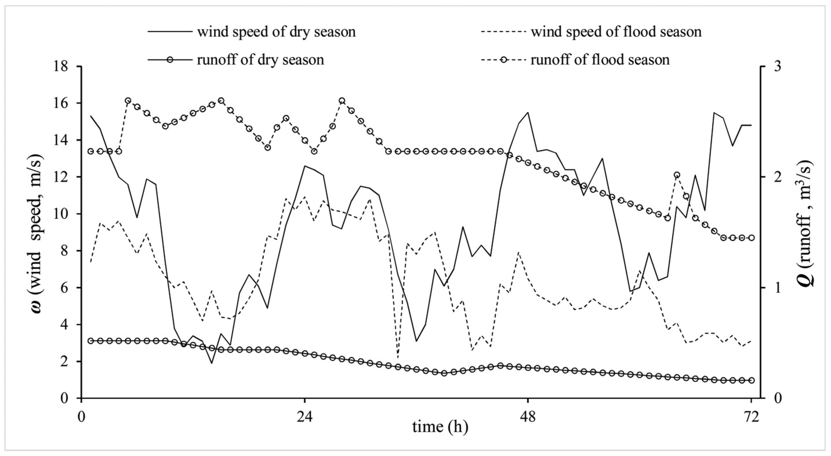
2.2. Materials
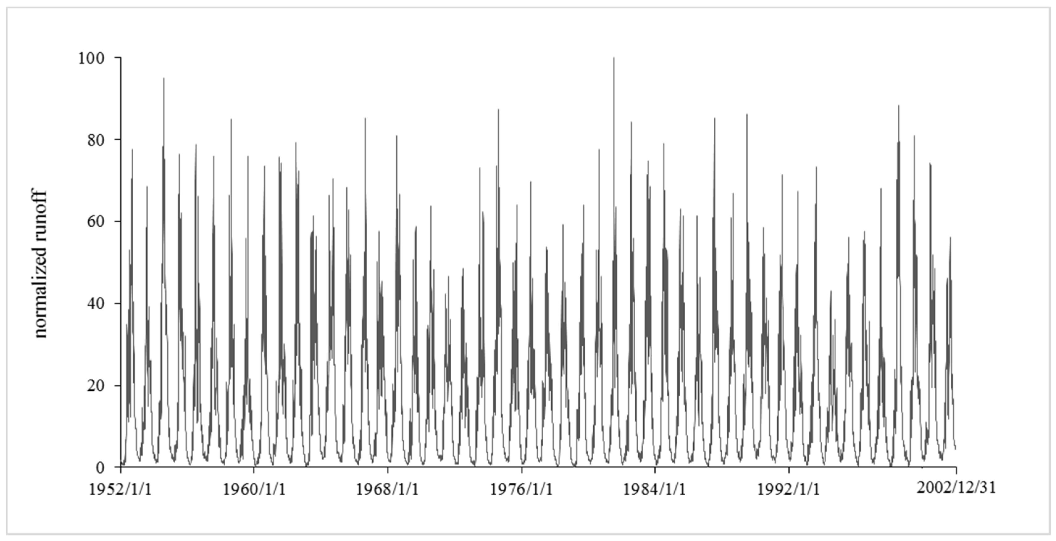
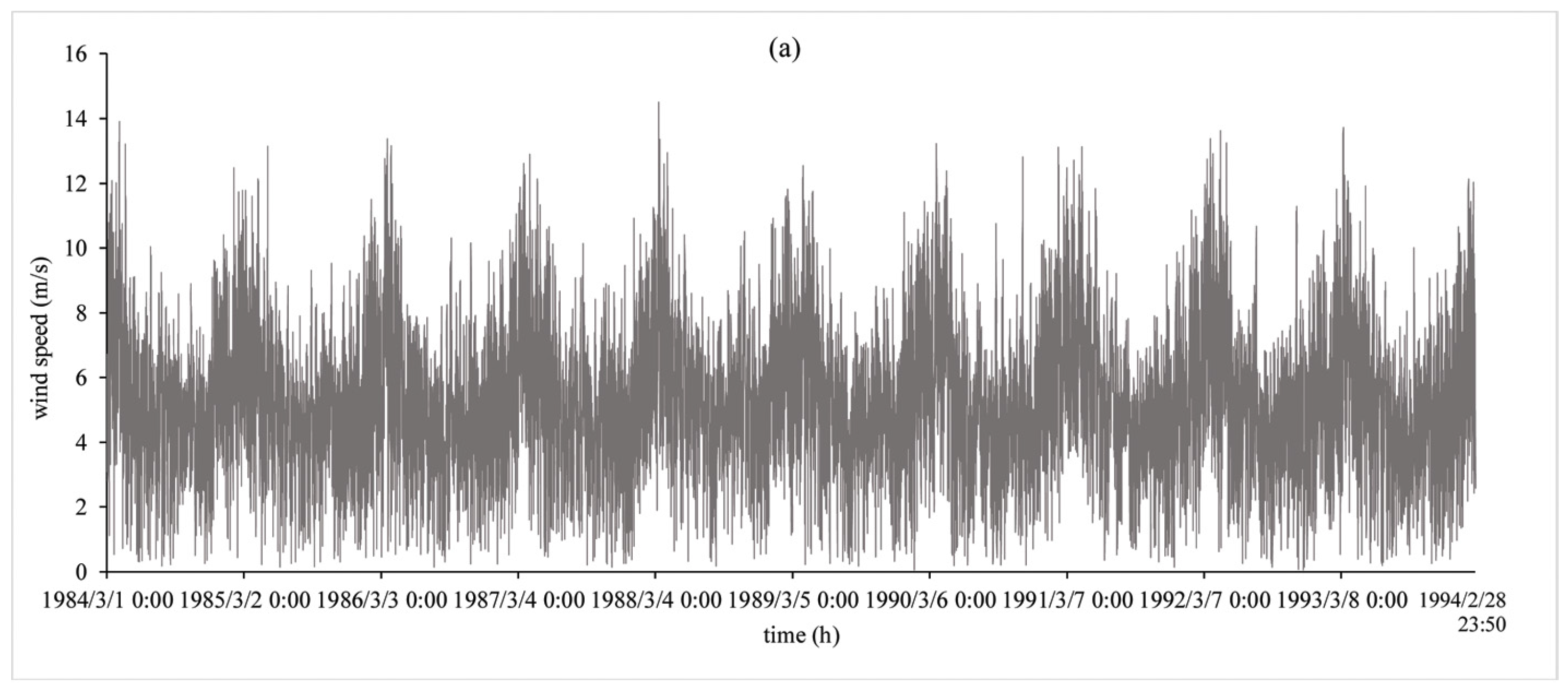
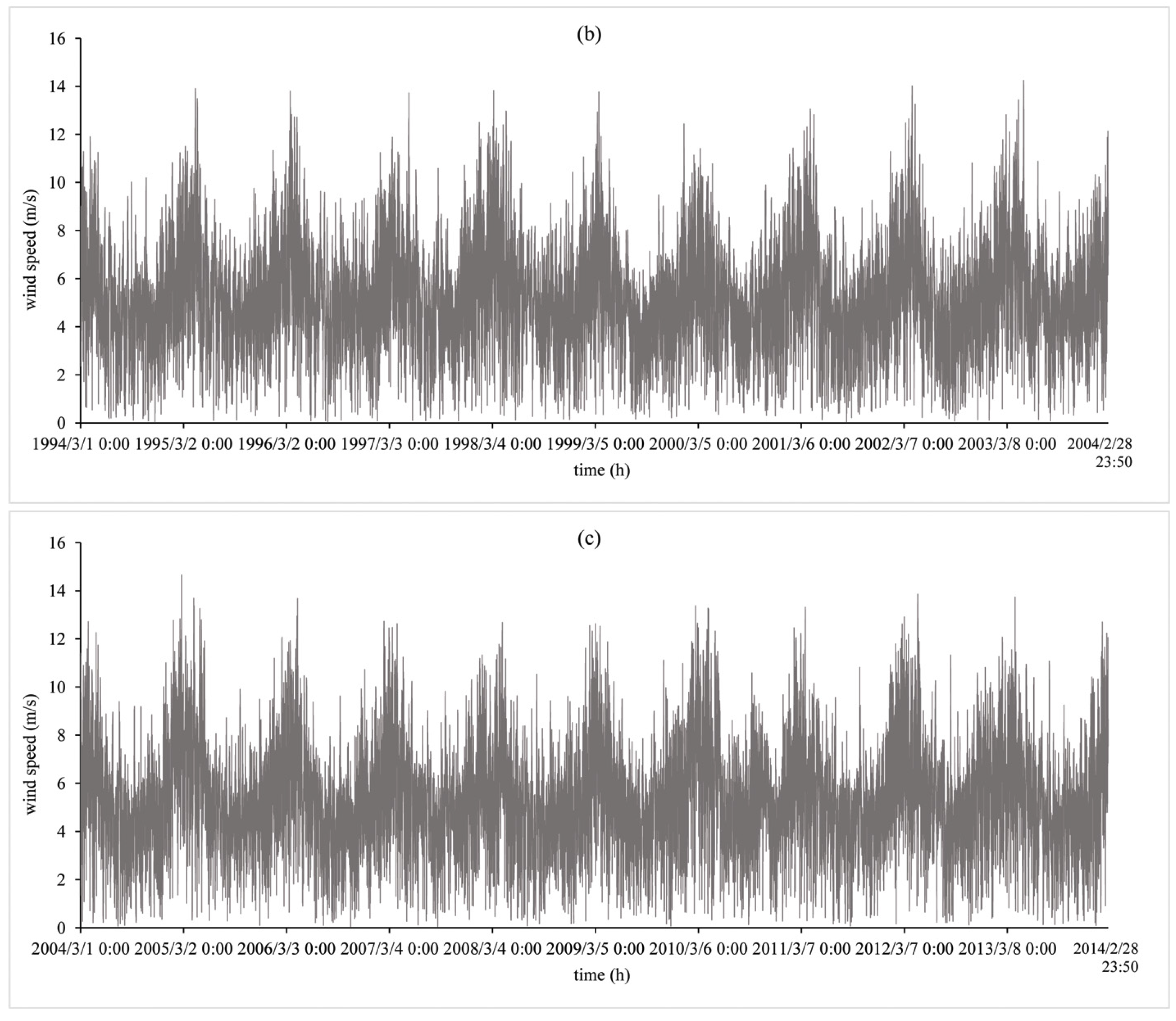
2.2.1. Process
2.2.2. Combined Hydro-Wind Power System
3. Results and Discussion
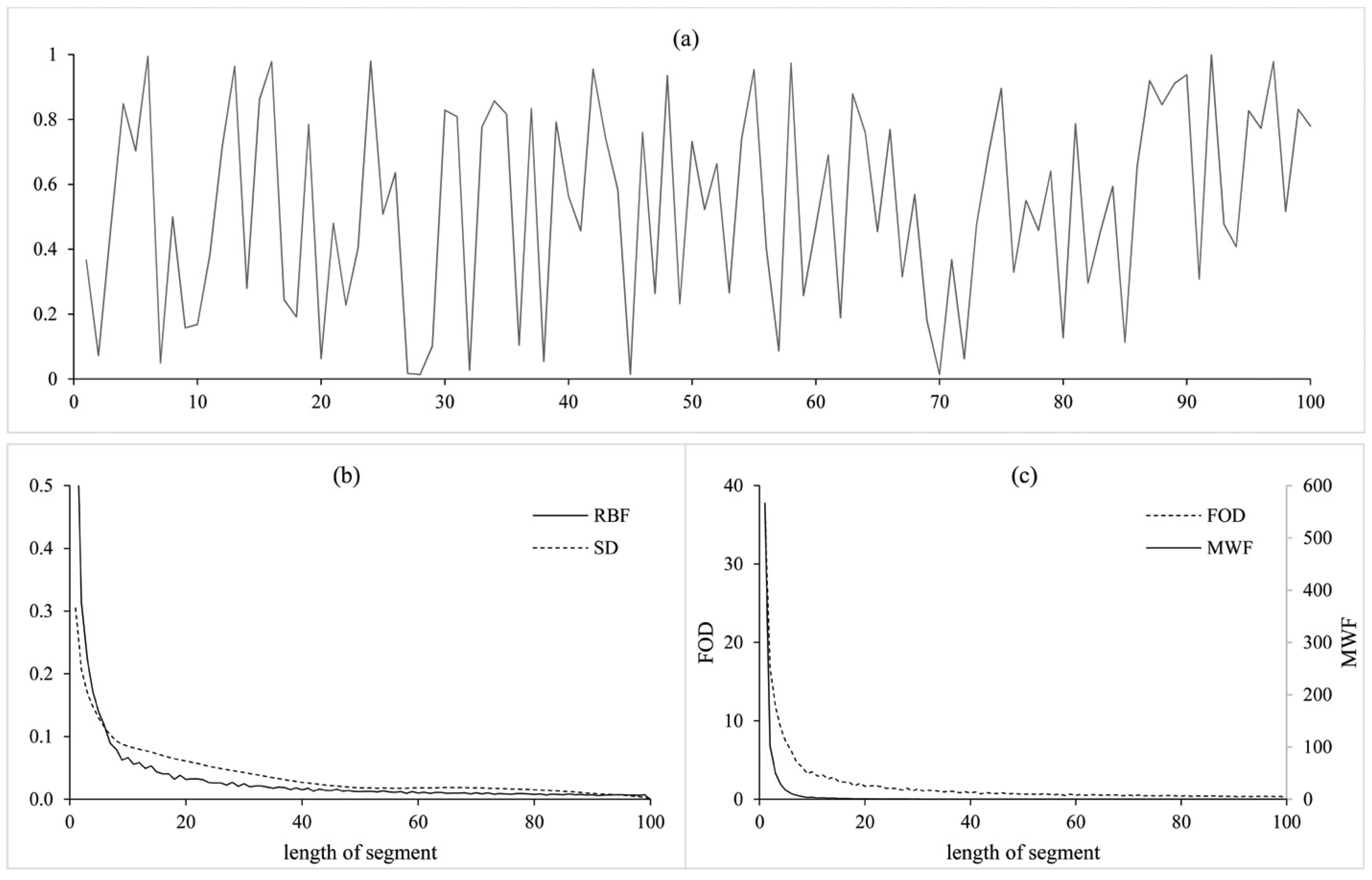
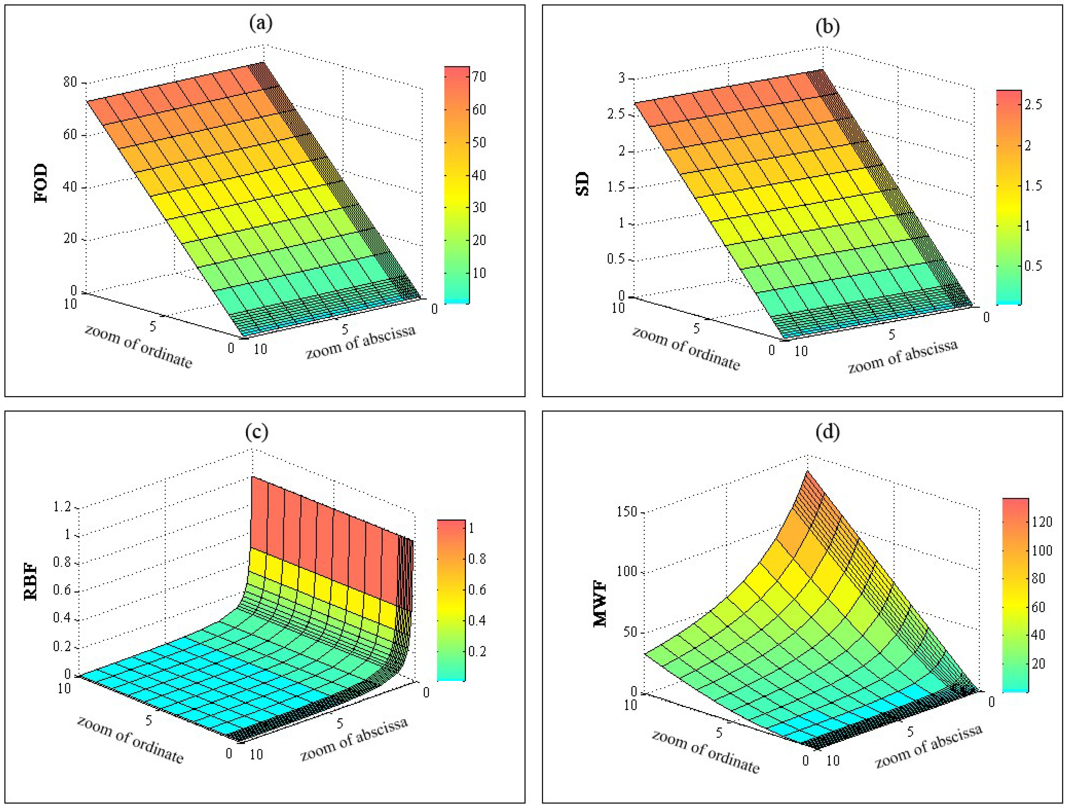
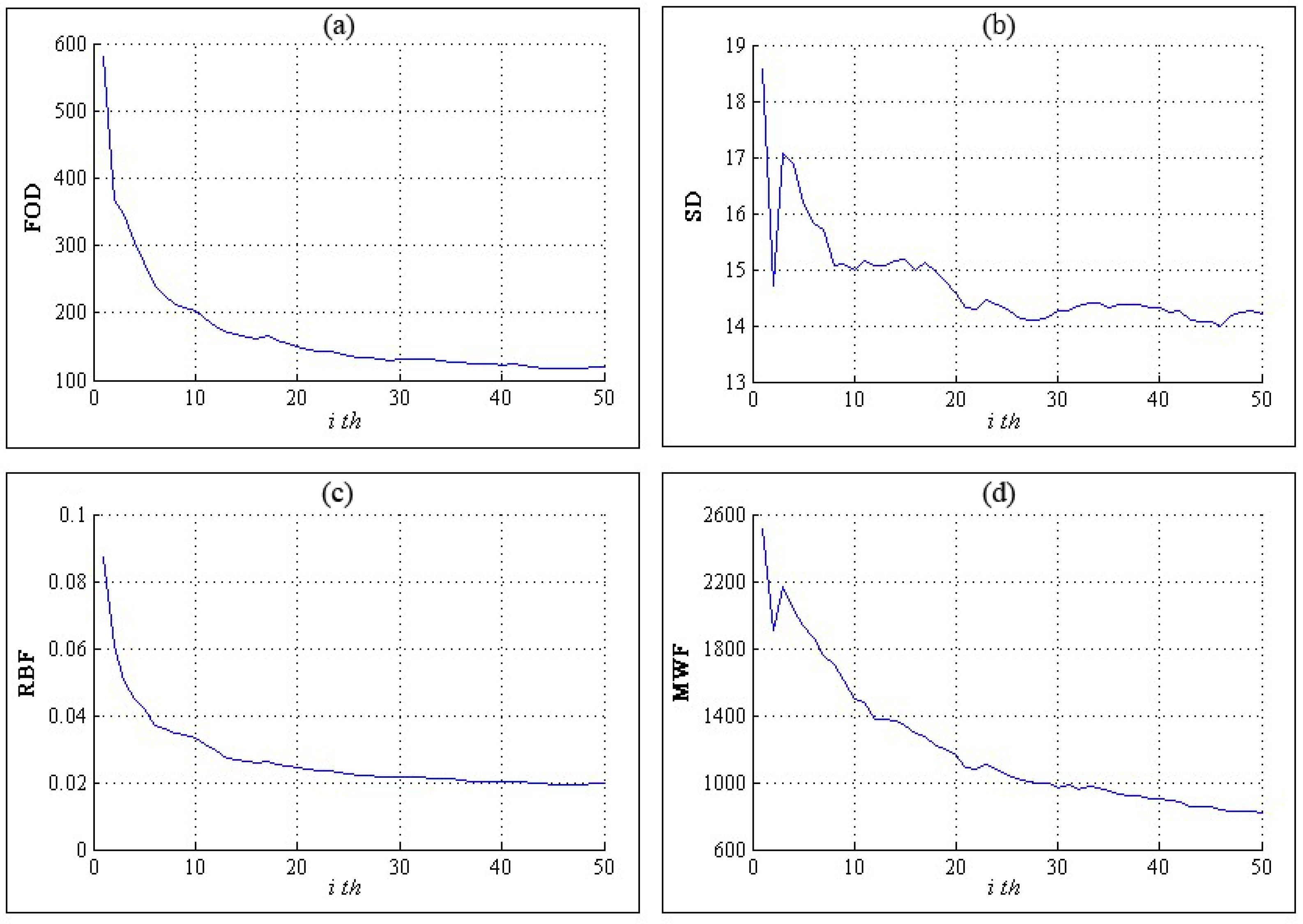
3.1. Comparison of Indices
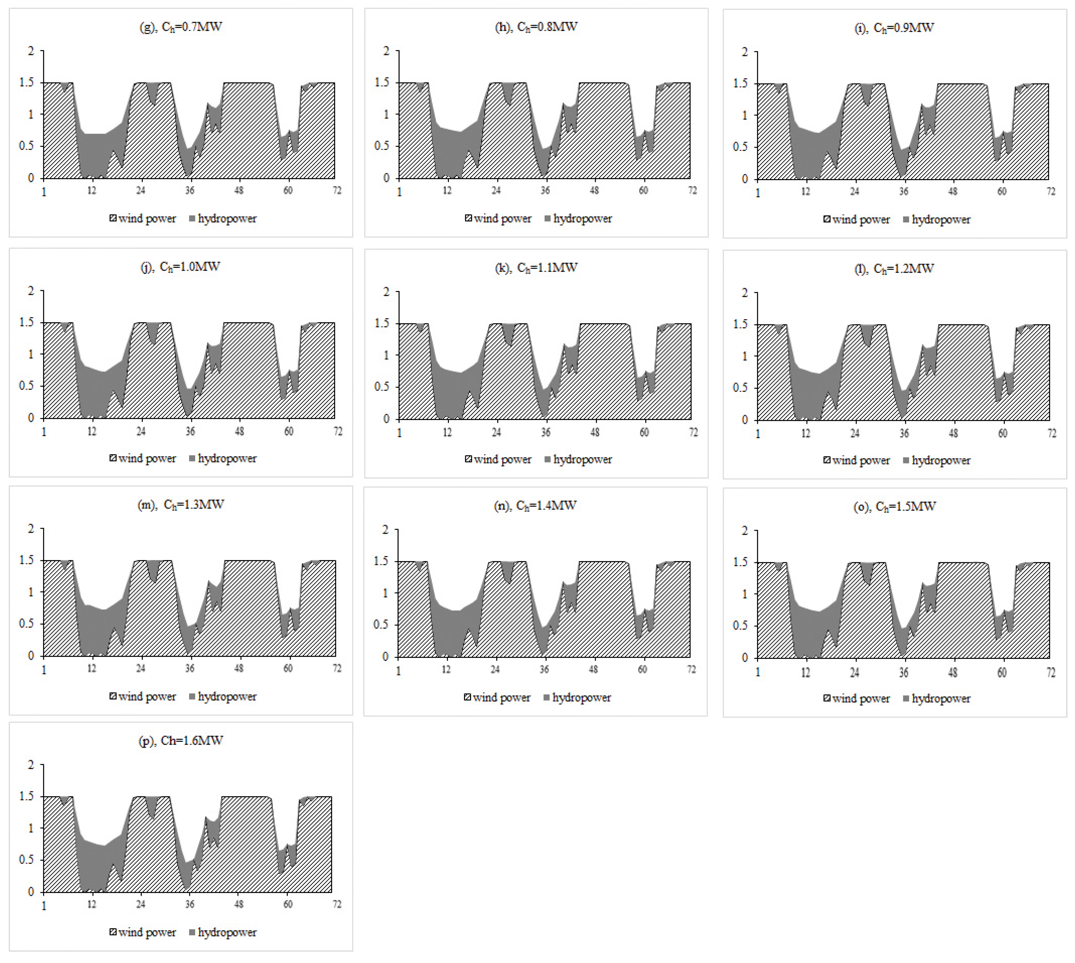
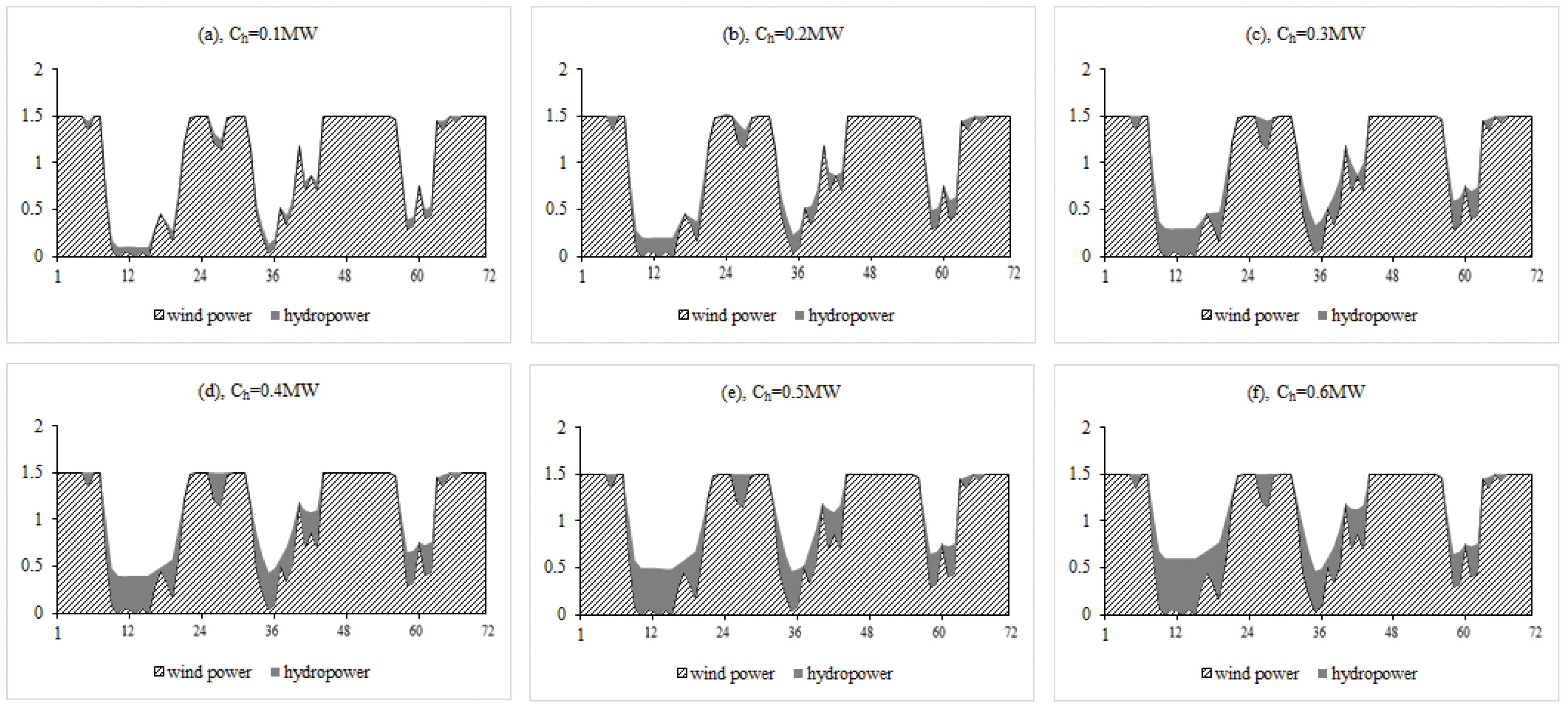
3.2. Combined Output of Wind Power and Hydropower
4. Conclusions
Acknowledgments
Author Contributions
Conflicts of Interest
References
- Ackermann, T. Wind Power in Power Systems, 2nd ed.; John Wiley: Chichester, UK, 2012. [Google Scholar]
- Sundararagavan, S.; Baker, E. Evaluating energy storage technologies for wind power integration. Sol. Energy 2012, 86, 2707–2717. [Google Scholar] [CrossRef]
- Craig, A.; Howard, R.I. Wind Power and Hydropower Integration: Concepts, Considerations and Case Studies; Nova Science Publishers Inc.: Hauppauge, NY, USA, 2012. [Google Scholar]
- Acker, T.; Robitaille, A.; Holttinen, H.; Piekutowski, M.; Tande, J. Integration of wind and hydropower systems: Results of IEA wind task 24. Wind Eng. 2012, 36, 1–18. [Google Scholar] [CrossRef]
- Bevelhimer, M.S.; McManamay, R.A.; O’Connor, B. Characterizing sub-daily flow regimes: Implications of hydrologic resolution on ecohydrology studies. River Res. Appl. 2014, 31, 867–879. [Google Scholar] [CrossRef]
- Wells, M.T. Environmental statistics with S-Plus. J. Am. Stat. Assoc. 2001, 43, 1137–1148. [Google Scholar] [CrossRef]
- Anderson, D.R.; Sweeney, D.J.; Williams, T.A. Essentials of Statistics for Business and Economics, 6th ed.; South-Western College: Cincinnati, OH, USA, 2011. [Google Scholar]
- Cassola, F.; Burlando, M.; Antonelli, M.; Ratto, C.F. Optimization of the regional spatial distribution of wind power plants to minimize the variability of wind energy input into power supply systems. J. Appl. Meteorol. Climatol. 2008, 47, 3099–3116. [Google Scholar] [CrossRef]
- Li, J.; Qiao, Y.; Lu, Z.; Li, J. An evaluation index system for wind power statistical characteristics in multiple spatial and temporal scales and its application. Proc. CSEE 2013, 33, 53–61. [Google Scholar]
- Yang, X.; Wang, W.; Xue, B.; Huang, Q. On short-term united optimal operation of wind power, thermal power and waterpower. J. Hydroelectr. Eng. 2013, 32, 199–203. [Google Scholar]
- Wang, K.; Luo, X.; Wu, L.; Liu, X. Optimal dispatch of wind-hydro-thermal power system with priority given to clean energy. Proc. CSEE 2013, 13, 27–35. [Google Scholar]
- Hoff, T.E.; Perez, R. Quantifying PV power output variability. Sol. Energy 2010, 84, 1782–1793. [Google Scholar] [CrossRef]
- Holttinen, H. Hourly wind power variations in the Nordic countries. Wind Energy 2005, 8, 173–195. [Google Scholar] [CrossRef]
- Holttinen, H. Impact of hourly wind power variations on the system operation in the Nordic countries. Wind Energy 2005, 8, 197–218. [Google Scholar] [CrossRef]
- Richter, B.D.; Baumgartner, J.V.; Wigington, R.; Braun, D.P. How much water does a river need? Freshw. Biol. 1997, 37, 231–249. [Google Scholar] [CrossRef]
- Wang, X.L.; Li, Z.W. Multi-objective optimization of combined operation of power station with wind power and pumped water power storage. J. Lanzhou Univ. Technol. 2011, 37, 78–82. [Google Scholar]
- Marcos, J.; de la Parra, Í.; García, M.; Marroyo, L.; Marroyo, L. Control strategies to smooth short-term power fluctuations in large photovoltaic plants using battery storage systems. Energies 2014, 7, 6593–6619. [Google Scholar] [CrossRef]
- McKinney, T.; Speas, D.W.; Rogers, R.S.; Persons, W.R. Rainbow trout in a regulated river below Glen Canyon Dam, Arizona, following increased minimum flows and reduced discharge variability. N. Am. J. Fish. Manag. 2001, 21, 216–222. [Google Scholar] [CrossRef]
- Haas, N.A.; O’Connor, B.L.; Hayse, J.W.; Bevelhimer, M.S.; Endreny, T.A. Analysis of daily peaking and run-of-river operations with flow variability metrics, considering subdaily to seasonal time scales. J. Am. Water Resour. Assoc. 2014, 50, 1622–1640. [Google Scholar] [CrossRef]
- Paatero, J.V.; Lund, P.D. Effect of energy storage on variations in wind power. Wind Energy 2005, 8, 421–441. [Google Scholar] [CrossRef]
- Haas, J.; Olivares, M.A.; Palma-Behnke, R. Grid-wide subdaily hydrologic alteration under massive wind power penetration in Chile. J. Environ. Manag. 2015, 154, 183–189. [Google Scholar] [CrossRef] [PubMed]
- Zimmerman, J.K.; Letcher, B.H.; Nislow, K.H.; Lutz, K.A.; Magilligan, F.J. Determining the effects of dams on subdaily variation in river flows at a whole-basin scale. River Res. Appl. 2010, 26, 1246–1260. [Google Scholar] [CrossRef]
- Violin, C.R.; Cada, P.; Sudduth, E.B.; Hassett, B.A.; Penrose, D.L.; Bernhardt, E.S. Effects of urbanization and urban stream restoration on the physical and biological structure of stream ecosystems. Ecol. Appl. 2011, 21, 1932–1949. [Google Scholar] [CrossRef] [PubMed]
- Kern, J.D.; Patino-Echeverri, D.; Characklis, G.W. The impacts of wind power integration on sub-daily variation in river flows downstream of hydroelectric dams. Environ. Sci. Technol. 2014, 48, 9844–9851. [Google Scholar] [CrossRef] [PubMed]
- Richter, B.D.; Baumgartner, J.V.; Powell, J.; Braun, D.P. A method for assessing hydrologic alteration within ecosystems. Conserv. Biol. 1996, 10, 1163–1174. [Google Scholar] [CrossRef]
- Gustafson, D.I.; Carr, K.H.; Green, T.R.; Christophe, G.; Jones, R.L.; Peter, R. Fractal-based scaling and scale-invariant dispersion of peak concentrations of crop protection chemicals in rivers. Environ. Sci. Technol. 2004, 38, 2995–3003. [Google Scholar] [CrossRef] [PubMed]
- Baker, D.B.; Richards, R.P.; Loftus, T.T.; Kramer, J.W. A new flashiness index: characteristics and applications to Midwestern rivers and streams. J. Am. Water Resour. Assoc. 2004, 40, 503–522. [Google Scholar] [CrossRef]
- Zhang, Z.; Zhou, Q.; Kusiak, A. Optimization of wind power and its variability with a computational intelligence approach. IEEE Trans. Sustain. Energy 2014, 5, 228–236. [Google Scholar] [CrossRef]
- Sauterleute, J.F.; Charmasson, J. A computational tool for the characterisation of rapid fluctuations in flow and stage in rivers caused by hydropeaking. Environ. Model. Softw. 2014, 55, 266–278. [Google Scholar] [CrossRef]
- Wang, X.X.; Mei, Y.D.; Duan, W.H.; Yang, N. Optimal Operation Models of Pumped Storage Power Station. Hydropower Autom. Dam Monit. 2008, 32, 1–3. [Google Scholar]
- Wang, X.X. Optimization of Operation of Pumped Storage Station; Wuhan University: Wuhan, China, 2008. [Google Scholar]
- Zhao, L.; Li, Y.Q. An Optimal Operation Scheduling Method of Pumped Storage Station Based on Load Curve Quantification. Mod. Electr. Power 2014, 31, 51–54. [Google Scholar]
- Wang, X.X.; Mei, Y.D. A Method and System of Stability Analysis of Power Station Operation Based on Process of Output. China Patent CN103605907A, 26 February 2014. [Google Scholar]
- Ge, H.; Guo, Q.; Sun, H.; Wang, B.; Zhang, B.; Wu, W. A load fluctuation characteristic index and its application to pilot node selection. Energies 2014, 7, 115–129. [Google Scholar] [CrossRef]
- The Nature Conservancy. Indicators of Hydrologic Alteration; Version 7, User’s manual; The Nature Conservancy: Arlington, VA, USA, 2007. [Google Scholar]
- MERRA: Modern-era Retrospective Analysis for Research and Applications. Available online: https://gmao.gsfc.nasa.gov/research/merra/ (accessed on 17 February 2016).


| Index | Description | Source/Reference |
|---|---|---|
| First Order Difference | Reference [8] | |
| SD | Carl Friedrich Gauss | |
| Richards-Baker Flashiness (RBF) | Reference [27] | |
| Mei-Wang Fluctuation (MWF) | This study |
| Disposal | FOD | SD | RBF | MWF |
|---|---|---|---|---|
| moving average | ★ | ★ | ★ | ★ |
| repeating | ★ | △ | △ | ★ |
| zoom | △ | △ | △ | ★ |
| overlay of wind speed | ★ | ★ | ★ | ★ |
| overlay of runoff | △ | ★ | △ | ★ |
| wind speed (m/s) | 3 | 4 | 5 | 6 | 7 |
| wind power (MW) | 0.03 | 0.09 | 0.18 | 0.32 | 0.52 |
| wind speed (m/s) | 8 | 9 | 10 | 11 | 22 |
| wind power (MW) | 0.78 | 1.09 | 1.42 | 1.5 | 1.5 |
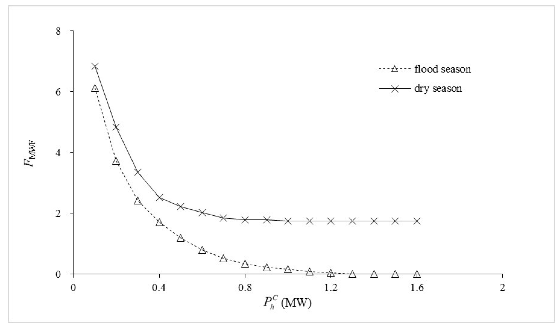
| Hydropower Capacity (MW) | 0.1 | 0.2 | 0.3 | 0.4 | 0.5 | 0.6 | 0.7 | 0.8 | |
| Minimum | Flood Season | 6.13 | 3.74 | 2.41 | 1.71 | 1.20 | 0.8 | 0.52 | 0.34 |
| Dry Season | 6.84 | 4.84 | 3.35 | 2.53 | 2.22 | 2.02 | 1.85 | 1.78 | |
| Hydropower Capacity (MW) | 0.9 | 1 | 1.1 | 1.2 | 1.3 | 1.4 | 1.5 | 1.6 | |
| Minimum | Flood season | 0.22 | 0.15 | 0.07 | 0.04 | 0 | 0 | 0 | 0 |
| Dry season | 1.78 | 1.74 | 1.74 | 1.74 | 1.74 | 1.74 | 1.74 | 1.74 | |
© 2016 by the authors; licensee MDPI, Basel, Switzerland. This article is an open access article distributed under the terms and conditions of the Creative Commons by Attribution (CC-BY) license (http://creativecommons.org/licenses/by/4.0/).
Share and Cite
Wang, X.; Mei, Y.; Cai, H.; Cong, X. A New Fluctuation Index: Characteristics and Application to Hydro-Wind Systems. Energies 2016, 9, 114. https://doi.org/10.3390/en9020114
Wang X, Mei Y, Cai H, Cong X. A New Fluctuation Index: Characteristics and Application to Hydro-Wind Systems. Energies. 2016; 9(2):114. https://doi.org/10.3390/en9020114
Chicago/Turabian StyleWang, Xianxun, Yadong Mei, Hao Cai, and Xiangyu Cong. 2016. "A New Fluctuation Index: Characteristics and Application to Hydro-Wind Systems" Energies 9, no. 2: 114. https://doi.org/10.3390/en9020114