Analyzing Crude Oil Spot Price Dynamics versus Long Term Future Prices: A Wavelet Analysis Approach

Abstract

The West Texas Intermediate (WTI) spot price shows high volatility and in 2014 and 2015 when quoted prices declined sharply, long-term prices in future markets were less volatile. These prices are different and diverge depending on how they process fundamental and transitory factors. US tight oil production has been a major innovation with significant macroeconomic effects. In this paper we use WTI spot prices and long-term futures prices, the latter calculated as the expected value with a stochastic model calibrated with the futures quotes of each sample day. These long-term prices are the long-term equilibrium value under risk neutral measurement. In order to analyze potential time-scale relationships between spots and future, we perform a wavelet cross-correlation analysis using a novel wavelet graphical tool recently proposed. To check the direction of the causality, we apply non-linear causality tests to raw data and log returns as well as to the wavelet transform of the spot and futures prices. Our results show that in the spot and futures markets for the period 24 February 2006–2 April 2016 there is a bi-directional causality effect for most time scales (from intra-week to biannual). This suggests that spot and futures prices react simultaneously to new information.

1. Introduction

The West Texas Intermediate (WTI) spot price, one of the world’s most important crude oil markets (Deng and Sakurai [1]), usually shows high volatility and in 2015 its prices declined sharply. At the same time, long-term WTI futures prices were less volatile: They also underwent significant price declines, but to a lesser extent. These prices are different and diverge depending on how they process fundamental and transitory factors. For instance, a relevant recent innovation with significant macroeconomic effects is US tight oil production. This term refers to all low-permeability crude oil production formations, including shale formations.

Changes in spot and futures prices may be due to fundamental shifts in supply and demand; but they could also be due to speculation. Knittel and Pindyck [2] show that futures contracts are the easiest instrument of speculation to use for the lowest cost; moreover a substantial fraction of futures contracts are held by producers and industrial consumers to hedge risk, e.g., in the case of refineries. Knittel and Pindyck [2] conclude that the behavior of inventories and the futures-spot spread is simply inconsistent with the view that speculation has been a significant driver of spot prices. A shift in oil market fundamentals can affect supply and demand and the effect may be short-term or long-term. Extreme cold weather events and an unexpected shutdown of some base power plants are examples of short-term shifts in fundamentals of demand and supply, respectively. Other shifts have more permanent effects, such as increase in crude oil demand in China and other developing countries, along with the development of tight oil extraction technology result in a supply shift.

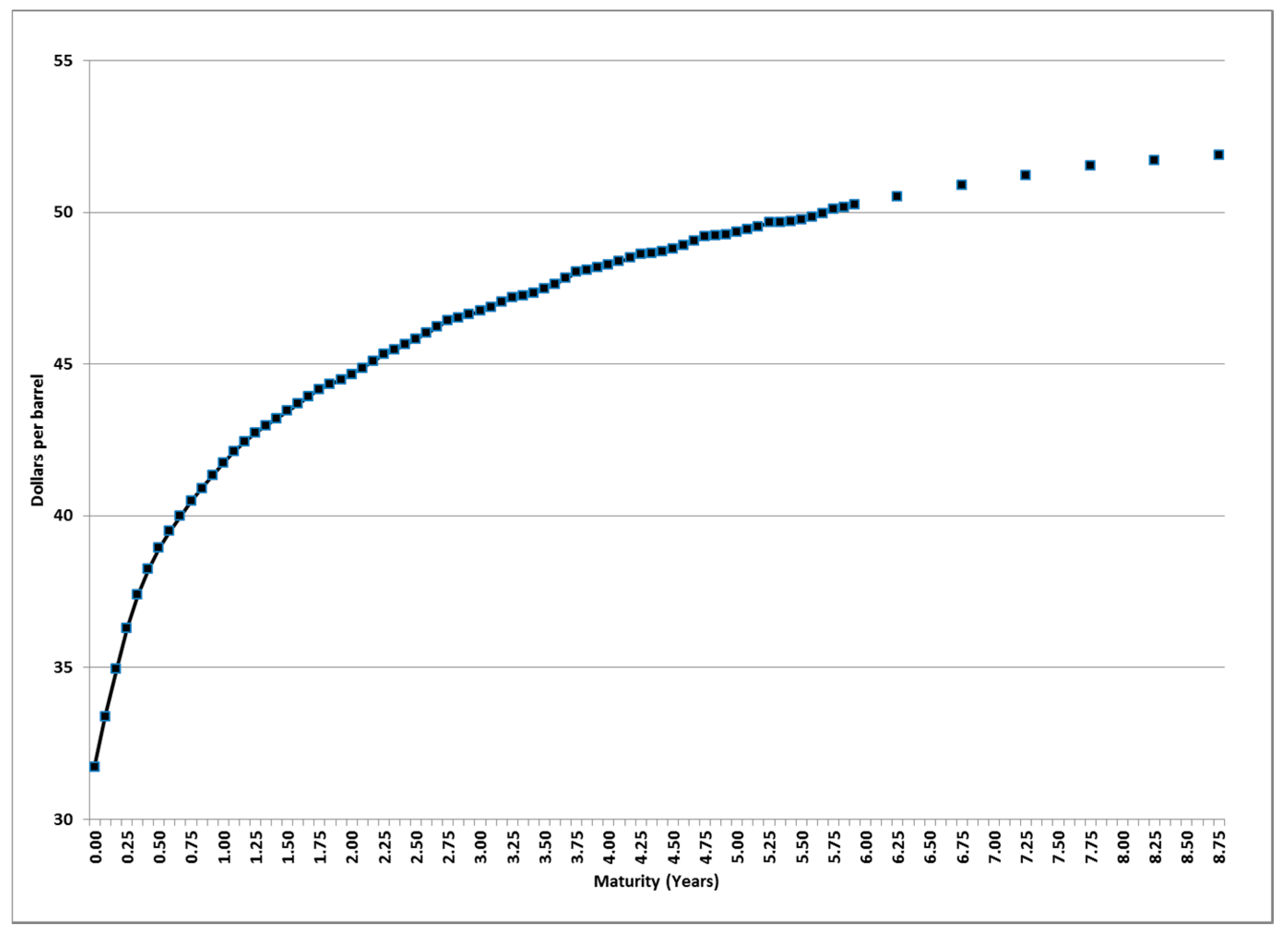
Figure 1 shows the term structure of WTI Futures Prices for the 2 April 2016, which is the last day of the sample. The shape of the futures curves is very important for pricing crude oil barrels for the following reason: this shape enables us to observe the spread between futures and spot prices, which is equivalent to the storage price. The situation at the end of 2015 and early 2016 is such that spot prices are lower than long maturity futures prices (contango). The shape of Figure 1 suggests a mean reverting stochastic model for the crude oil price, because the price on the futures market tends towards an equilibrium long-term price as maturity periods increase. This behavior is common on almost all days when futures prices are above spot prices. A similar behavior occurs on almost all days when spot prices are above the prices of futures markets. In these cases a long-term price equilibrium can also be found. However, in the sample there are a few days in which no long-term equilibrium prices can be found using the daily futures term structure because the temporary structure of these days shows an accelerated rise or decline. In these few cases, the price of the future with the longest maturity on that day provides information for an alternative estimate using the last spread between the last future and the long-term equilibrium price.

It is clearly established that, both spot and futures prices are relevant for the economy, but not less important is the interrelationship between spot and futures prices. For instance, the lead-lag relationship between crude oil spot and futures markets is a debatable issue, as can be corroborated in the many publications on this topic since the seminal 1999 paper by Silvapulle and Moosa [3].

Most studies of the relationship between spot and long-term future prices on the crude oil market are based mainly on the estimation of Pearson’s and Spearman’s correlation coefficients, the cross-correlation function, cointegration theory (bi- and multivariate) or the use of generalized VAR or (G)ARCH models [3,4,5,6,7]. However, cointegration theory can only tackle short-run vs. long-run time horizons and the VAR and (G)ARCH approaches are sensitive to model specifications [8]. By contrast, from a practical point of view, oil time series can be not stationary and involve heterogeneous agents who make decisions over different time horizons and operate on different time scales (frequencies) [9,10,11,12]. A mathematical tool that can handle non-stationaries time series, study interrelationships between time series and it is able to work in the combined time-and-scale domain, it is the wavelet cross-correlation via the Maximal Overlap Discrete Wavelet Transform (MODWT) [13,14]. Furthermore, the MODWT obtain an overview of the temporal changes in spectral dynamics of a time series under study. For all these reasons, this statistical tool is adequate to analyze the long-term futures and spot prices. Furthermore, to date the wavelet cross-correlation (via MODWT) has not been widely used to study the correlation and co-movements between spot and long-term futures oil prices.

Inspired by Chang and Lee [12] and Alzahrani et al. [15], in this paper we contribute to the literature on the lead–lag relationship between spot and futures crude oil prices in the following way. We use all the futures contracts of each day and we estimate the long-term equilibrium price to which the price of the futures markets when the maturity period increases in such a way that our sample has futures price quotes with a maximum maturity of 8.92 years. To estimate the long-term equilibrium price we use a recently proposed stochastic model (Section 2.2). As a first approach, potential relationships between spot and long-term futures prices estimated with the stochastic model are studied by means of the classical cross-correlation function. Then we estimate the wavelet cross-correlation between the time series under study. We also apply non-parametric and non-linear causality tests (Diks and Panchenko [16]) to the wavelet decomposition of the spot and futures prices. Lastly, we use a useful, novel graphical tool proposed by Polanco-Martínez and Fernández-Macho [17] that helps with the interpretation of wavelet cross-correlation analysis.

The rest of the paper is organized as follows: Section 2 describes the sample data, the stochastic diffusion model, the wavelet methodology and the causality tests. The results and their discussion are presented in Section 3. Finally, Section 4 concludes the paper.

2. Material and Methods

2.1. Data Description

Our sample consists of 161,274 daily futures prices from the Intercontinental Exchange (ICE). We focus on the period from 24 February 2006 to 2 April 2016, i.e., nearly ten years.

Table 1. WTI Crude Futures Market Specifications. Source: Intercontinental Exchange (ICE).

Contract Size	1000 barrels
Units of Trading	Any multiple of 1000 barrels
Currency	US dollars and cents
Clearing	ICE Clear Europe guarantees financial performance of all ICE Futures Europe contracts registered with it by its clearing Members. All ICE Futures Europe Member companies are either members of ICE Clear Europe, or have a clearing agreement with a Member who is a member of ICE Clear Europe.
Contract Listing	Up to 108 consecutive months
Last trading day	Trading shall cease at the end of the designated settlement period on the 4th US business day prior to the 25th calendar day of the month preceding the contract month. If the 25th calendar day of the month is not a US business day the Final Trade Day shall be the Trading Day which is the fourth US business day prior to the last US business day preceding the 25th calendar day of the month preceding the contract month.
Settlement	The West Texas Intermediate Light Sweet Crude Oil futures contract is cash settled against the prevailing market price for US light sweet crude. It is a price in USD per barrel equal to the penultimate settlement price for WTI crude futures as made public by NYMEX for the month of production per 2005 ISDA Commodity Definitions.

shows some market specifications. Crude oil futures prices are determined by the expectations of producers, consumers and speculators for a future date.

Table 2. Some Futures Contract volatility levels according to their maturity.

Maturity	Number of Observations	Volatility of Returns
~1 month	2571	0.3175
6 Months	2571	0.2859
12 Months	2571	0.2602
18 Months	2571	0.2452
24 Months	2571	0.2324
30 Months	2548	0.2250
36 Months	2420	0.2201
42 Months	2246	0.2176
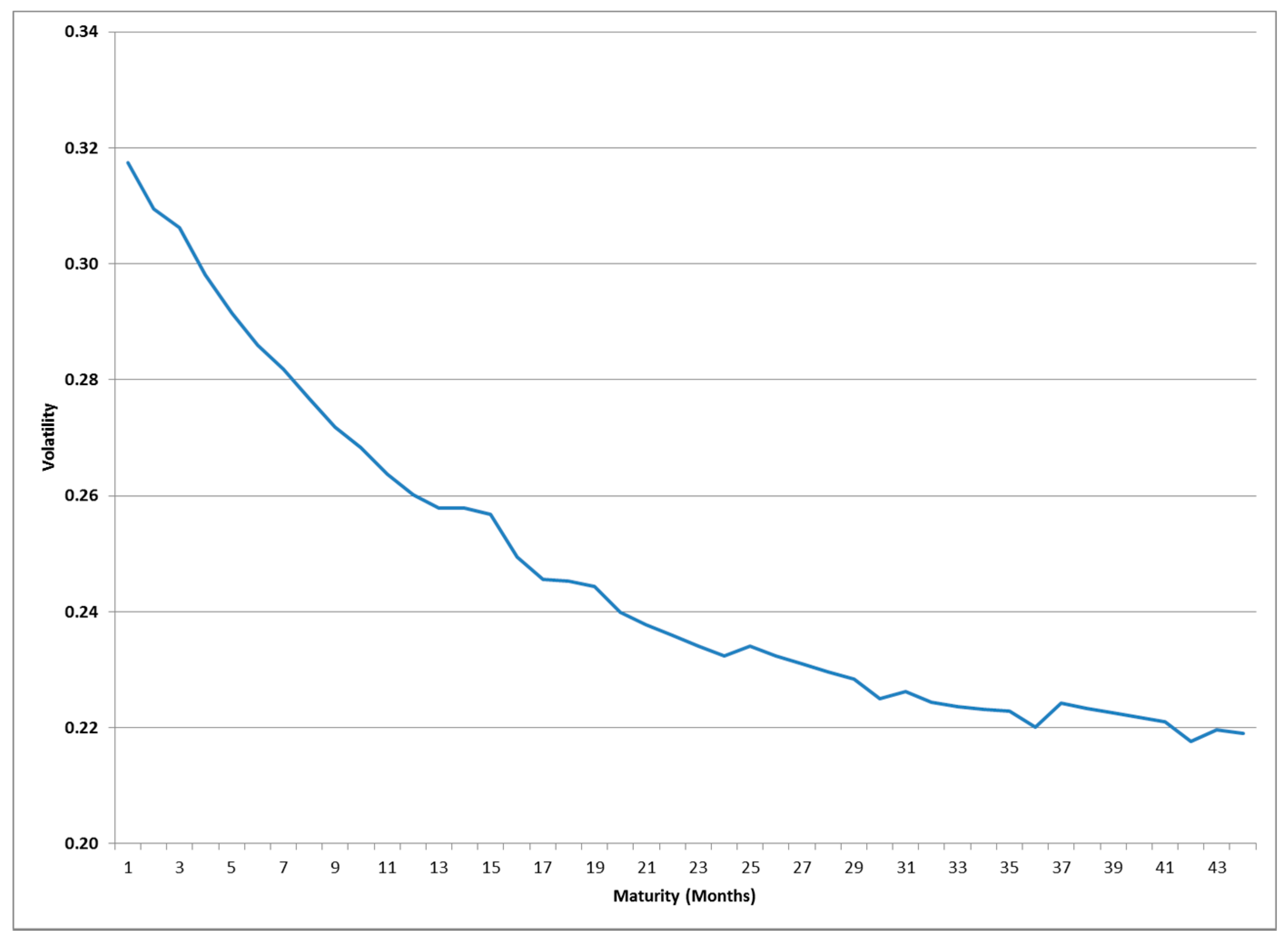
48 Months	2189	0.2155

shows the number of observations and the volatility of returns of some futures contracts from the data sample classified according to their maturity. As can be seen, the volatility decreases as maturity increases: This is known as the Samuelson effect. That is, energy futures contracts usually show decreasing volatility as a function of the remaining lifetime of the contract T-t, as T-t decreases, volatility increases and the spot price converges with the futures contract price so that F(T, T) = S_T. This effect/behavior can be observed more easily in Figure 2. Crude oil futures prices are determined by the expectations of producers, consumers and speculators for a future date.

2.2. The Stochastic Model

The crude oil spot price denoted by S can be assumed to evolve stochastically in accordance with a mean-reverting process (MR) as per Equation (1):

$$d{S}_t=k(S_m-S_t)dt+\sigma S_{t}dW$$

(1)

In this equation $S_m$ is the long-term equilibrium value towards which the spot price $S_t$ tends to revert in the long-term, k is the speed of reversion that determines how the expected value of $S_t$ approximates in time to the long-term equilibrium value $S_m$, σ is the volatility and $dW=\epsilon (t)\sqrt{dt}$ is the increment of a Wiener process with $\epsilon (t):N(0,1)$. Let λ be the market price of risk, then the behavior in the risk-neutral word (this is the futures market case) is:

$$d{S}_t=\left[k(S_m-S_t)-\lambda S_t\right]dt+\sigma S_{t}dW$$

(2)

Abadie and Chamorro (2013) [18] show that in the risk-neutral world the expected value under the equivalent martingale measure or risk-neutral measure in the moment t for the future price with maturity T is:

$$F(t,T)=\frac{k{S}_m}{k+\lambda }+[S_t-\frac{k{S}_m}{k+\lambda }]e^{-(k+\lambda )(T-t)}$$

(3)

A similar Equation (4) can be used with the future with the nearest maturity denoted by T₁ to estimate the future price with maturity T₂:

$$F(t,T_2)=\frac{k{S}_m}{k+\lambda }+[F(t,T_1)-\frac{k{S}_m}{k+\lambda }]e^{-(k+\lambda )(T_2-T_1)}$$

(4)

Equation (4) enables estimates for each day to be drawn up for the values $k+\lambda$ and $\frac{k{S}_m}{k+\lambda }$.

In the long-term there is a long-term equilibrium value given by Equation (5):

$$F(t,\infty )=\frac{k{S}_m}{k+\lambda }=S^{*}$$

(5)

Initially we calculate k + λ and S* for each day using nonlinear least squares, which results in 2571 values of each parameter. More information about the parameters calculation can be found in Appendix A. We obtain the time-series $S_t^{*}$, but there are some outliers, so we refine it using the procedure described in Appendix B.

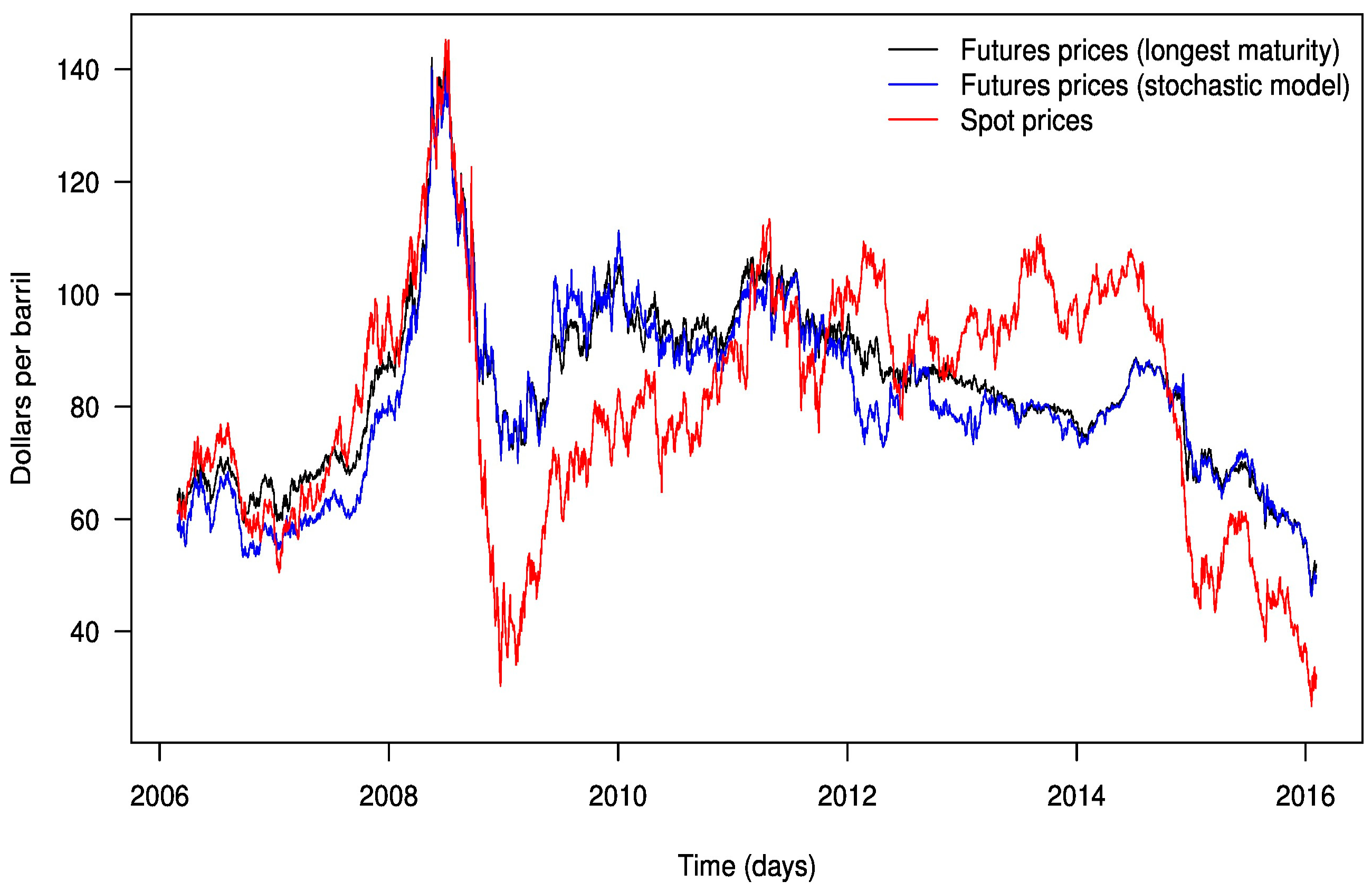
Figure 3 shows the lower volatility of futures contracts with long maturity periods on every day. Since 2008 these futures prices have been higher than spot prices when the latter have fallen considerably, and below them when spot prices have been very high. Figure 3 also shows a peak of $145 and a rise in oil prices in July 2008. According to Kaufmann and Ullman [4], this rise was caused by changes in market fundamentals and speculation. These authors conclude that the increase anticipated by prices set in futures markets, exacerbated by speculators, was transmitted to the spot market. On the other hand, in 2015 futures prices were above the spot price, reflecting a situation of contango in the market.

Table 3. Descriptive statistics for spot and long-term futures prices.

Statistics	Spot		Futures (Stochastic Model)		Futures (Longest Maturities)
	Raw Data	Log Returns	Raw Data	Log Returns	Raw Data	Log Returns
Mean	80.663	−3 × 10−4	83.592	−1 × 10−4	81.252	−1 × 10−4
Median	82.800	2 × 10−4	84.300	1 × 10−4	80.145	2 × 10−4
Max.	145.310	0.164	142.770	0.067	140.283	0.066
Min.	26.680	−0.128	47.150	−0.071	46.276	−0.074
Std. Dev.	21.626	0.024	15.081	0.013	15.993	0.014
Skewness	−0.128	0.129	0.625	−0.199	0.501	−0.095
Kurtosis	−0.375	5.025	1.231	3.319	0.612	1.842
Jarque-Bera	21.954	2717.811	330.759	1199.947	148.398	368.677
p-value	0.000	0.000	0.000	0.000	0.000	0.000
Dickey-Fuller	−1.553	−12.721	−1.801	−14.186	−1.888	−13.943
p-value	0.767	0.010	0.663	0.010	0.626	0.010

reports the descriptive statistics for spot and futures prices obtained as the longest maturities and estimated by a stochastic model, Jarque-Bera test for normality (Jarque and Bera [19]) as implemented in the R package tseries (Trapletti and Hornik [20]) as well as the Augmented Dickey-Fuller (ADF) unit-root test (Dickey and Fuller [21]) as implemented in the R package tseries (Trapletti and Hornik [20]) with structural breaks. A first glance, the skewness shows that in all cases the data sets have a slight asymmetric probability distribution. On the other hand, the kurtosis values show that none of them have a value close to 3 (the theoretical value for a Gaussian probability distribution), except the log returns for the futures prices estimated by a stochastic model. However, the Jarque-Bera test indicates that none of the probability distributions of these time series appear to be normally distributed. Table 3 also reports the results of ADF unit-root test for the levels of the series as well as the log returns. When the ADF test is applied to the raw data, we fail to reject to reject the null hypothesis for all the time series. Nevertheless, when the test is applied to the log returns, all nulls are rejected consistently. Thus, the test reveals that all the raw data sets are integrated of order one, that is, are non-stationaries whereas the log returns do not contain a unit-root indicating that these series are stationaries.

2.3. The Wavelet Methodology

Discrete Wavelet Transform (DWT) [13,14] is a mathematical tool that can handle non-stationary time series and which works in the combined time-and-scale domain. There are various algorithms for computing the DWT. In this paper we use the Maximal Overlap Discrete Wavelet Transform (MODWT) because of its advantages over the classical DWT. To begin with, the MODWT can tackle any sample size N, while the DWT of level J restricts the sample size to a multiple of 2J. Also, more importantly, the MODWT is invariant to circular shifting of the time series under study, while the DWT is not. Furthermore, both the DWT and MODWT can be used to analyze variance based on wavelet and scaling coefficients, but the MODWT wavelet variance estimator of the wavelet coefficients is asymptotically more efficient than the equivalent estimator based on DWT [13,14,22]. The MODWT is used to compute wavelet variances, wavelet correlations (WC) and cross-correlations (WCC) of bivariate time series [13,14]. Several applications of the DWT and MODWT can be found in economic and financial literature (see e.g., [8,13,23,24]) and to a lesser extent in energy studies [25,26,27]. Nevertheless, to date the WCC (via MODWT) has not been widely used to study the correlation and co-movements between spot and long-term futures oil prices (though some exceptions are discussed below).

Yousefi et al. [9] propose the wavelet analysis approach as a possible vehicle for investigating market efficiency in futures markets for oil (prediction of oil prices). More recently, Naccache [10], Aguiar-Conraria and Soares [28], Benhmad (2012) [25] and Reboredo and Rivera-Castro [11], among others, address the question of the link between oil prices and the macroeconomy using world data and a time scale decomposition based on the theory of wavelets. However, the first study of the relationship between spot and futures prices of crude oil using wavelet analysis was not performed until 2015 by Chang and Lee [12]. They investigate the time-varying correlation and the causal relationship between crude oil spot and futures prices using wavelet coherency analysis. Chang and Lee) [12] find significant dynamic correlations between these variables in the time–frequency domain, in a such way that spot and futures prices contribute to the dynamics of the long-run equilibrium. They recommend that future studies focusing on the behavior of oil prices should consider the characteristics of the time–frequency space and lead–lag dynamic relationships. However, Chang and Lee [12] use futures contracts with one, two, three, and four months, i.e., futures contracts with a very short-term maturity (around 0.33 years). They do not take into account the causal relationship between oil spot and futures prices. This task was tackled more recently by Alzahrani et al. [15] in the first combined study that mixes wavelet analysis and non-linear causality. Alzahrani et al. [15] find consistent bidirectional causality between spot and futures oil markets on different time scales.

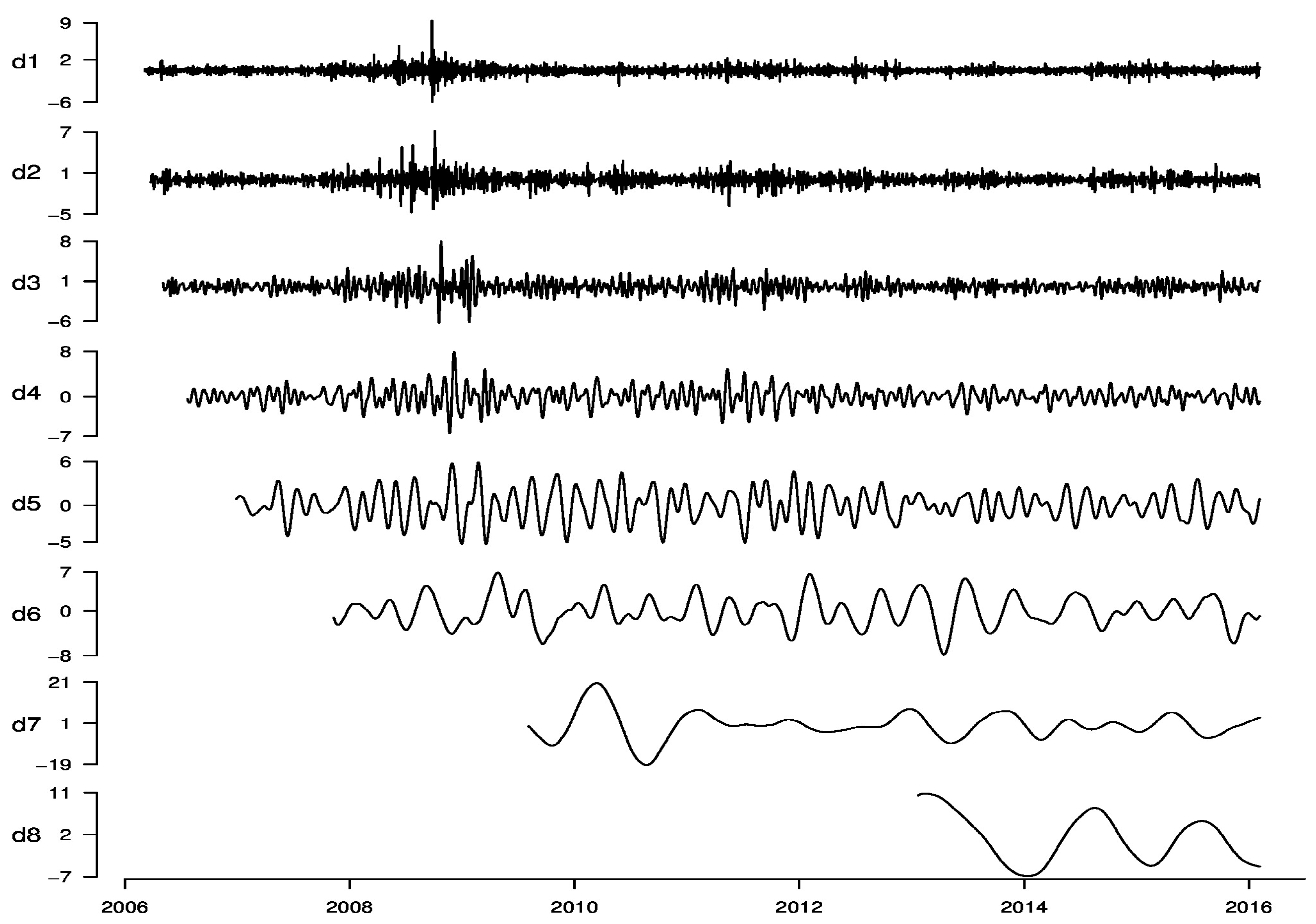
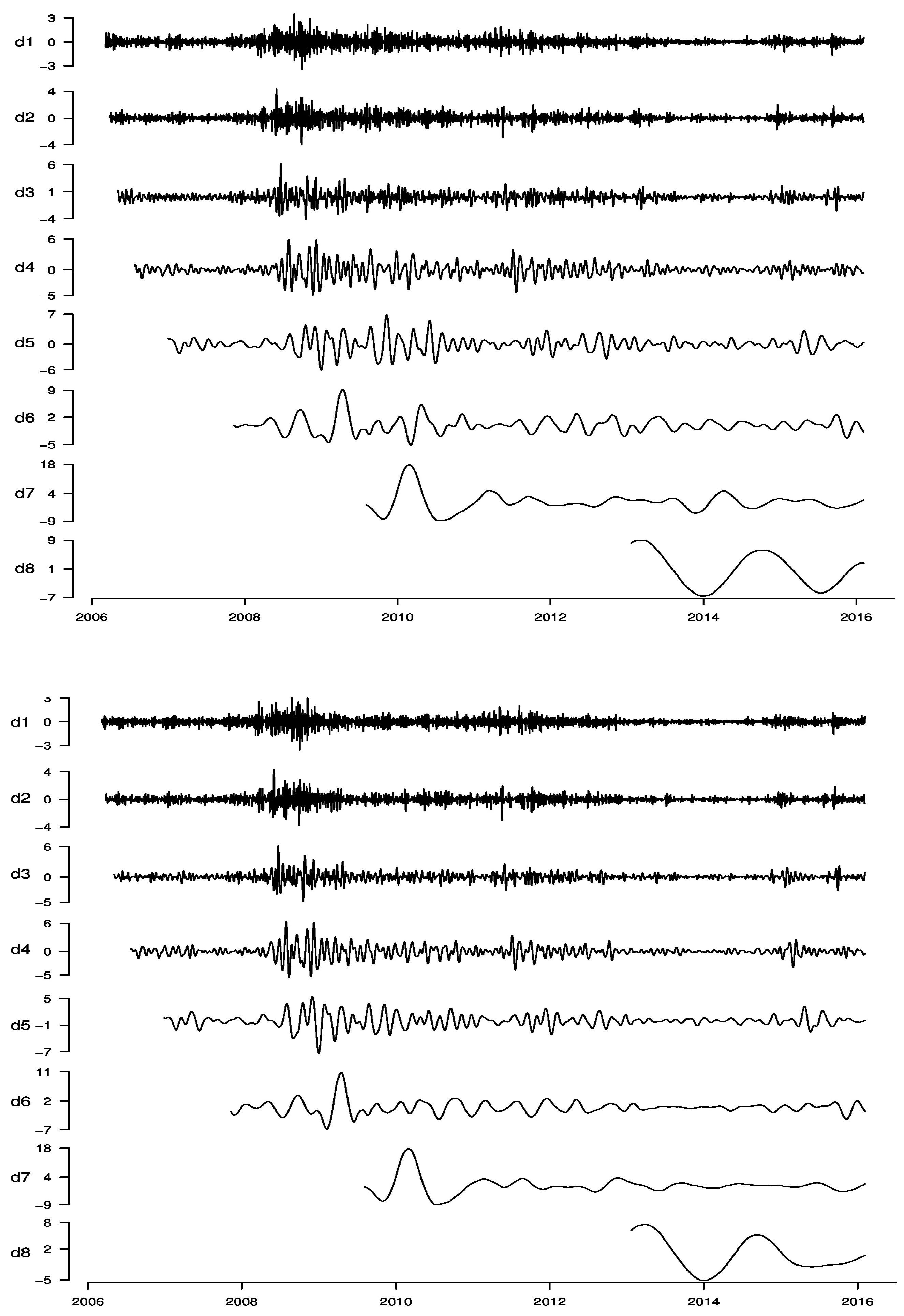
In order to decompose the daily oil time series (Figure C1; Appendix C) in this work, we have applied the MODWT with a Daubechies least asymmetric (LA) wavelet filter of length L = 8, commonly denoted as LA(8) [13,29]. The maximum decomposition level J is given by $lo{g}_2\left(N\right)$ [13,14], which in this case is J = 8, so the MODWT produces eight wavelet coefficients and one scaling coefficient, that is,${\tilde{w}}_{1,t},\dots ,{\tilde{w}}_{8,t}$ and ${\tilde{v}}_{8,t}$, respectively.

Note that the level of the transform defines the scale of the respective wavelet coefficients ${\tilde{w}}_{t,j}$. In particular, for all families of Daubechies compactly supported wavelets the level j wavelet coefficients are associated with changes at an effective scale of ${\lambda }_j=2^{j-1}$ days (in our case) [23]. Moreover, the MODWT utilizes approximate ideal bandpass filters with bandpass given by the frequency interval $\left[1/2^{j+1},1/2^j\right)$ for scale levels 1 ≤ j ≤ J. Inverting the frequency range and multiplying by the appropriate time units ∆t (one day in our case) gives the equivalent periods of $\left(2^j,2^{j+1}\right]\Delta t$ days for scale levels 1 ≤ j ≤ J [29]. This means that in our case study, with daily data, the scales ${\lambda }_j$, j = 1, 2, …, 8 (associated with changes of 1, 2, 4, 8, 16, 32, 64 and 128 days) of the wavelet coefficients are associated with day periods of, respectively, 2–4 (includes most intraweek scales), 4–8 (including the weekly scale), 8–16 (fortnightly scale), 16–32 (monthly scale), 32–64 (monthly to quarterly scale), 64–128 (quarterly to biannual scale), 128–256 (biannual scale), and 256–512 days (annual scale).

In order to analyze the relationship between spot and long-term futures prices from the crude oil market time series at different time/period horizons, we compute the wavelet cross-correlation (WCC). We follow the methodology for computing the wavelet transform (MODWT) and WCC given by Gencay et al. [13], as implemented in the R package Waveslim [30]. To obtain a graphical interpretation of wavelet correlation and cross-correlation analysis, we use the R package W2CWM2C [17,31].

The MODWT unbiased estimator of the wavelet correlation for scale ${\lambda }_j$ between two time series X and Y can be expressed as follows [13]:

$${\tilde{\rho }}_{XY}=\frac{cov({\tilde{W}}_{X,j,t},{\tilde{W}}_{Y,j,t})}{\sqrt{var\{{\tilde{W}}_{X,j,t}\}var\{{\tilde{W}}_{Y,j,t}\}}}=\frac{{\tilde{\gamma }}_{XY}\left({\lambda }_j\right)}{{\tilde{\sigma }}_X\left({\lambda }_j\right){\tilde{\sigma }}_Y\left({\lambda }_j\right)}$$

(6)

where ${\tilde{\gamma }}_{XY}\left({\lambda }_j\right)$is the unbiased estimator of the wavelet covariance between wavelet coefficients ${\tilde{W}}_{X,j,t}$ and ${\tilde{W}}_{Y,j,t}$, and ${\tilde{\sigma }}_X\left({\lambda }_j\right)$ and ${\tilde{\sigma }}_Y\left({\lambda }_j\right)$ are the unbiased estimators of the wavelet variances for X and Y respectively, associated with scale ${\lambda }_j$. An unbiased estimator of the wavelet variance based on the MODWT is defined [13] by:

$${\tilde{\sigma }}_X^2\left({\lambda }_j\right)=\frac{1}{{\tilde{N}}_j}{\displaystyle \sum }_{t=L_j-1}^{N-1}{\tilde{W}}_{j,t}^2$$

(7)

where $\{{\tilde{W}}_{\mathrm{j},\mathrm{t}}\}$ is the jth level MODWT wavelet coefficients for the time series X,$L_j=(2^j-1)(L-1)+1$ is the length of scale ${\lambda }_j$ wavelet filter, and $N_j=N-L_j+1$ is the number of the coefficients not affected by the boundary.

The MODWT unbiased estimator of the wavelet cross-correlation for scale ${\lambda }_j$ and lag τ between two times series X and Y is defined by [13]:

$${\tilde{\rho }}_{XY,\tau }\left({\lambda }_j\right)=\frac{cov({\tilde{W}}_{X,j,t},{\tilde{W}}_{Y,j,t+\tau })}{\sqrt{var\{{\tilde{W}}_{X,j,t}\}var\{{\tilde{W}}_{Y,j,t+\tau }\}}}=\frac{{\tilde{\gamma }}_{XY,\tau }\left({\lambda }_j\right)}{{\tilde{\sigma }}_X\left({\lambda }_j\right){\tilde{\sigma }}_Y\left({\lambda }_j\right)}$$

(8)

where ${\tilde{\gamma }}_{XY,\tau }$is the unbiased estimator of the wavelet cross-covariance, and${\tilde{\sigma }}_X\left({\lambda }_j\right)$ and ${\tilde{\sigma }}_Y\left({\lambda }_j\right)$ are the unbiased estimators of the wavelet variances of X and Y, respectively. Note that the WCC is roughly analogous to its Fourier counterpart, the magnitude squared coherence, but the WCC is related to bands of scales (frequencies) [32]. The WCC ${\tilde{\rho }}_{XY,\tau }\left({\lambda }_j\right)\in \left[-1,1\right]$, and is used to determine lead/lag relationships between two time series on different scales ${\lambda }_j$.

The confidence interval for the WCC is based on an extension of the classical result on the Fisher’s Z-transformation of the correlation coefficient [32]. Thus, an approximate 100(1$-$2p)% confidence interval for the WCC is given by $\tanh \{h\left[{\tilde{\rho }}_{XY}\left({\lambda }_j\right)\right]\pm {\varphi }^{-1}\left(1-p\right)/\sqrt{{\tilde{N}}_j-3}\}$, where ${\widehat{N}}_j=N_j-\left(L-2\right)\left(1-2^{-j}\right)$, ${\varphi }^{-1}\left(p\right)$ is the 100p% percentage point for the standard normal distribution, and $h\left({\tilde{\rho }}_{XY}\right)=tan{h}^{-1}\left({\tilde{\rho }}_{XY}\right)$ [13,32].

2.4. Nonlinear Causality Tests

Savit [33] argued that financial and commodity markets are dynamical systems that could manifest nonlinearities, and he also argued that these elude common linear statistical tests (including linear causality tests). Baek and Brock [34] proposed a nonparametric test for detecting nonlinear causal relationships based on the correlation integral, which is an estimator of spatial dependence across time. Later on, Hiemstra and Jones [35] provided an improved version of Baek and Brock [34]. However, despite the test of Hiemstra and Jones [35] is (probably) the most used nonlinear causality test in economics and finance (there are others nonlinear causality tests developed to analyze this kind of data, but these are not commonly used, e.g., Bell et al. [36]; Su and White [37]; among others). However, it tends to over-reject the null hypothesis if it is true (Diks and Panchenko [16,38]). For this reason, Diks and Panchenko [16] proposed a new nonparametric and nonlinear Granger causality test to avoid the over-rejection. In our work, we use the causality test of Diks and Panchenko [16], as implemented in the C program GCTtest, which is freely available on the Internet [39]. In addition, we use the test of Toda and Yamamoto [40] only to analyze potential causal relationships in raw data. This test is implemented in the R language and it is available freely on the web [41].

3. Results and Discussion

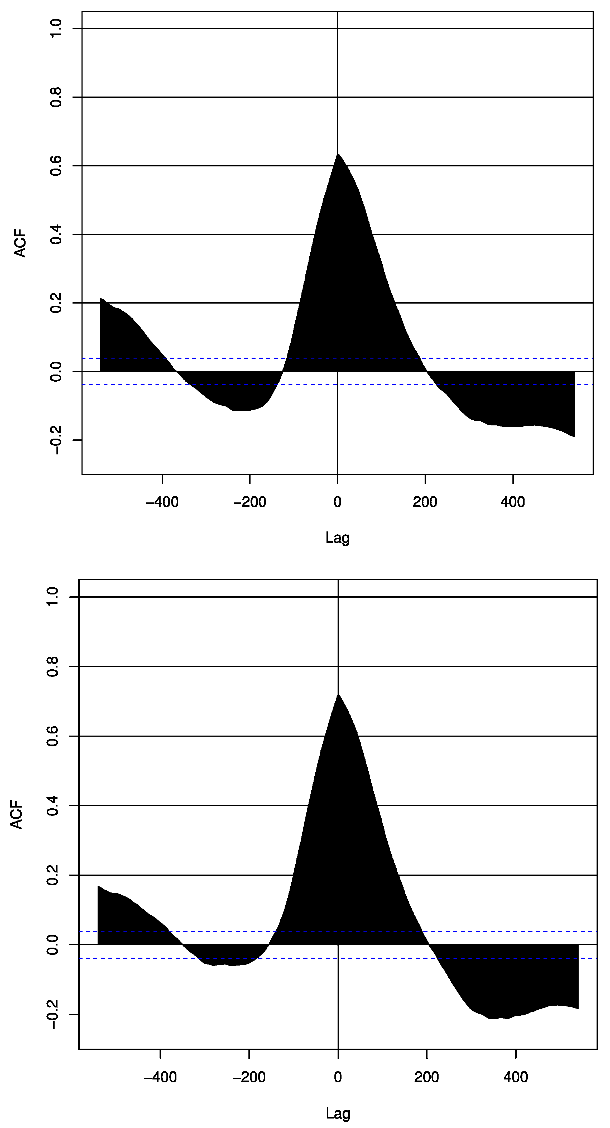
The cross-correlation analysis (Figure 4) between long-term futures prices estimated by means of a stochastic model and spot prices reveals a relatively strong positive correlation that is statistically significant around lag-0 (r = 0.62) and a right-side asymmetry (other lags are present but are disregarded due to the difficulty of interpretating them). These features are also found in the cross-correlation between “last future prices” (the price of the future with the longest maturity period on that day) and spot prices, although the correlation coefficient around lag-0 is a little larger (r = 0.71) than the one when the stochastic model is used to compute the futures. Cross-correlation is a useful statistical tool for looking for correlation between two time series. However, due to the fact that correlation does not necessarily imply causation, it is not the best tool for analyzing potential cause-effect relationships. That is why we apply a non-linear causality test (

Table 4. Non-linear Granger causality test between long-term futures prices estimated by a stochastic model and spot prices.

(a) Futures Do Not Cause Spot Prices
Raw Data		Log Returns
Wald Statistics	p-Value	T Statistics	p-Value
20.1	0.0027 ***	3.609	0.0001 ***
(b) Spot Does Not Cause Futures Prices
Raw Data		Log Returns
Wald Statistics	p-Value	T Statistics	p-Value
6.4	0.38	3.758	0.0000 ***
Embedding dimension = 1. Bandwidth = 1

Note: *** indicates statistical significance at the 1% level.

and

Table 5. Non-linear Granger causality test between futures prices obtained as the longest maturity on that day and spot prices.

(a) Futures Do Not Cause Spot Prices
Raw Data		Log Returns
Wald Statistics	p-Value	T Statistics	p-Value
34.7	0.0000 ***	5.219	0.0000 ***
(b) Spot Does Not Cause Futures Prices
Raw Data		Log Returns
Wald Statistics	p-Value	T Statistics	p-Value
5.4	0.50	4.693	0.0000 ***
Embedding dimension = 1. Bandwidth = 1

Note: *** indicates statistical significance at the 10%, 5% and 1% levels.

) to the raw data and log-returns. The test reveals that there is a bidirectional causality effect between the futures (both modeled and not modeled) and spot prices for log-returns, although for the case of raw data the causality is unidirectional—from futures to spot prices. Our results are in accordance with several other papers (Silvapulle & Moosa [3]; Bekiros and Diks [6]; Alzahrani et al. [15], among others), although in those publications the authors use futures contracts with different maturities (one, two, three, four and six months) instead of long-term futures obtained by a stochastic model and they used other different kinds of causality tests.

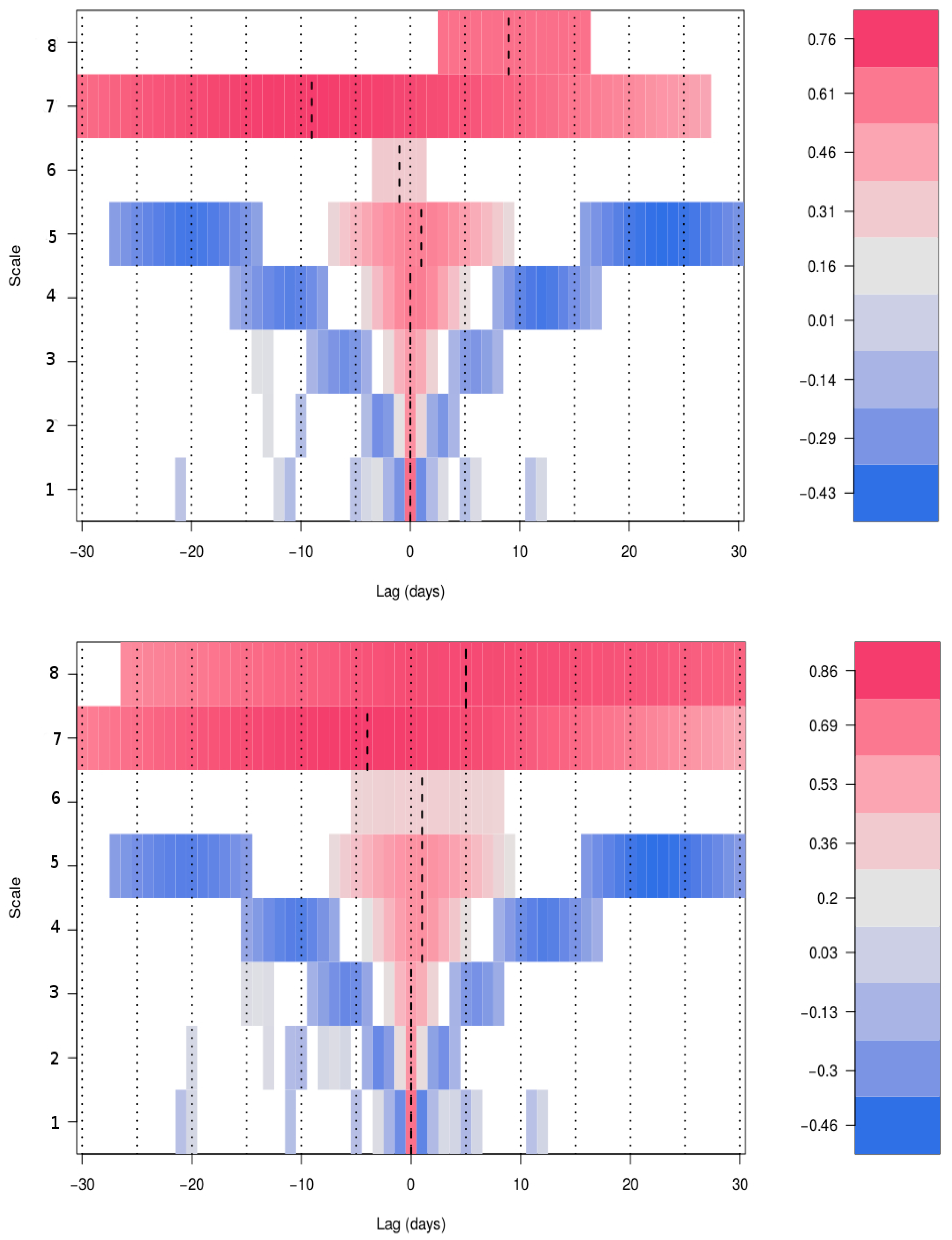
The wavelet cross-correlation between long-term futures prices estimated by a stochastic model and spot prices (Figure 5) shows a high degree of correlation (from 0.46 to 0.76) for all the wavelet scales except for scale six (we so not discuss the results for this scale because there are few statistically significant wavelet correlation coefficients), where the correlation is relatively low (0.30). The maximum wavelet correlations for the first four wavelet scales (from intra-week to monthly scale) take place at lag-0, indicating that futures (spots) do not lead or lag spots (futures). At this point it is important to note that for wavelet scale four and for the price of the future with the longest maturity on that day (Figure 5) the wavelet correlation values show an asymmetry with respect to lag-0 (the maximum correlation takes place at lag-1). This means that futures lead spot prices on a monthly scale. Indeed, there are other wavelet scales (from 5 to 8, for both modeled and non-modeled futures (Figure 5)) that show asymmetries one with another. However, the most noticeable asymmetry appears in scale seven (biannual scale), which can be interpreted as one leading to the other but it cannot be determined which is the leader. Furthermore, one should be cautions when applying the wavelet cross-correlation methodology because although it does give a clue to potential lead-lag relationships it does not include an estimation of causality. For this reason, it is necessary to apply some sort of causality test to the wavelet decomposition of the time series under analysis to corroborate these guesses—these analyses are presented and discussed in the following paragraphs.

Table 6. Non-linear Granger causality test (MODWT decomposition).

(a) Futures * Do Not Cause Spot Prices			Spot Prices Do Not Cause Futures *
Wavelet Scale	T Statistics	p-Value	T Statistics	p-Value
1	2.747	0.0030	2.637	0.0042
2	3.245	0.0006	1.996	0.0229
3	2.777	0.0027	2.359	0.0092
4	2.806	0.0025	1.501	0.0667
5	0.961	0.1683	2.546	0.0054
6	1.899	0.0288	1.017	0.1545
7	2.025	0.0214	1.914	0.0278
8	1.746	0.0404	3.520	0.0002
(b) Futures* Do Not Cause Spot Prices			Spot Prices Do Not Cause Futures *
Wavelet Scale	T Statistics	p-Value	T Statistics	p-Value
1	3.672	0.0001	3.050	0.0011
2	3.926	0.0000	1.658	0.0486
3	3.255	0.0006	2.900	0.0019
4	2.939	0.0016	1.205	0.1141
5	1.507	0.0659	2.127	0.0167
6	1.566	0.0587	1.192	0.1166
7	1.766	0.0387	2.417	0.0078
8	−1.590	0.9441	3.196	0.0007

Note:* indicates Long-Term Futures Obtained by the Stochastic Model.

provides the non-linear Granger causality test between the (modeled and not modeled) futures and spot prices for the MODWT decomposition of this data set. The first noteworthy result is that 4 wavelet scales (one, two, three, and seven) out of 8 show bidirectional causality (note that for scales six and eight—modeled future prices—the number of wavelet coefficients is too low to run the causality test properly; Figure C1, Appendix C). These wavelet scales are related to day-periods that range from intraweek to fortnightly, and one longer scale (seven) which is associated with a biannual day-period. These results are robust due to the fact that bidirectional causality is found for both futures (the price of the future with the longest maturity on that day and the futures prices obtained by means of the stochastic model). On the other hand, there exists a unidirectional causality in the scales four (monthly scale) and five (monthly and quarterly scale), running from futures (both modeled and not modeled) to spot prices and from spot to futures (both modeled and not modeled) prices, respectively. These means that for monthly scale, futures lead spot prices whereas for monthly and quarterly scales spots prices lead futures (both modeled and not modeled)

Our causality test results between the futures and spot prices are in fairly close agreement with Alzahrani et al. [15], although our sample is larger than that analyzed by Alzahrani et al. (we use 24 February 2006–2 April 2016 and they use 20 February 2003–19 April 2011) and the causality tests are not exactly the same. We use the test proposed by Diks and Panchenko [16] whereas Alzahrani et al. use a modified version of the test proposed by Baek and Brock [34]. Alzahrani et al. [15], unlike our work, find bidirectional causality for all wavelet scales (from one to eight). However, Alzahrani et al. [15] apply the causality test to the residuals of the VAR models fitted to the future and spot prices and use daily future prices as well as futures contracts with different maturity periods (one, two, three, and four months). On the other hand, the nonlinear causality test used by Alzahrani et al. tends to detect causality too often (Shu and Zhang [42]) and ours is a little conservative (Wolski and Diks [43], Chiou-Wei et al. [44]). Therefore, we do not expect our results to be identical to those of [15].

The bidirectional causality in the wavelet decomposition of crude oil futures and spot prices suggests that spot and futures prices react concurrently to new information, i.e., neither market leads the other in terms of price discovery, at least for intraweek, weekly, fortnightly, and biannual scales. Thus, there is no arbitrage opportunity between these markets for these time horizons. The most plausible explanation for why we find a not bidirectional causality between futures and spot prices for the monthly and quarterly scales may be that for the monthly scale nonlinear arbitrage activity (e.g., structural breaks, regime shifts between backwardation and contango, extreme volatility, etc. such as was suggested by diverse authors e.g., Wang and Wu [45]; Savit [33]; Wilson et al. [46]; among others. As we can see, all these characteristics can be observed in Figure 3 and Figure D1 and Table 3) is very low and the change in fundamentals supporting market condition switching is not completed within a one month period. That is, the effects of these factors which can result in the nonlinearity explanation for why oil market are weaker (Wang and Wu [45]), and for this reason the non-linear Granger causality test is not able to detect bidirectional causalities for the monthly and quarterly scales.

4. Conclusions

The crude oil spot price is a fundamental variable for the worldwide economy, and the WTI Spot price is one of the most widely used indexes. No less important are crude oil futures prices. It is well known that both prices are affected by fundamental and transitory factors. One fundamental factor is tight production, while transitory factors such as periods of very cold weather can mainly affect spot prices. Many energy intensive sectors such as transport, refineries, energy-intensive industries and others use the spot and futures prices to make decisions on production and/or investment. Therefore, both spot and futures prices and indeed the interrelationship between them are relevant for the economy. For instance, the lead-lag relationship between crude oil spot and futures markets is a debatable issue, as can be corroborated in the many publications on this topic since the seminal 1999 paper by Silvapulle and Moosa [3].

In this paper we propose for the first time the use of a stochastic model (Abadie and Chamorro [18]) to estimate long-term futures in order to study the relationships between futures and spot prices for different time-scales (short, medium, and long-term scales) using a novel wavelet correlation graphical tool (Polanco-Martínez and Fernández-Macho [17]) and a nonlinear causality test. In order to obtain the long-term future prices, which are a fundamental variable for investment decisions, we calibrate a stochastic model of crude oil prices using market quotes.

Our findings suggest that for the period studied (from 24 February 2006–2 April 2016) the spot and long-term futures prices show bidirectional causality for intraweek, weekly, fortnightly, and biannual scales, thus indicating that the two markets react simultaneously to new information on those time scales. On the other hand, for monthly scale futures lead spot prices whereas for monthly-quaterly scale spots pries lead futures. Our results confirm quite well the findings of Silvapulle and Moosa [3]; Bekiros and Diks [6]; Alzahrani et al. [15]; Chang and Lee [12], but we highlight the use of a stochastic model to obtain long-term futures prices.

References

1. Deng, S.; Sakurai, A. Crude oil spot price forecasting based on multiple crude oil markets and timeframes. Energies 2014, 7, 2761–2779. [Google Scholar] [CrossRef]
2. Knittel, C.R.; Pindyck, R.S. The simple economics of commodity price speculation. Am. Econ. J. 2016, 8, 85–110. [Google Scholar] [CrossRef]
3. Silvapulle, P.; Moosa, I.A. The relationship between spot and futures prices: Evidence from the crude oil market. J. Futures Markets 1999, 19, 175–193. [Google Scholar] [CrossRef]
4. Kaufmann, R.K.; Ullman, B. Oil prices, speculation, and fundamentals: Interpreting causal relations among spot and futures prices. Energy Econ. 2009, 31, 550–558. [Google Scholar] [CrossRef]
5. Hammoudeh, S.; Li, H.; Jeon, B. Causality and volatility spillovers among petroleum prices of WTI, gasoline and heating oil in different locations. N. Am. J. Econ. Financ. 2003, 14, 89–114. [Google Scholar] [CrossRef]
6. Bekiros, S.D.; Diks, C.G. The relationship between crude oil spot and futures prices: Cointegration, linear and nonlinear causality. Energy Econ. 2008, 30, 2673–2685. [Google Scholar] [CrossRef]
7. Maslyuk, S.; Smyth, R. Unit root properties of crude oil spot and futures prices. Energy Pol. 2008, 36, 2591–2600. [Google Scholar] [CrossRef]
8. Lee, S.H. International transmission of stock market movements: A wavelet analysis. Appl. Econ. Lett. 2004, 11, 197–201. [Google Scholar]
9. Yousefi, S.; Weinreich, I.; Reinarz, D. Wavelet-based prediction of oil prices. Chaos Solitons Fractals 2005, 25, 265–275. [Google Scholar] [CrossRef]
10. Naccache, T. Oil price cycles and wavelets. Energy Econ. 2011, 33, 338–352. [Google Scholar] [CrossRef]
11. Reboredo, J.C.; Rivera-Castro, M.A. Wavelet-based evidence of the impact of oil prices on stock returns. Int. Rev. Econ. Financ. 2014, 29, 145–176. [Google Scholar] [CrossRef]
12. Chang, C.P.; Lee, C.C. Do oil spot and futures prices move together? Energy Econ. 2015, 50, 379–390. [Google Scholar] [CrossRef]
13. Gençay, R.; Selçuk, F.; Whitcher, B.J. An Introduction to Wavelets and Other Filtering Methods in Finance and Economics; Academic Press: San Diego, CA, USA, 2001. [Google Scholar]
14. Percival, D.B.; Walden, A.T. Wavelet Methods for Time Series Analysis; Cambridge University Press: Cambridge, UK, 2006. [Google Scholar]
15. Alzahrani, M.; Masih, M.; Al-Titi, O. Linear and non-linear Granger causality between oil spot and futures prices: A wavelet based test. J. Int. Money Financ. 2014, 48, 175–201. [Google Scholar] [CrossRef]
16. Diks, C.; Panchenko, V. A new statistic and practical guidelines for nonparametric Granger causality testing. J. Econ. Dyn. Control 2006, 30, 1647–1669. [Google Scholar] [CrossRef]
17. Polanco-Martinez, J.M.; Fernández-Macho, F.J. Package W2CWM2C: Description, Features, and Applications. Comput. Sci. Eng. 2014, 16, 68–78. [Google Scholar] [CrossRef]
18. Abadie, L.M.; Chamorro, J.M. Investments in Energy Assets under Uncertainty; Springer: London, UK, 2013. [Google Scholar]
19. Jarque, C.M.; Bera, A.K. Efficient tests for normality, homoscedasticity and serial independence of regression residuals. Econ. Lett. 1980, 6, 255–259. [Google Scholar] [CrossRef]
20. Trapletti, A.; Hornik, K. Tseries: Time Series Analysis and Computational Finance. R Package Version 0.10-34. 2015. Available online: http://CRAN.R-project.org/package=tseries (accessed on 20 February 2016).
21. Dickey, D.A.; Fuller, W.A. Distribution of the estimators for autoregressive time series with a unit root. J. Am. Stat. Assoc. 1979, 74, 427–431. [Google Scholar] [CrossRef]
22. Percival, D.B.; Mofjeld, H.O. Analysis of subtidal coastal sea level fluctuations using wavelets. J. Am. Stat. Assoc. 1997, 92, 868–880. [Google Scholar] [CrossRef]
23. Gallegati, M. Wavelet analysis of stock returns and aggregate economic activity. Comput. Stat. Data Anal. 2008, 52, 3061–3074. [Google Scholar] [CrossRef]
24. Ramsey, J.B. The contribution of wavelets to the analysis of economic and financial data. Philos. Trans. R. Soc. Lond. A 1999, 357, 2593–2606. [Google Scholar] [CrossRef]
25. Benhmad, F. Modeling nonlinear Granger causality between the oil price and US dollar: A wavelet based approach. Econ. Model. 2012, 29, 1505–1514. [Google Scholar] [CrossRef]
26. Tonn, V.L.; Li, H.C.; McCarthy, J. Wavelet domain correlation between the futures prices of natural gas and oil. Q. Rev. Econ. Financ. 2010, 50, 408–414. [Google Scholar] [CrossRef]
27. Papaioannou, G.P.; Dikaiakos, C.; Evangelidis, G.; Papaioannou, P.G.; Georgiadis, D.S. Co-Movement Analysis of Italian and Greek Electricity Market Wholesale Prices by Using a Wavelet Approach. Energies 2015, 8, 11770–11799. [Google Scholar] [CrossRef]
28. Aguiar-Conraria, L.; Soares, M.J. Oil and the macroeconomy: Using wavelets to analyze old issues. Empir. Econ. 2011, 40, 645–655. [Google Scholar] [CrossRef] [Green Version]
29. Daubechies, I. Ten lectures on wavelets. Soc. Ind. Math. 1992, 93, 1671. [Google Scholar]
30. Whitcher, B. Waveslim: Basic Wavelet Routines for One-, Two- and Three-Dimensional Signal Processing. R Package Version 1.7.5. 2015. Available online: http://CRAN.R-project.org/package=waveslim (accessed on 1 September 2016).
31. Polanco-Martínez, J.M. W2CWM2C: A Graphical Tool for Wavelet (Cross) Correlation and Wavelet Multiple (Cross) Correlation Analysis. R Package Version 2.0. 2015. Available online: http://CRAN.R-project.org/package=W2CWM2C (accessed on 10 May 2015).
32. Whitcher, B.; Guttorp, P.; Percival, D.B. Wavelet analysis of covariance with application to atmospheric time series. J. Geophys. Res. 2000, 105, 941–962. [Google Scholar] [CrossRef]
33. Savit, R. When random is not random: An introduction to chaos in market prices. J. Futures Markets 1998, 8, 271–290. [Google Scholar] [CrossRef]
34. Baek, E.; Brock, W. A General Test for Non-linear Granger Causality: Bivariate Model Working Paper; University of Wisconsin: Madison, WI, USA, 1992. [Google Scholar]
35. Hiemstra, C.; Jones, J.D. Testing for linear and nonlinear Granger causality in the stock price-volume relation. J. Financ. 1994, 49, 1639–1664. [Google Scholar] [CrossRef]
36. Bell, D.; Kay, J.; Malley, J. A non-parametric approach to non-linear causality testing. Econ. Lett. 1996, 51, 7–18. [Google Scholar] [CrossRef]
37. Su, L.; White, H. A nonparametric Hellinger metric test for conditional independence. Econ. Theory 2008, 24, 829–864. [Google Scholar] [CrossRef]
38. Diks, C.; Panchenko, V. A note on the Hiemstra-Jones test for Granger non-causality. Stud. Nonlinear Dyn. Econ. 2005, 9, 1–7. [Google Scholar] [CrossRef]
39. Panchenko, V. Code for T Test Statistics for Granger Causality Test in C. 2005. Available online: http://research.economics.unsw.edu.au/vpanchenko/software/2006_GC_JEDC_c_and_exe_code.zip (accessed on 15 July 2016).
40. Toda, H.; Yamamoto, T. Statistical inference in vector autoregressions with possibly integrated processes. J. Econ. 1995, 66, 225–250. [Google Scholar] [CrossRef]
41. Pfeiffer, C. Toda-Yamamoto Implementation in R. 2012. Available online: http://www.christophpfeiffer.org/2012/11/07/toda-yamamoto-implementation-in-r/ (accessed on 5 November 2016).
42. Zhang, S.; Shu, J.; Zhang, J.E. Causality in the VIX futures market. J. Futures Markets 2012, 32, 24–46. [Google Scholar]
43. Wolski, M.; Diks, C. Data sharpening in practice: An application to nonlinear Granger causality. Aenorm 2013, 21, 19–21. [Google Scholar]
44. Chiou-Wei, S.Z.; Ching-Fu, C.; Zhen, Z. Economic growth and energy consumption revisited—Evidence from linear and nonlinear Granger causality. Energy Econ. 2008, 30, 3063–3076. [Google Scholar] [CrossRef]
45. Wang, Y.; Wu, C. Are crude oil spot and futures prices cointegrated? Not always! Econ. Model. 2013, 33, 641–650. [Google Scholar] [CrossRef]
46. Wilson, B.; Aggarwal, R.; Inclan, C. Detecting volatility changes across the oil sector. J. Future Markets 1996, 16, 313–330. [Google Scholar] [CrossRef]
47. Brennan, M.; Schwartz, E. Evaluating Natural Resource Investments. J. Bus. 1985, 58, 135–157. [Google Scholar] [CrossRef]
48. McDonald, R.L.; Siegel, D.R. Investment and the valuation of Firms when there is an option to shut down. Int. Econ. Rev. 1985, 26, 331–349. [Google Scholar] [CrossRef]
49. Bjerksund, P.; Ekern, S. Contingent Claims Evaluation of Mean-Reverting Cash Flows in Shipping. In Real Options in Capital Investment: Models, Strategies, and Applicationse, 1st ed.; Trigeorgis, L., Ed.; Praeger: Westport, CT, USA, 1995; pp. 207–219. [Google Scholar]
50. Schwartz, E.S. The stochastic behavior of commodity prices: Implications for valuation and hedging. J. Financ. 1997, 52, 923–973. [Google Scholar] [CrossRef]
51. Pilipovic, D. Energy Risk: Valuing and Managing Energy Derivatives, 2nd ed.; McGraw Hill: New York, NY, USA, 2007. [Google Scholar]
52. Abadie, L.M.; Chamorro, J.M. Monte Carlo valuation of natural gas investments. Rev. Financ. Econ. 2009, 18, 10–22. [Google Scholar] [CrossRef]
53. Abadie, L.M.; Galarraga, I.; Rübbelke, D. Evaluation of two alternative carbon capture and storage technologies: A stochastic model. Environ. Model. Softw. 2014, 54, 182–195. [Google Scholar] [CrossRef]
54. Abadie, L.M.; Chamorro, J.M. Revenue Risk of U.S. Tight-Oil Firms. Energies 2016, 9, 848. [Google Scholar] [CrossRef]
55. Zeileis, A.; Kleiber, C.; Krämer, W.; Hornik, K. Testing and dating of structural changes in practice. Comput. Stat. Data Anal. 2003, 44, 109–123. [Google Scholar] [CrossRef]
56. Zeileis, A.; Leisch, F.; Hornik, K.; Kleiber, C.; Hansen, B.; Merkle, E.C. Strucchange: Testing, Monitoring, and Dating Structural Changes. R Package Version 1.5-1. 2015. Available online: http://CRAN.R-project.org/package=strucchange (accessed on 1 March 2016).
Figure 1. WTI Futures Prices term structure (2 April 2016). Source: our own calculations with ICE Futures Prices.
Energies 09 01089 g001
Figure 2. Volatility of returns on contracts with nearest maturity. Source: Our own calculations with ICE futures prices.
Energies 09 01089 g002
Figure 3. WTI spot and futures prices (obtained as the longest maturities and estimated by a stochastic model) covering the time interval from 24 February 2006 to 2 April 2016 and where each time series contain 2571 elements. Source: own work with spot price data from US Energy Information Administration (EIA) and Last Futures Price from Intercontinental Exchange (ICE).
Energies 09 01089 g003
Figure 4. Cross-correlation between long-term futures prices estimated by a stochastic model and spot prices (top), and futures prices obtained as the longest maturity on that day and spot prices (bottom).
Energies 09 01089 g004
Figure 5. Wavelet cross-correlation for the long-term futures prices estimated by a stochastic model and spot prices (top) and futures prices obtained as the longest maturity on that day and spot prices (bottom).
Energies 09 01089 g005