Sensorless Control of Interior Permanent Magnet Synchronous Motor in Low-Speed Region Using Novel Adaptive Filter

Abstract

This paper presents a novel position and speed estimation method for low-speed sensorless control of interior permanent-magnet synchronous machines (IPMSMs). The parameter design of the position and speed estimator is based on the sampled current rather than the motor electrical parameters. The proposed method not only simplifies the parameter design, it enables the estimator to work normally even in the condition that the electrical parameters are uncertain or varied. The adaptive filters are adopted to extract the desired high frequency current. The structure and corresponding transfer function are analyzed. To address the shortage of insufficient stop-band attenuation, the structure of the adaptive filter is modified to provide suitable bandwidth and stop-band attenuation simultaneously. The effectiveness of the proposed sensorless control strategy has been verified by simulations and experiments.

1. Introduction

Interior permanent-magnet synchronous machines (IPMSMs) are widely employed in high-performance applications due to their high power density and efficiency. For vector control of IPMSMs, it is important to acquire the accurate rotor position and velocity. However, the use of the speed sensor means high cost, increased complexity and reduced reliability [1]. Meanwhile, the sensorless control can provide backup control in sensor-based IPMSMs drives during the failure of the speed sensor. Therefore, the sensorless control strategies of IPMSMs have developed rapidly is the last two decades.

The sensorless control strategies can be roughly divided into two categories: fundamental excitation methods [2,3] and signal injection methods [4]. In the fundamental excitation methods, the rotor position is obtained by estimating the back electromotive force (EMF) based on the motor mathematical model. Observer methods [5,6,7,8] and the extended Kalman filtering method [9,10] are used to extract the back EMF information. The parameter estimation scheme is combined with the position observer to guarantee the accuracy of the motor mathematical model, even if the electrical parameters are influenced by the temperature factor [11].

The fundamental excitation methods are effective in the medium to high speed region. However, at the low speed region, these methods fail to operate because the back EMF information is too small. Rather than the back EMF, the signal injection methods are based on the anisotropic properties of IPMSMs, caused either by the inherent saliency due to the machine geometry [12,13] or by the saturation of the stator iron [14]. Therefore, these methods can be utilized to estimate speed and position information in the low speed region, including zero speed. Two kinds of carrier signals, revolving high frequency carrier signal and pulsating high frequency carrier signal, are usually used to estimate the rotor speed and position [15,16,17]; though the form of injected voltage vector differs: the former injects the revolving voltage vector with a higher frequency than the fundamental voltage vector at the two-phase stationary coordinate; the latter injects the pulsating high frequency voltage vector in a specific direction at the two-phase rotating coordinate. They both generate corresponding high frequency carrier current and extract the desired information from it. Meanwhile, they share similar demodulation methods [16]. In usual practice, a band-pass filter is used to obtain the desired high frequency current; a low-pass filter is used to extract the amplitude of the demodulation signal [18]. In [12], a particular demodulation scheme is introduced. Unlike the common demodulation scheme that uses the voltage as the reference signal when extracting the position-related information, the high frequency current itself is used to estimate the rotor speed and position. Because both the position-related information and the reference high frequency current undergo nonlinear distortions of inverters, this demodulation scheme shows the good property of restraining the nonlinear influence.

Regardless of the demodulation schemes mentioned above, the rotor position information is obtained from the high frequency carrier current. The design of the band-pass filter is crucial. On the one hand, it should have a proper bandwidth to ensure the convergence speed. On the other hand, a higher stop-band attenuation is favorable for cutting off the undesired frequency component. A new attempt is introducing the adaptive filter with a neural network structure to the signal processing in the sensorless control scheme. This kind of adaptive filter is introduced in [19] as a noise canceler. In [20], the adaptive filter ensures better dynamic performance and enlarges the working speed range of the sensorless drives. In [21], the adaptive filter is adopt to eliminate the estimation harmonic error caused by the inverter nonlinearities and flux spatial harmonics. Benefiting from its linear network structure, it is convenient to specify the frequency to be canceled or allowed to pass. Additionally, its bandwidth is adjustable by modifying the learning rate of the least mean square (LMS) algorithm or the forgetting factor of the recursive least square (RLS) algorithm. It is noteworthy that the high stop-band attenuation and wide bandwidth cannot be met simultaneously for the adaptive filter. To ensure the convergence speed of the sensorless scheme, the stop-band attenuation is sacrificed. The q-axis stator current is proportional to the electromagnetic torque. When the motor is at load, the desired high frequency current is superimposed on the fundamental q-axis stator current. If the stop-band attenuation is not high enough, the high frequency current filtered by the adaptive filter would be still influenced by the DC offset. If the common demodulation scheme is adopted, the low-pass filter that is used to extract the amplitude of the position-related information acts as a compensator to the low frequency attenuation actually. However, in the demodulation scheme introduced in [12], the high frequency current is used directly for the speed estimation. Therefore, it is necessary to modify the structure of the adaptive filter to enable it to have enough low frequency attenuation.

In addition to the filter selection, the speed and position estimation algorithm is crucial. If the high frequency voltage vector is injected in a specific direction at the two-phase rotating coordinate, the corresponding high frequency current contains the position error information between the real coordinates and the estimated coordinates. Using the principle of the phase-locked loop [22], the speed and position estimation algorithm is derived [23,24]. The algorithm’s major advantage is its tuning convenience. Unlike the trial and error method, the performance of the estimator has a clear relationship with the motor’s electrical parameter. However, on the other hand, the change of the electrical parameters due to the environmental impact would influence the estimator’s performance conversely. This paper presents a Phase Locked Loop (PLL)-type speed and position estimator whose parameter selection is based on the extracted high frequency current rather that the electrical parameters. Therefore, the speed and position estimator proposed is robust against varying parameters. The adaptive filter is adopted to extract the desired high frequency current. In order to coincide with the estimation algorithm, the conventional structure of the adaptive filter is modified to acquire a better low frequency attenuation. The simulation and experiment results verify the effectiveness of the proposed sensorless control scheme.

2. IPMSM Model and PLL-Type Estimator

2.1. IPMSM Model

This paper involves transformation between different coordinates. For convenience, the superscripts ^(S) and ^(R) refer to the stationary coordinates, the real rotor coordinates and the estimated rotor coordinates, respectively. θ refers to the real rotor position. The voltage models in the stationary $\alpha \beta$ coordinates and in the rotating $dq$ coordinates are expressed as:

$${\overrightarrow{u}}^{\left(S\right)}=R·{\overrightarrow{i}}^{\left(S\right)}+\frac{d{\overrightarrow{\psi }}^{\left(S\right)}}{dt}$$

(1)

$${\overrightarrow{u}}^{\left(R\right)}={\overrightarrow{u}}^{\left(S\right)}·e^{-j\theta }=R·{\overrightarrow{i}}^{\left(R\right)}+\frac{d{\overrightarrow{\psi }}^{\left(R\right)}}{dt}+j·\omega ·{\overrightarrow{\psi }}^{\left(R\right)}.$$

(2)

The rotating factor $e^{-j\theta }$ indicates the vector relation between these two coordinates. The vector ${\overrightarrow{\psi }}^{\left(S\right)}$ is the total flux linkage, which has a nonlinear relationship with the current vector ${\overrightarrow{i}}^{\left(S\right)}$. The nonlinear relationship can be expressed in terms of inductance, which is a function of electrical rotor position θ. In the rotating coordinates, the time varying inductance is transformed into constant, shown as:

$$\left[\begin{array}{c}\frac{d{\psi }_d}{dt}\\ \frac{d{\psi }_q}{dt}\end{array}\right]=\left[\begin{array}{cc}{L}_d& L_{dq}\\ L_{qd}& L_q\end{array}\right]\left[\begin{array}{c}\frac{d{i}_d}{dt}\\ \frac{d{i}_q}{dt}\end{array}\right]+\left[\begin{array}{c}\frac{\partial {\psi }_d}{\partial \theta }\\ \frac{\partial {\psi }_q}{\partial \theta }\end{array}\right]\frac{d\theta }{dt}.$$

(3)

For the sake of convenience, the flux linkage distribution is assumed to be perfectly sinusoidal, so the self-inductance terms $L_d$, $L_q$ are taken as constants, and the mutual inductance terms $L_{dq}$, $L_{qd}$, as well as $\frac{d{\overrightarrow{\psi }}^{\left(R\right)}}{d\theta }$ are assumed to be zero. Under these assumptions, the IPMSM model can be expressed in matrix form as:

$$\left[\begin{array}{c}{u}_d\\ u_q\end{array}\right]=\left[\begin{array}{cc}R+p{L}_d& -\omega L_q\\ \omega L_d& R+p{L}_q\end{array}\right]\left[\begin{array}{c}{i}_d\\ i_q\end{array}\right]+\left[\begin{array}{c}0\\ \omega {\lambda }_f\end{array}\right],$$

(4)

where p represents the differential operator and ${\lambda }_f$ represents the permanent-magnet flux linkage.

As to the high frequency model, the injection frequency ${\omega }_c$ is spectrally separated from the fundamental frequency ω. The resistive loss term and the back electromotive force (EMF) term are negligible compared with the derivative of the flux linkage term. The high frequency model of IPMSM can be regarded as a pure inductive load shown as:

$${\overrightarrow{u_c}}^{\left(R\right)}\approx \frac{d{\overrightarrow{\psi }}^{\left(R\right)}}{dt}$$

(5)

$$\left[\begin{array}{c}{u}_{cd}\\ u_{cq}\end{array}\right]\approx \left[\begin{array}{cc}{L}_d& 0\\ 0& L_q\end{array}\right]\left[\begin{array}{c}\frac{d{i}_{cd}}{dt}\\ \frac{d{i}_{cq}}{dt}\end{array}\right].$$

(6)

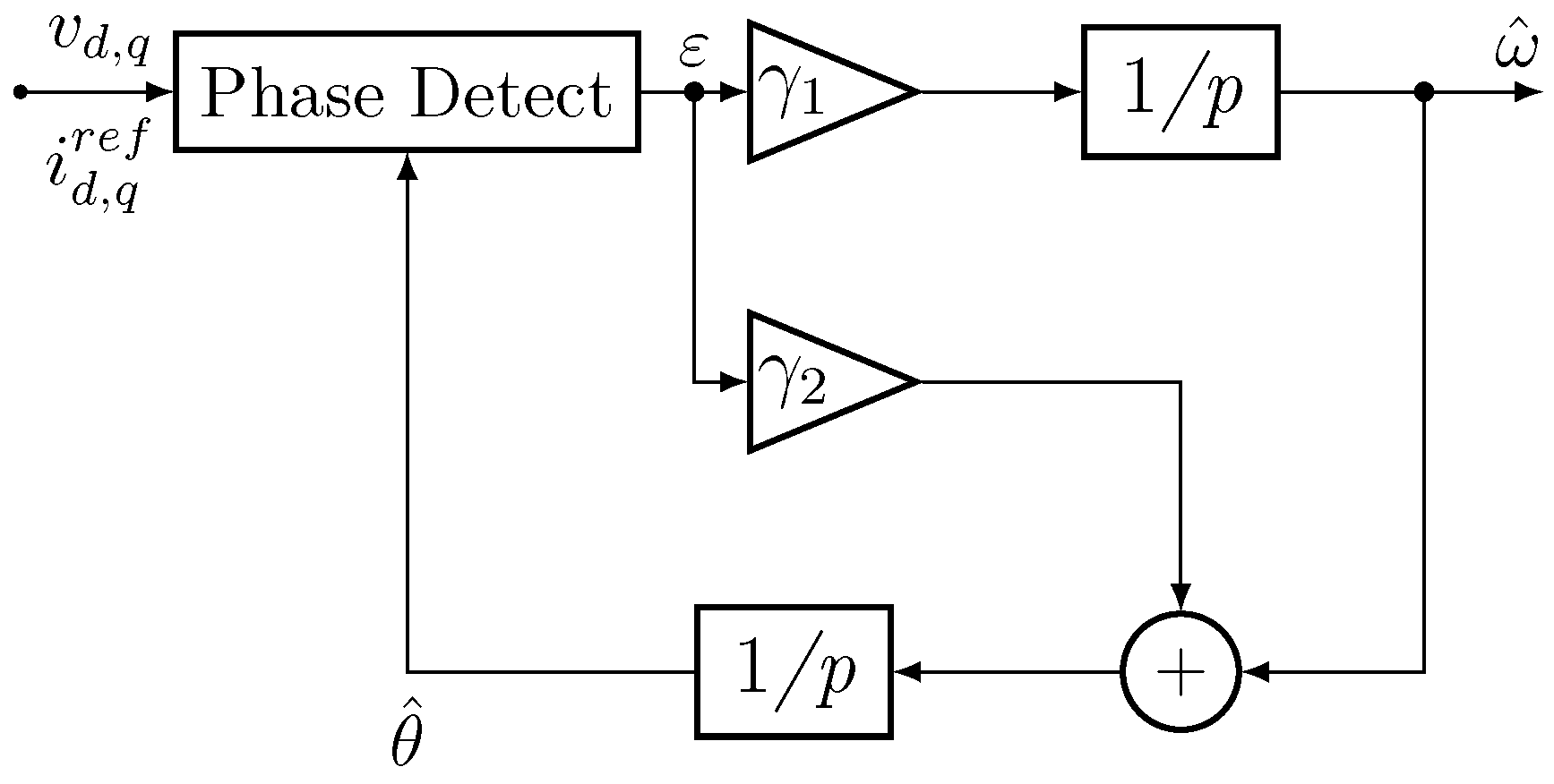
2.2. PLL-Type Estimation Algorithm

The essence of sensorless control is to extract position-related information from sampled current and voltage signals. In the stationary coordinates model of IPMSM, the position information is involved in the EMF term. Direct calculation methods and observer methods are often adopted to obtain the rotor position. However, motor vector control is conducted in the rotating coordinates owing to its decoupling property. In the sensorless control, as the real rotor position is unknown, the position estimation error $\tilde{\theta }=\theta -\widehat{\theta }$, where $\widehat{\theta }$ refers to the estimated rotor position, is bound to exist when the coordinate transformation is conducted, as shown in Figure 1.

If the error signal is defined as:

$$\epsilon =Ksin(\theta -\widehat{\theta }),$$

(7)

where K is the application specific gain, the PLL-type estimation algorithm can be summarized in mathematical form as:

$$\dot{\widehat{\omega }}={\gamma }_1\epsilon$$

(8)

$$\dot{\widehat{\theta }}=\widehat{\omega }+{\gamma }_2\epsilon ,$$

(9)

and in flowchart form as Figure 2. With the error signal calculation corresponding to the phase detecting, the algorithm shares a similar structure with the conventional PLL.

The steady-state and dynamic performances of the PLL-type algorithm are analyzed in detail in [23]. By properly selecting the gain ${\gamma }_1$ and ${\gamma }_2$ as:

$${\gamma }_1=\frac{{\rho }^2}{K}$$

(10)

$${\gamma }_2=\frac{2\rho }{K},$$

(11)

a stable speed and position estimator is acquired, with the dynamic property related to the selection of ρ.

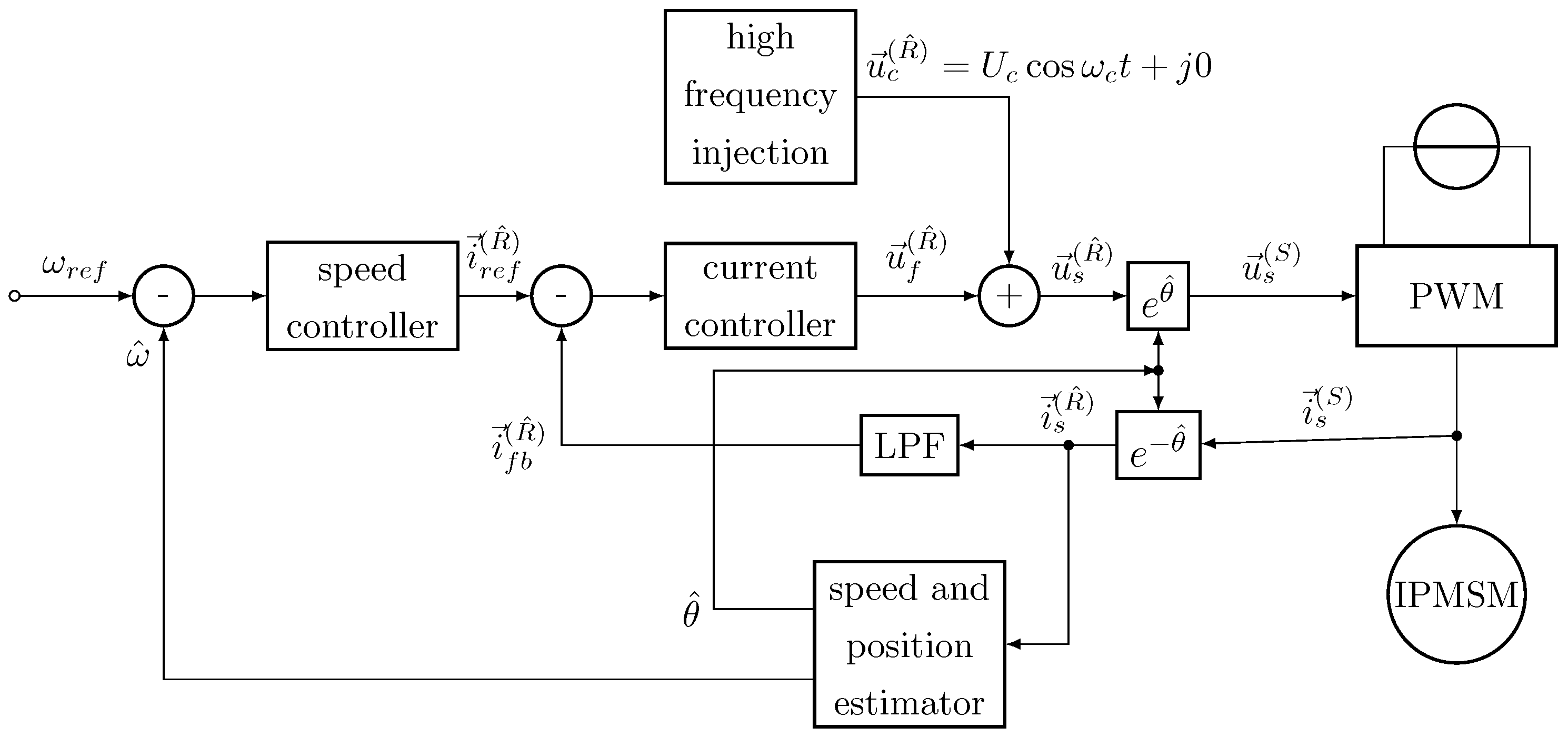
3. Sensorless Control Scheme

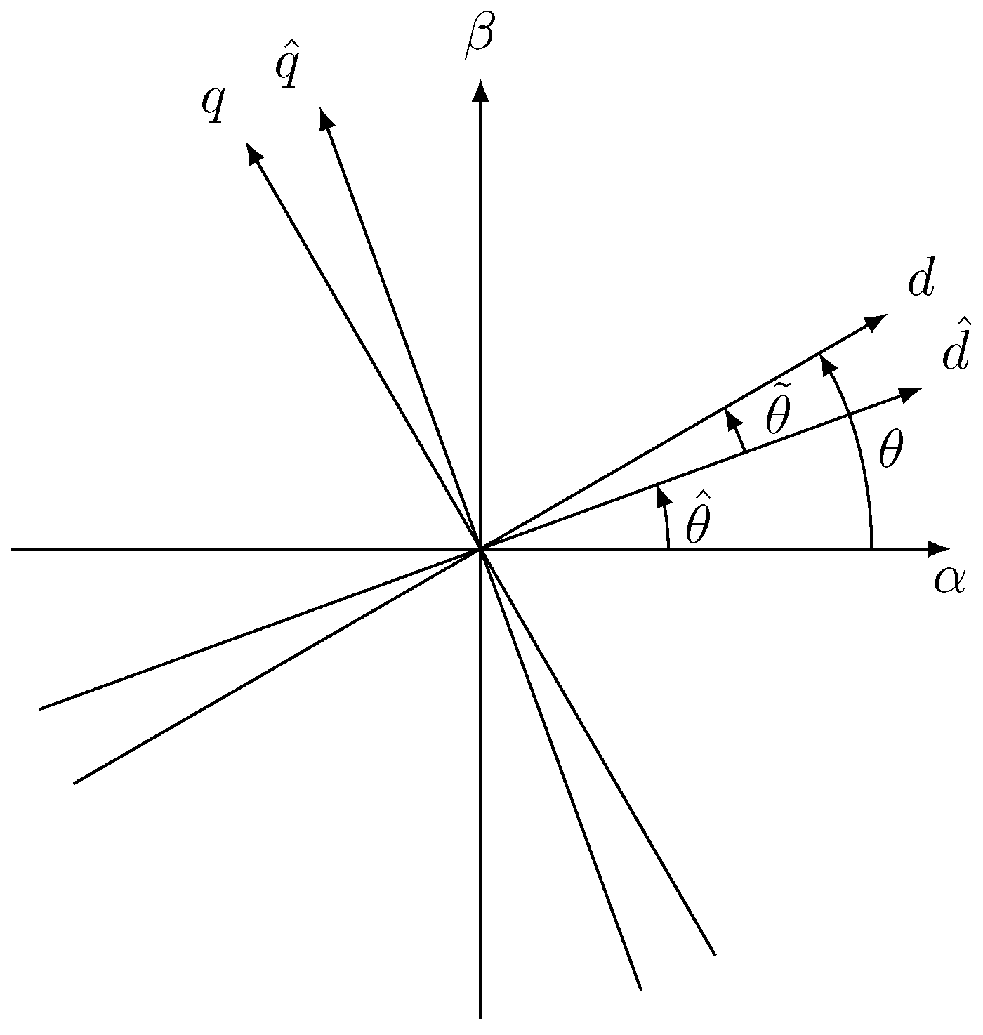
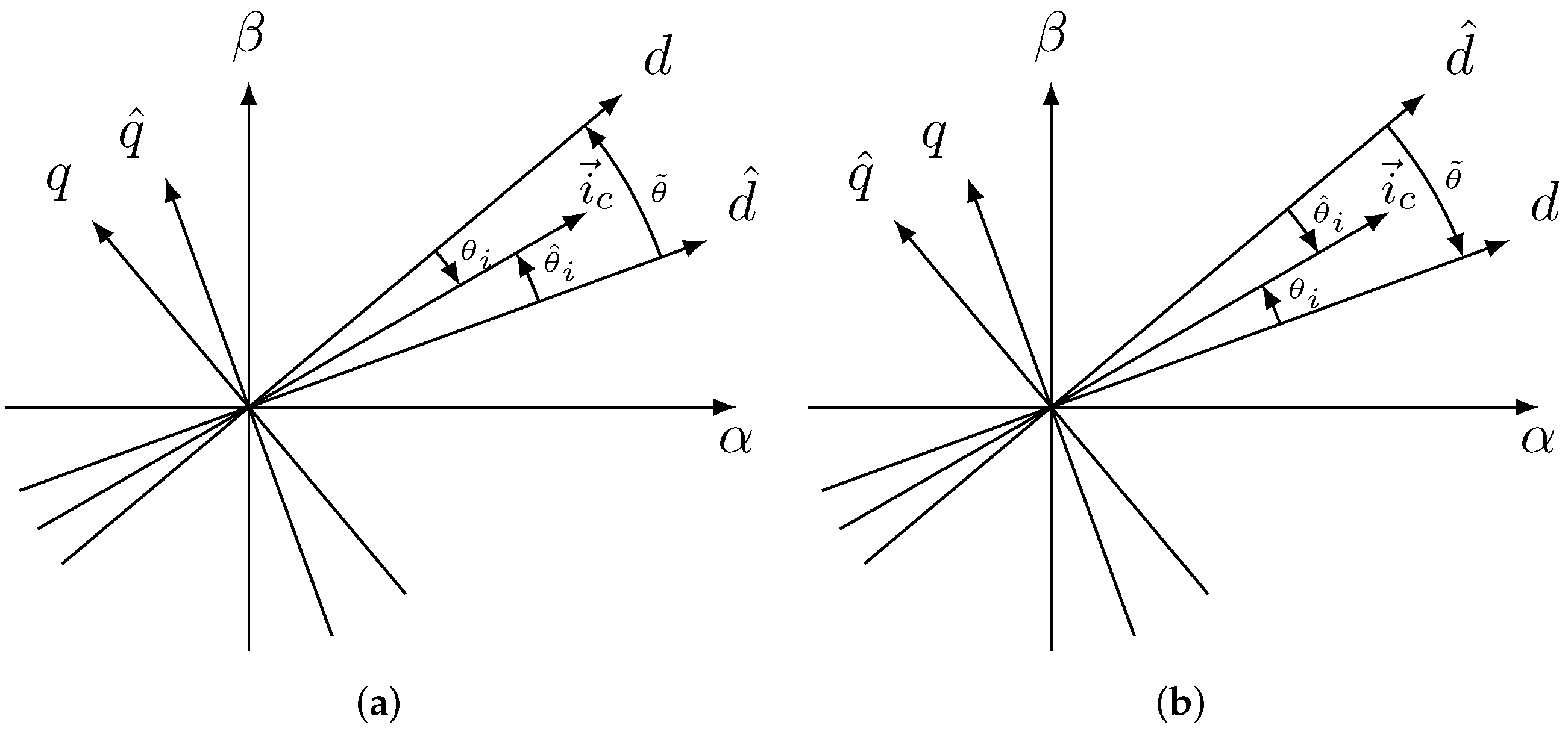
3.1. High Frequency Model Analysis

The overall sensorless control scheme can be expressed as Figure 3 where the subscript _ref represents the current reference given by the speed controller, the subscript _f represents the fundamental part of the electrical variables and the subscript _fb represents the current feedback. The subscript _s represents the values containing both the fundamental part and the high frequency part. As the real rotor coordinates are unknown, a pulsating high frequency voltage as:

$${\overrightarrow{u_c}}^{\left(\widehat{R}\right)}=U_{c}cos{\omega }_{c}t+j0$$

(12)

is injected in the estimated rotor coordinate. Using the position estimation error $\tilde{\theta }$, this voltage can be expressed in the real rotor coordinates as:

$${\overrightarrow{u_c}}^{\left(R\right)}={\overrightarrow{u_c}}^{\left(\widehat{R}\right)}·e^{-j\tilde{\theta }}.$$

(13)

The frequency ${\omega }_c$, which is the frequency of the injected signal, needs enough frequency separation from the fundamental voltage frequency, so that the high frequency current can easily be extracted by filters. The voltage amplitude should be large enough to give a substantial signal-to-noise ratio with the premise that the high frequency current does not affect the normal motor control. In this paper, ${\omega }_c=2\pi ·1000$ rad/s and $U_c=50$ V are selected.

The high frequency current formula:

$$\left[\begin{array}{c}{i}_{cd}\\ i_{cq}\end{array}\right]={\left[\begin{array}{cc}{L}_d& 0\\ 0& L_q\end{array}\right]}^{-1}\left[\begin{array}{c}\int u_{cd}dt\\ \int u_{cq}dt\end{array}\right]$$

(14)

can be deduced from (6) and expressed in vector form as:

$${\overrightarrow{i_c}}^{\left(R\right)}\approx \overrightarrow{{\psi }_c}\left(\frac{1}{L_d}cos\tilde{\theta }-j\frac{1}{L_q}sin\tilde{\theta }\right),$$

(15)

where $\overrightarrow{{\psi }_c}=\frac{U_c}{{\omega }_c}sin{\omega }_{c}t$. In general, the pulsating voltage is injected in the estimated $\widehat{d}$-axis as shown in (12). If the estimated coordinates coincide with the real coordinates, that is $\tilde{\theta }=0$, the corresponding high frequency current only pulsates in the real d-axis; while if $\tilde{\theta }\ne 0$, there is a pulsating current component in the real q-axis. Therefore, the current vector ${\overrightarrow{i_c}}^{\left(R\right)}$ deviates from the real d-axis, as shown in Figure 4.

According to (15), the displacement angle between vector ${\overrightarrow{i}}_c$ and the d-axis can be expressed as:

$${\theta }_i=-atan\left(\frac{L_d}{L_q}tan\tilde{\theta }\right).$$

(16)

From Figure 4, the angle ${\widehat{\theta }}_i=\tilde{\theta }+{\theta }_i$. Additionally, the angle ${\widehat{\theta }}_i$ is the current vector angle in the estimated coordinates. Therefore, ${\widehat{\theta }}_i$ can be expressed as:

$${\widehat{\theta }}_i=\tilde{\theta }-atan\left(\frac{L_d}{L_q}tan\tilde{\theta }\right).$$

(17)

Noticing $L_d\ne L_q$ for IPMSMs, ${\widehat{\theta }}_i=0$ yields $\tilde{\theta }={\theta }_i=0$, which means that the estimated coordinates coincide with the real coordinates.

3.2. Estimator Analysis

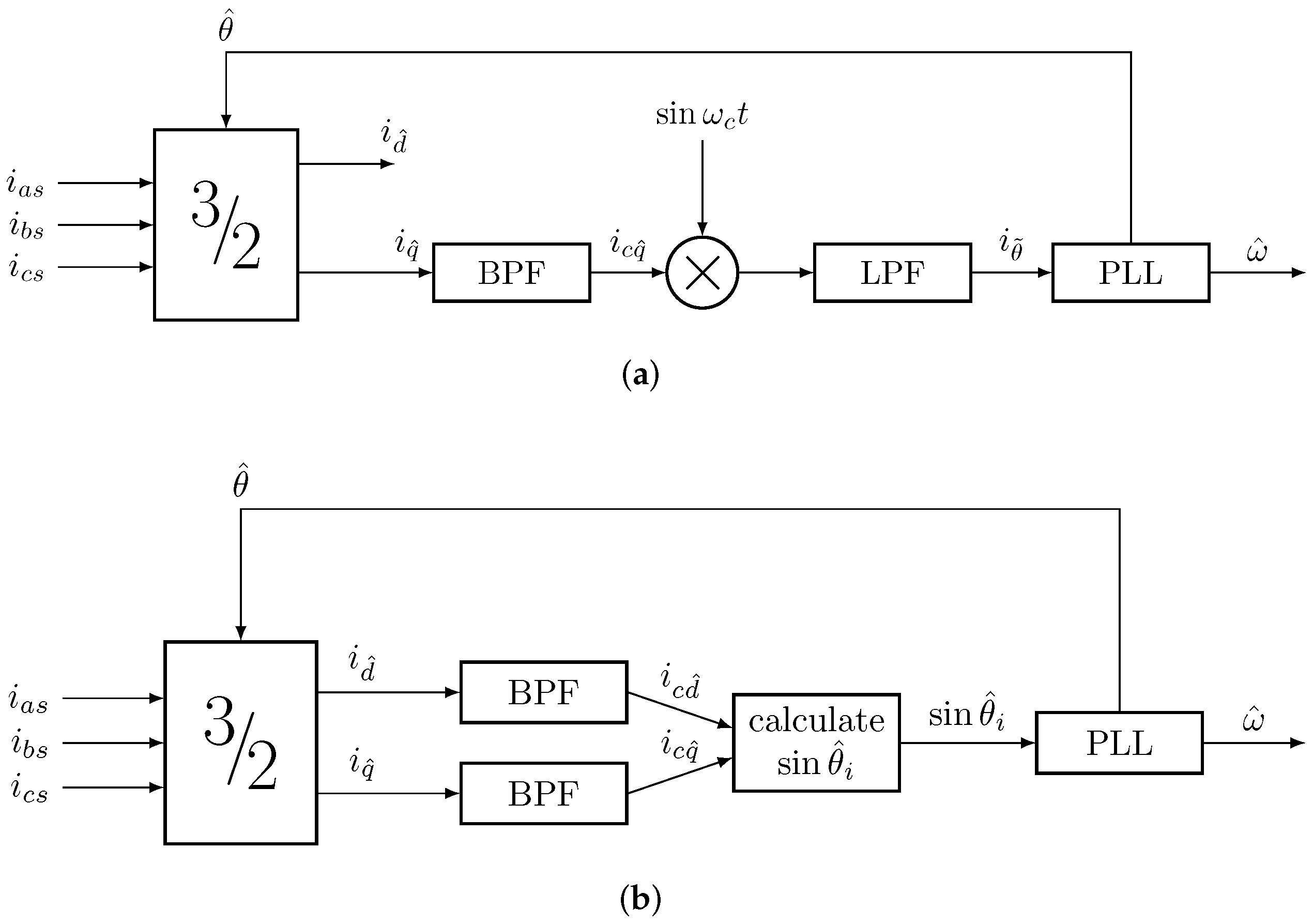
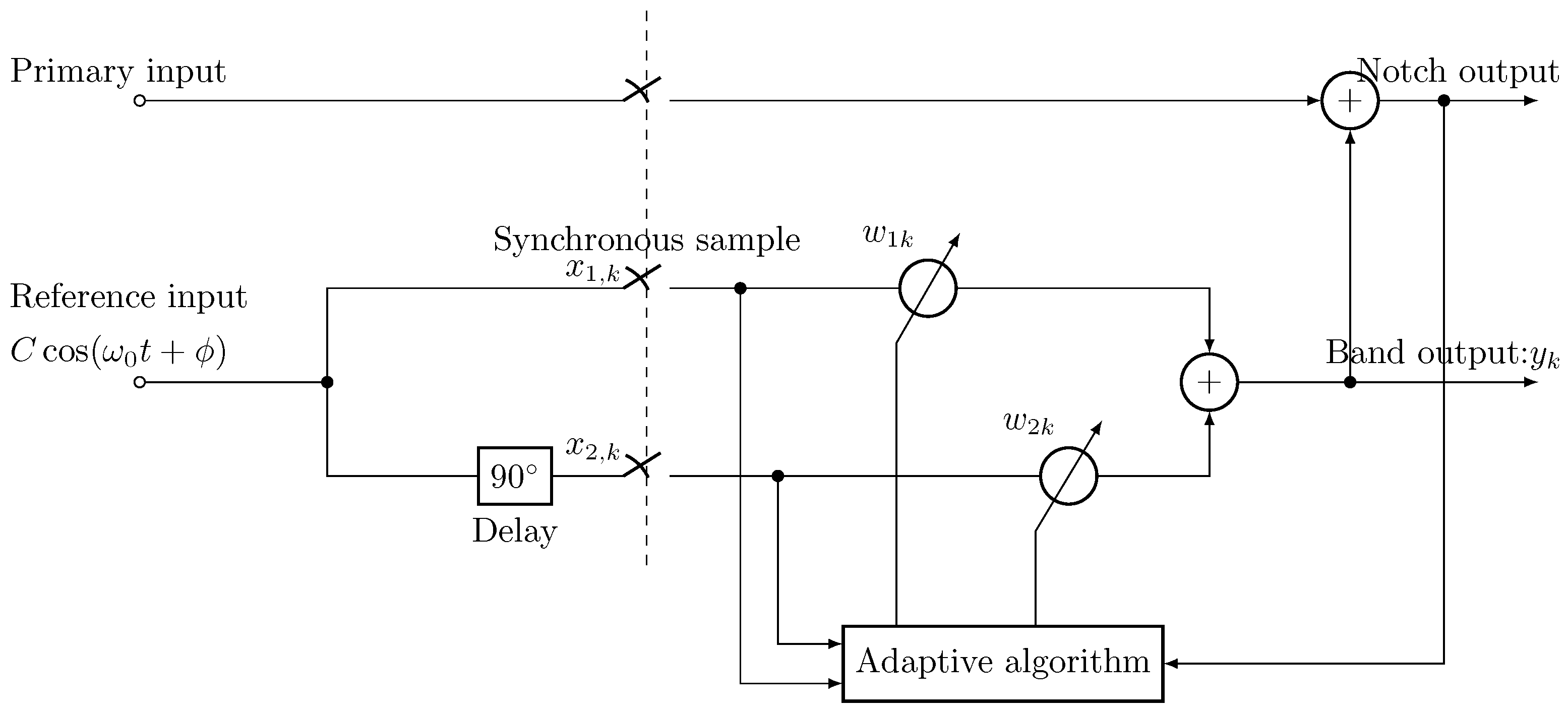
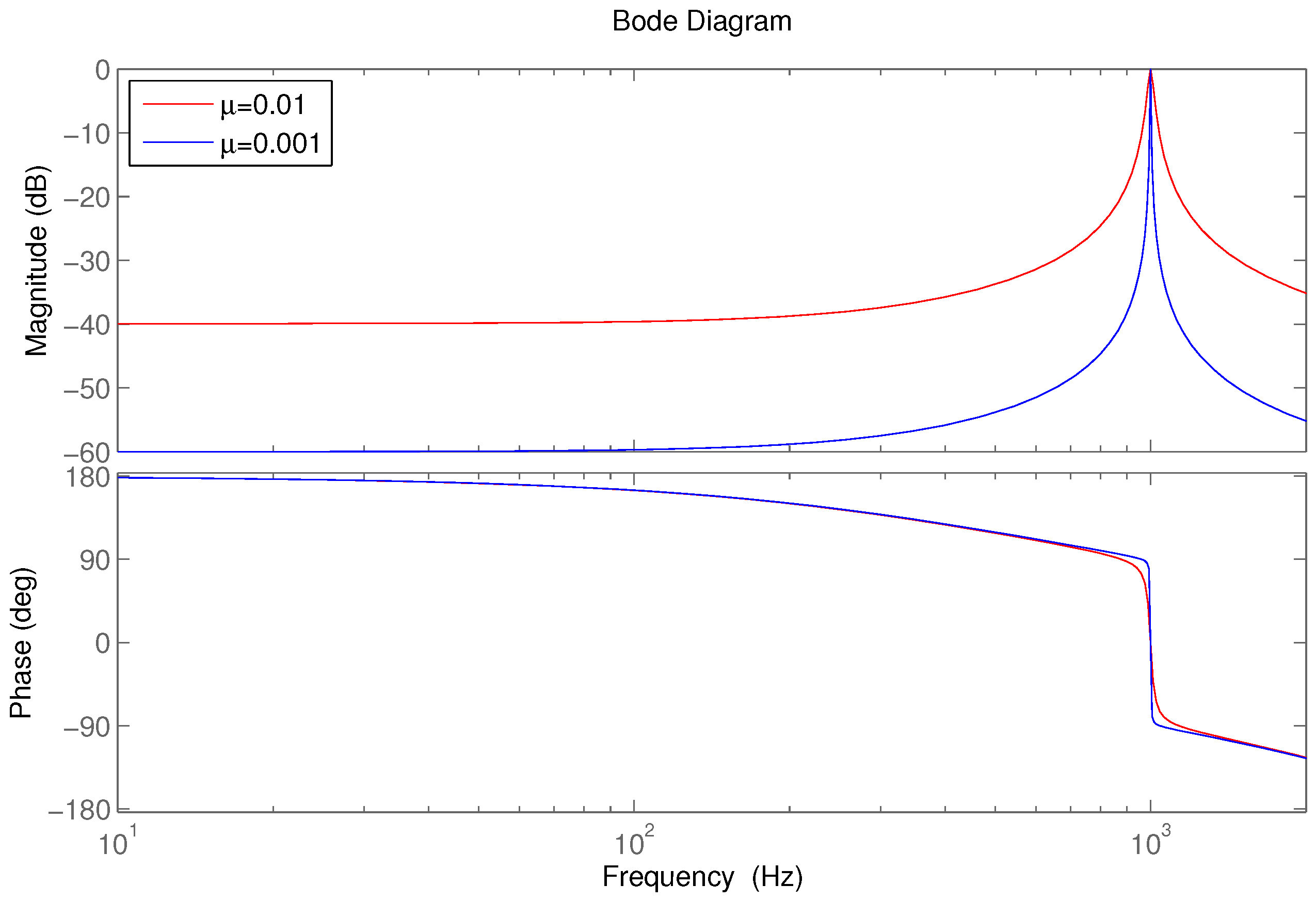
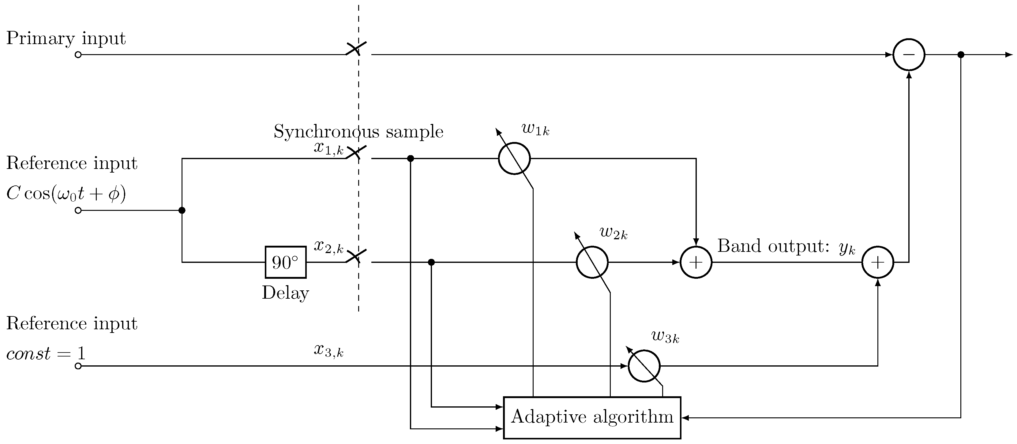
From the control perspective, the rotor position estimation can be achieved either by minimizing the angle $\tilde{\theta }$ or the angle ${\widehat{\theta }}_i$. The PLL-type estimator is suitable for both schemes. The main differences are the signal extraction complexity and the estimator parameters selection. As Figure 5a shows, the $\tilde{\theta }$ related information is contained in $i_{c\widehat{q}}$. In order to obtain the desired information, Band-Pass Filter (BPF) and Low-Pass Filter (LPF) are needed with multiplication operations. The estimator parameters are designed according to the motor’s electrical parameters, for instance $K=\frac{U_c}{{\omega }_c}\frac{L_q-L_d}{4L_q{L}_d}$ is designed in [25].

In this paper, the angle ${\widehat{\theta }}_i$ is used for PLL operation. Referring to Equation (7), the core work focuses on expressing $sin{\widehat{\theta }}_i$ using the high frequency current. In order to acquire the desired information, two identical BPFs are needed to extract the high frequency current $i_{c\widehat{d}}$ and $i_{c\widehat{q}}$, respectively. The current vector ${\overrightarrow{i}}_c$ oscillates in a spacial direction separated from the $\widehat{d}$-axis by angle ${\widehat{\theta }}_i$, as shown in Figure 6. Taking the oscillating current into account, $sin{\widehat{\theta }}_i$ is expressed as:

$$sin{\widehat{\theta }}_i=\frac{i_{c\widehat{q}}}{\sqrt{{\left(i_{c\widehat{d}}\right)}^2+{\left(i_{c\widehat{q}}\right)}^2}}\mathrm{sign}\left(i_{c\widehat{d}}\right).$$

(18)

As shown in Figure 5b, the calculated $sin{\widehat{\theta }}_i$ is then passed to the PLL-type estimator. By minimizing the angle ${\widehat{\theta }}_i$, that is ${\widehat{\theta }}_i\to 0$, the estimated $\widehat{d}$-axis keeps pace with the real rotor position d-axis. The output of the estimator is the angular velocity $\widehat{\omega }$, and the estimated rotor position angle $\widehat{\theta }$ is obtained by integrating $\widehat{\omega }$, as shown in Equations (8) and (9).

The proposed signal extraction method calculates the $sin{\widehat{\theta }}_i$ directly using the sampled high frequency current, which makes the parameter K in (7) equal one. When designing the estimator parameters ${\gamma }_1$ and ${\gamma }_2$, the work is reduced to merely selecting an appropriate parameter ρ that relates to the convergence rate of the estimator. The estimator parameters have no relationship with the motor electrical parameters, which would be likely to change along with the environment. Therefore, the proposed method not only simplifies the parameter design, but also enables the estimator to work normally even in the condition that the motor electrical parameters are uncertain or varied.

4. Adaptive Filter

4.1. Structure of the Adaptive Filter

In the sensorless control scheme, the design of BPF is critical. On the one hand, an adequate stop-band attenuation is necessary to suppress interference. On the other hand, a suitable pass bandwidth is needed to ensure the convergence rate. In [19], the adaptive filter is designed as a notch to attenuate 60-Hz noise in an electrocardiogram (ECG). The similar adaptive filter can be used as BPF, as well [20,21].

The adaptive filter is based on the linear neural network. As compared with the classic fixed-band BPF, the adaptive filter provides an easy way to track the exact frequency by adapting its weights online, and the pass bandwidth can be adjusted. The structure of the adaptive filter is shown in Figure 7. The primary input contains high frequency current, fundamental current and other interference signals. The reference inputs are two orthogonal signals shown as:

$$\begin{array}{c}{x}_{1,k}=Ccos\left(k{\omega }_0+\varphi \right)\hfill \\ x_{2,k}=Csin\left(k{\omega }_0+\varphi \right)\hfill \end{array},$$

(19)

where ${\omega }_0=2\pi f_{0}T$. The reference frequency ${\omega }_0$ is determined at the frequency to cancel or to allow it to pass. The weights $w_{1,k}$ and $w_{2,k}$ are updated according to adaptive algorithms, such as LMS or RLS.

The LMS algorithm is adopted as:

$$\begin{array}{c}{w}_{1,k+1}=w_{1,k}+2\mu {\epsilon }_k{x}_{1,k}\hfill \\ w_{2,k+1}=w_{2,k}+2\mu {\epsilon }_k{x}_{2,k}\hfill \end{array}$$

(20)

$$y_k=x_{1,k}{w}_{1,k}+x_{2,k}{w}_{2,k},$$

(21)

where μ represents the convergence parameter. The linear transfer function for the adaptive filter, from the primary input to the system output, can be described as Figure 8. Having the transfer function of the forward channel, which is expressed as:

$$G_1\left(z\right)=\frac{2\mu C^2\left(zcos{\omega }_0-1\right)}{z^2-2zcos{\omega }_0+1},$$

(22)

the closed-loop transfer function $H\left(z\right)$, from the primary input to the band output, can be obtained as:

$$H\left(z\right)=\frac{2\mu C^2\left(zcos{\omega }_0-1\right)}{z^2-2\left(1-\mu C^2\right)zcos{\omega }_0+1-2\mu C^2}.$$

(23)

Figure 9 shows the locations of poles and zeros when $f_0=1000\mathrm{Hz}$ and ${\omega }_0=\pi /4$. The transfer function has one zero $z_{zero}=1/\cos {\omega }_0$ and two poles as:

$$\begin{array}{c}{z}_{poles}=\left(1-\mu C^2\right)cos{\omega }_0\pm j{\left[\left(1-2\mu C^2\right)-{\left(1-\mu C^2\right)}^2{cos}^2{\omega }_0\right]}^{1/2}\end{array}.$$

(24)

The poles are located inside the unit circle at a radial distance ${\left(1-2\mu C^2\right)}^{1/2}$, approximately equal to $1-\mu C^2$. Additionally, for slow adaptation, which means small values of $\mu C^2$, the angles of the poles are almost identical to ${\omega }_0$ [19]. The distance between the points $z=e^{\pm j{\omega }_0}$ and the corresponding poles, which determine the sharpness of the filter, is approximately equal to $\mu C^2$. The frequency near ${\omega }_0$ is the passband frequency, and the bandwidth shown as:

$$BW=2\mu C^2\mathrm{rad}=\frac{\mu C^2}{\pi T}\mathrm{Hz},$$

(25)

is the length of the arc along the unit circle near ${\omega }_0$.

The magnitude-phase characteristic of $H\left(z\right)$ is shown in Figure 10. Obviously, for the same value of C, a larger value of μ enables a wider bandwidth, but reduces low frequency attenuation, as well. To guarantee a satisfactory convergence rate, the low frequency attenuation has to be sacrificed to ensure sufficient bandwidth. The insufficient attenuation results in a DC bias that cannot be ignored existing along with the desired high frequency signal. As for the specific signal process discussed in Section 3.2, the high frequency current is used directly to calculate $sin{\widehat{\theta }}_i$. The insufficient low frequency attenuation would influence the performance of the estimator undoubtedly. To cope with the proposed signal process, the adaptive filter structure needs to be adjusted to ensure an appropriate bandwidth and a sufficient low frequency attenuation simultaneously.

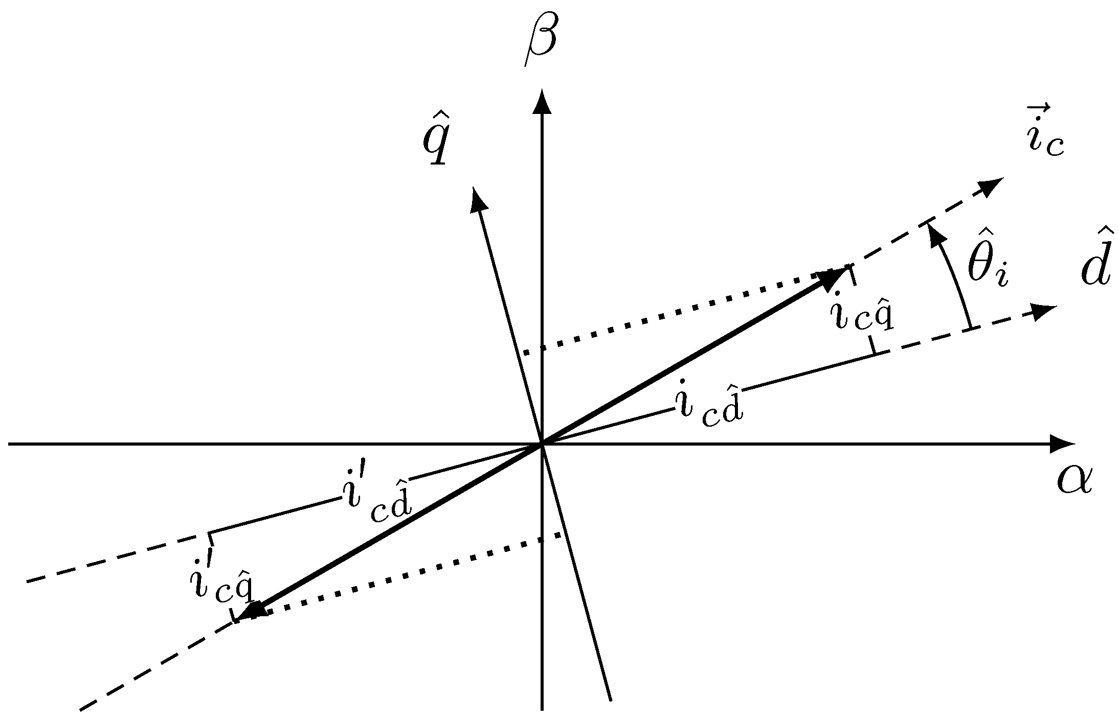
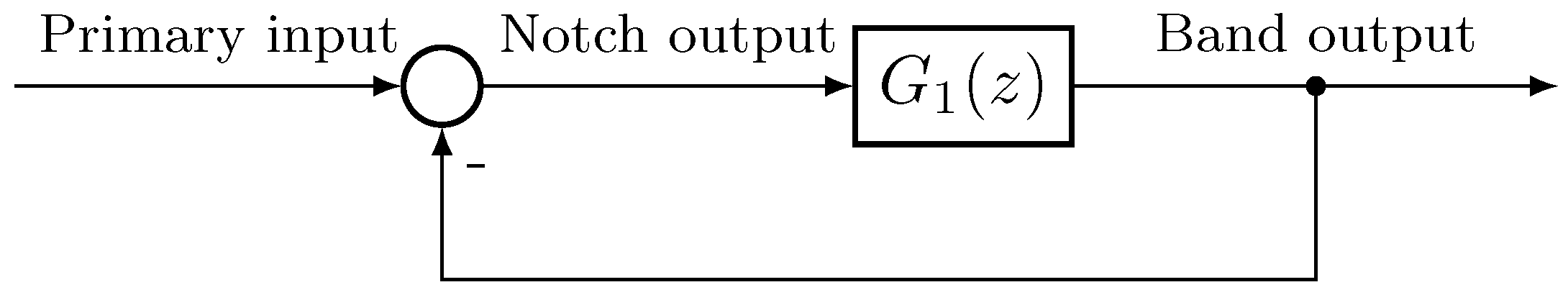
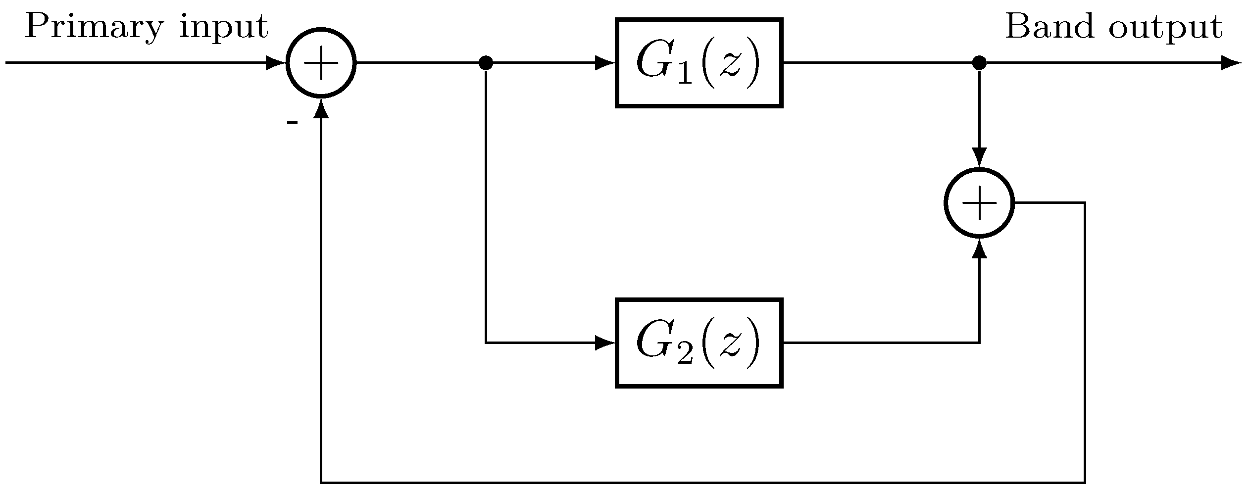
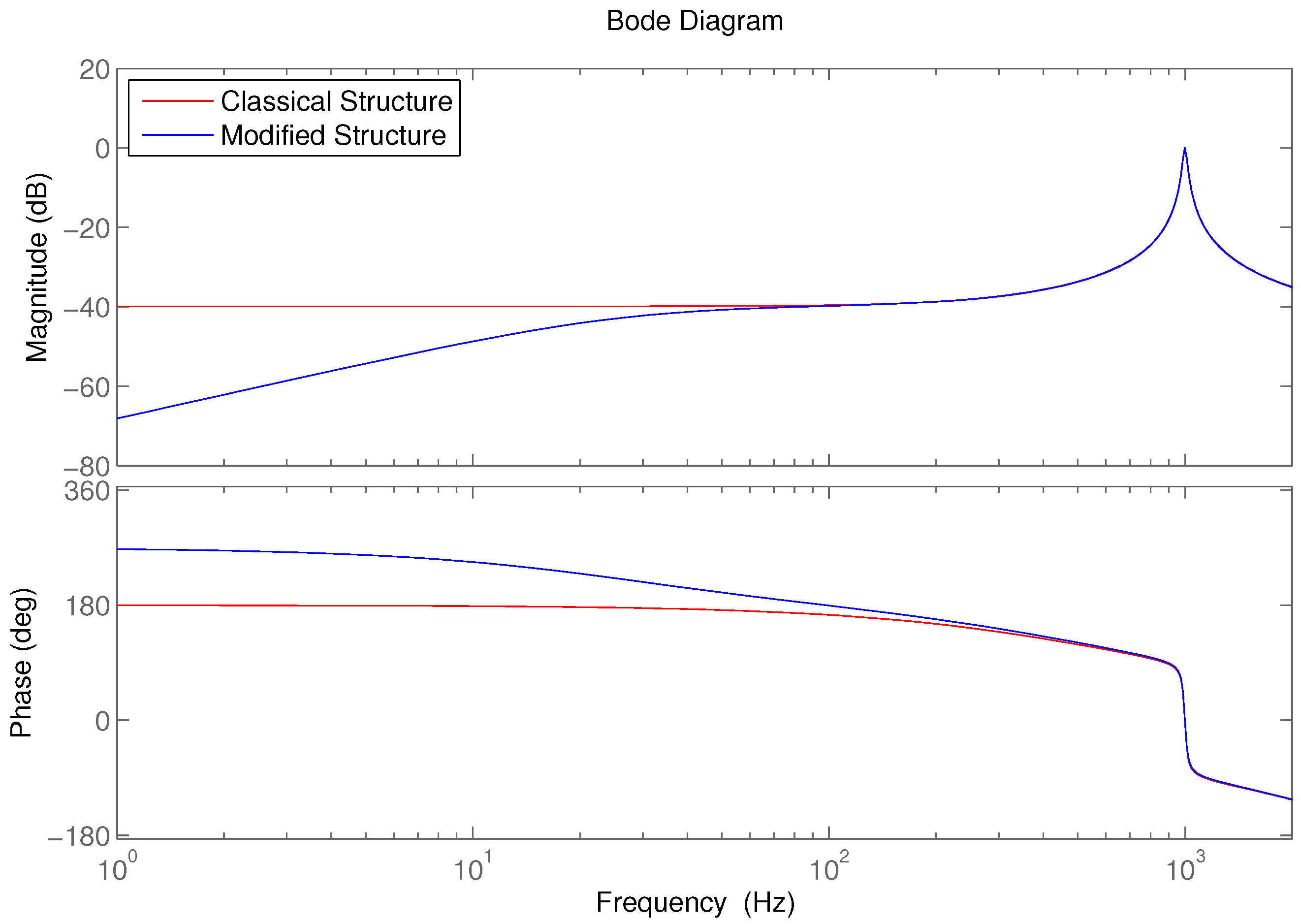
4.2. Structure of the Modified Adaptive Filter

The structure of the modified adaptive filter is shown in Figure 11. Based on the single artificial neuron, the addition of the constant reference input and the weight $w_{3,k}$ bring in a low-pass channel for the adaptive filter. From the perspective of the Fourier series shown as:

$$f\left(x\right)=a_0+a_{1}cos\left(x\right)+b_{1}sin\left(x\right)+\cdots ,$$

(26)

the calculation of $w_{1,k}$, $w_{2,k}$ and $w_{3,k}$ using the adaptive algorithm can be regarded as the seeking process of the Fourier series of the primary input signal.

The LMS algorithm is adopted to update the weights. The detailed iterative process is shown as:

$$\begin{array}{c}{x}_{1,k}=Ccos\left(k{\omega }_0+\varphi \right)\hfill \\ x_{2,k}=Csin\left(k{\omega }_0+\varphi \right)\hfill \\ x_{3,k}=1\hfill \end{array}$$

(27)

$$\begin{array}{c}{w}_{1,k+1}=w_{1,k}+2\mu {\epsilon }_k{x}_{1,k}\hfill \\ w_{2,k+1}=w_{2,k}+2\mu {\epsilon }_k{x}_{2,k}\hfill \\ w_{3,k+1}=w_{3,k}+2\mu {\epsilon }_k{x}_{3,k}\hfill \end{array}$$

(28)

$$y_k=x_{1,k}{w}_{1,k}+x_{2,k}{w}_{2,k}.$$

(29)

The linear transfer function for the adaptive filter from the primary input to the system output can be described as Figure 12, where $G_1\left(z\right)$ is expressed as (22) and $G_2\left(z\right)$ as:

$$G_2\left(z\right)=\frac{2\mu }{z-1}.$$

(30)

The closed-loop transfer function $H^{\prime }\left(z\right)$, from the primary input to the band output, can be expressed as:

$$H^{\prime }\left(z\right)=\frac{G_1}{1+G_1+G_2}.$$

(31)

When $f_0=1000\mathrm{Hz}$ and ${\omega }_0=\pi /4$, the poles’ and zeros’ locations of the transfer function $H^{\prime }\left(z\right)$ are shown in Figure 13. Compared with Figure 9, the original poles’ and zeros’ locations remain almost the same. The difference is the addition of a zero at $(1,0)$ along with a pole in the unit circle meanwhile close to $(1,0)$, as shown in Figure 13. The additional zero and pole, which are close to each other, have little influence on the high frequency property of the proposed filter. Therefore, the conclusion drawn in Section 4.1 about the bandwidth remains valid. The main difference is concentrated in the low frequency characteristic. Due to the addition of the zero at $(1,0)$, the attenuation of the low frequency signal, as shown in Figure 14, is greatly increased compared with the conventional adaptive filter. Meanwhile, the advantage of the adjustable bandwidth is well retained. In brief, the proposed adaptive filter improves the low frequency property with small additional calculation cost. Considering the demand of the sensorless algorithm proposed in Section 3.2 for the BPF, the proposed adaptive filter is fully qualified.

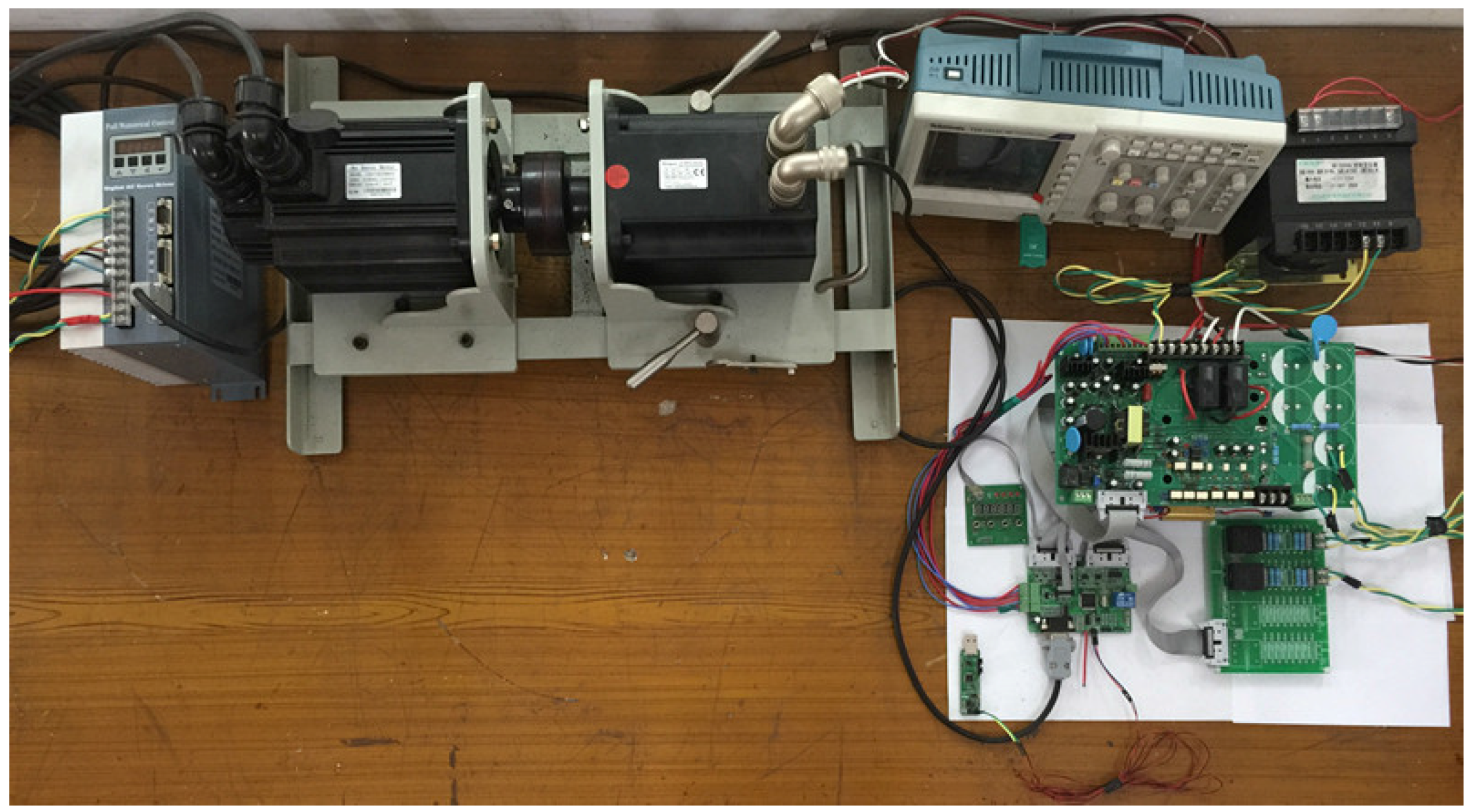
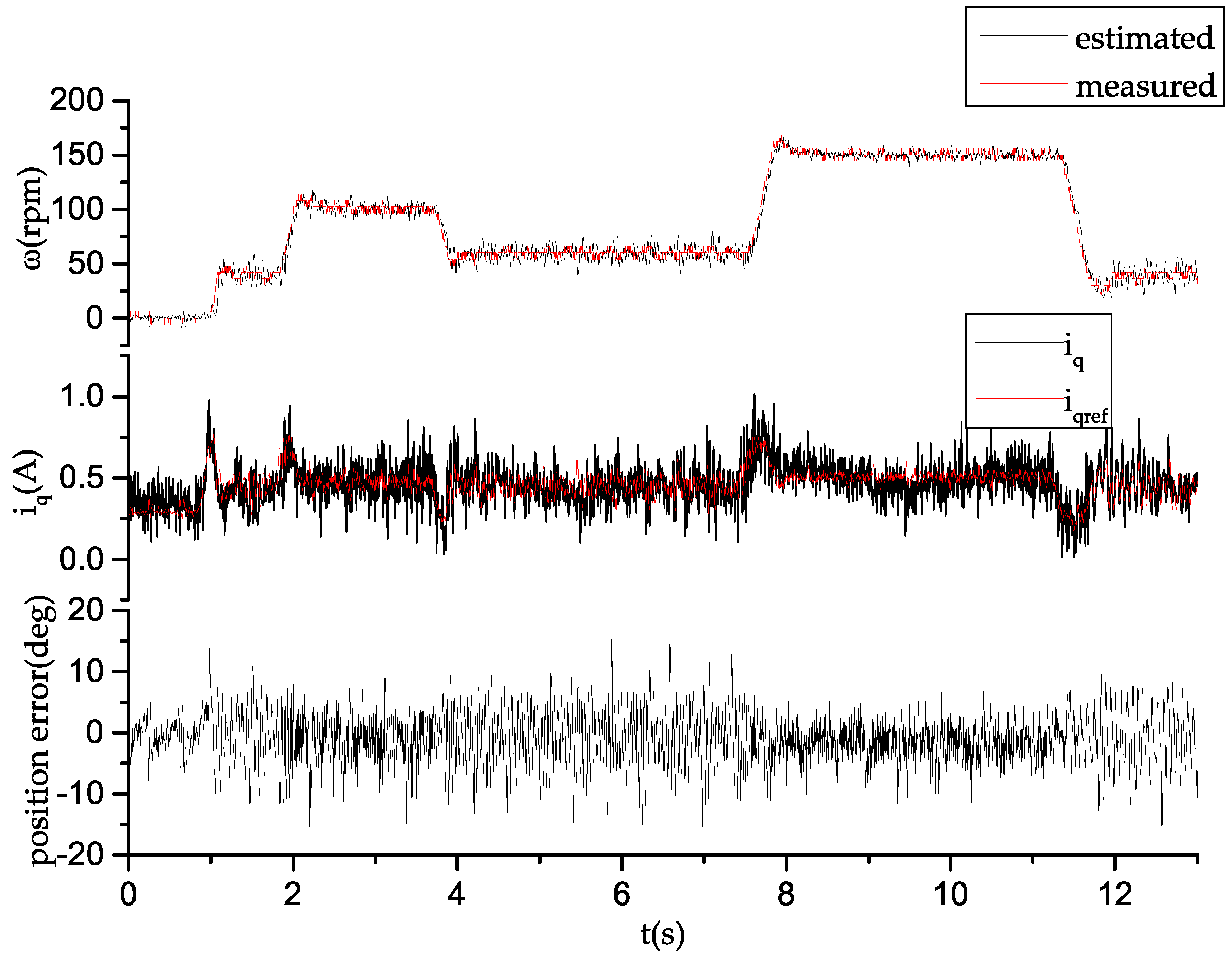
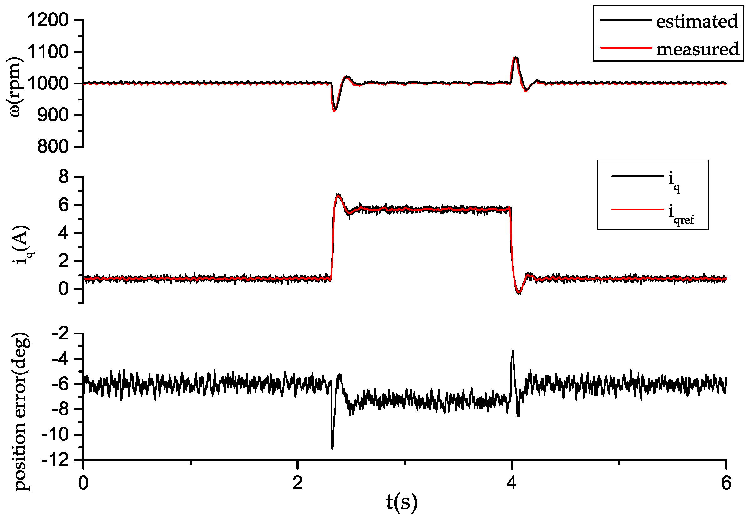
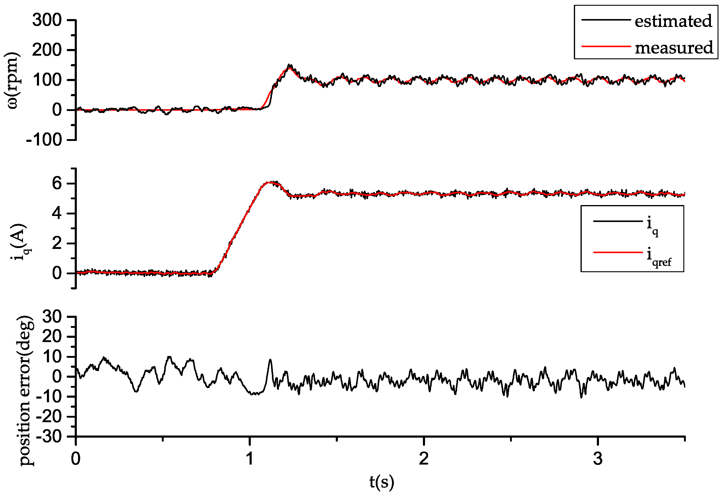
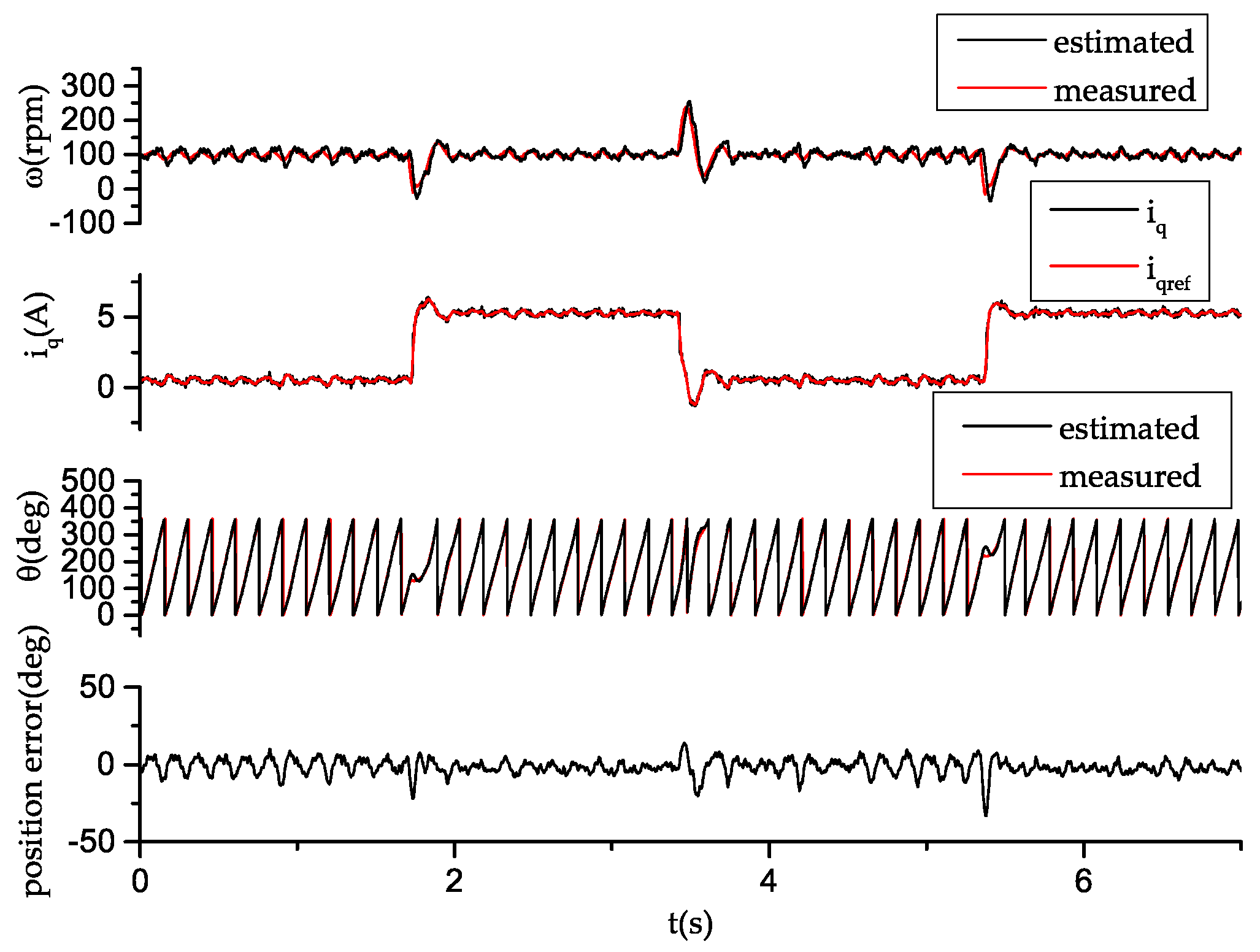
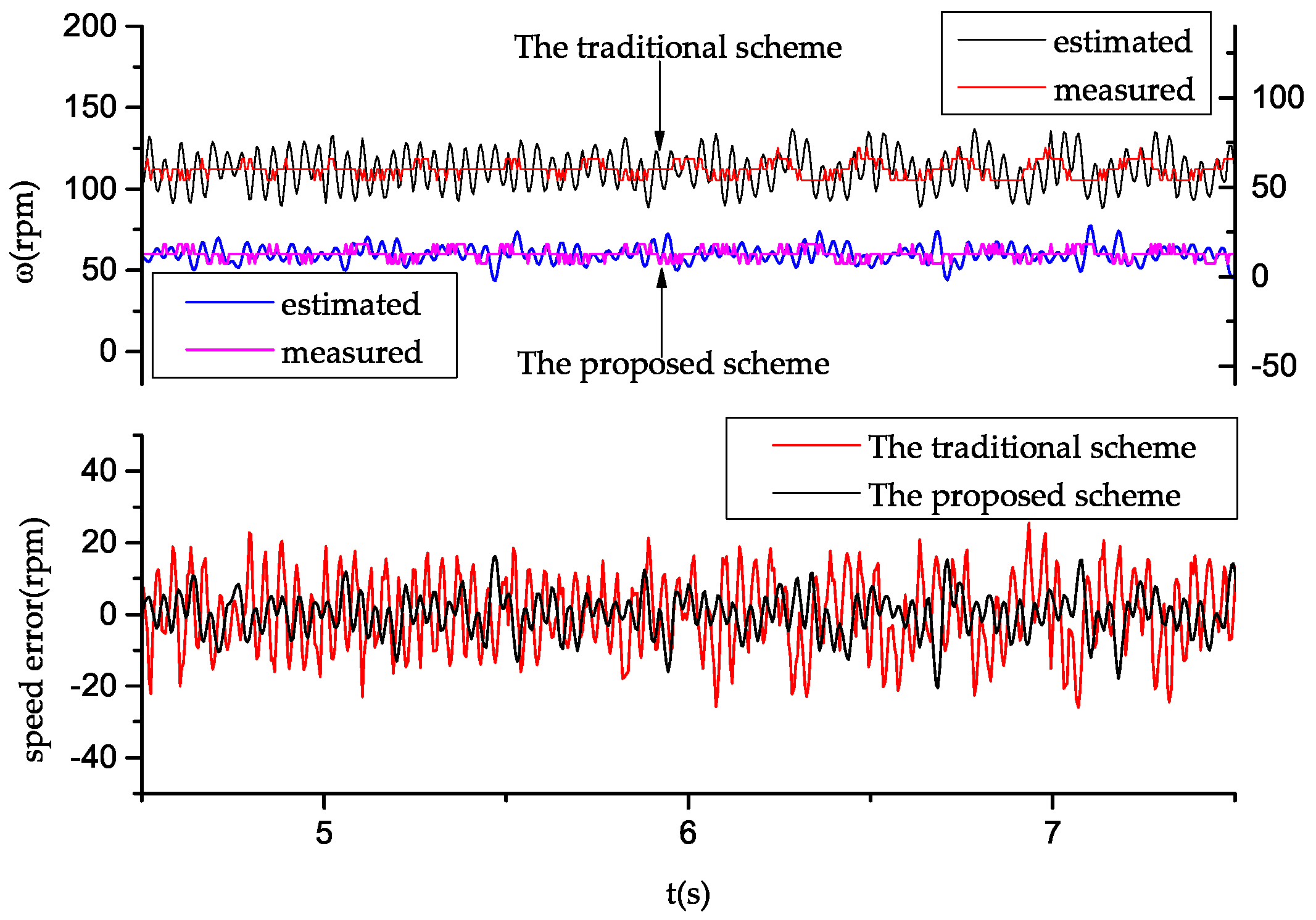
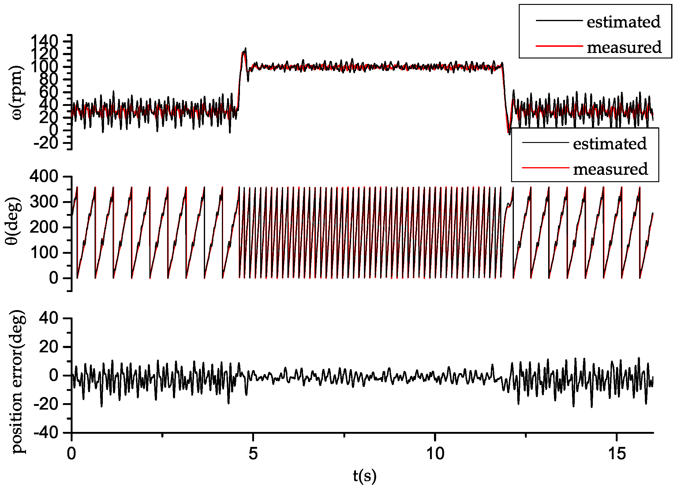
5. Experimental Results

To verify the effectiveness of the proposed sensorless control strategy, the experimental setup is constructed as illustrated in Figure 15. The test IPMSM is fed by a voltage-source inverter using a 10-kHz switching frequency and a 310-V bus voltage. The motor parameters are shown in

Table 1. Motor parameters.

Rating and Parameters	Value	Unit
Rated speed	1500	rpm
Rated torque	7.5	Nm
Number of pole pairs	4	P
Stator resistance	0.49	Ω
d-axis inductance	5.81	mH
q-axis inductance	8.65	mH
rotor flux	0.14	Wb

. The control algorithms are implemented on the STM32F407 floating-point MCU (STMicroelectronics, Geneva, Switzerland), which is based on the ARM Cortex-M4 core (ARM, Cambridge, UK). The phase currents $i_a$ and $i_b$ are sensed by closed-loop hall current sensors. The sample is synchronized to the modulation, which is set at 10 kHz. An photoelectric encoder of 2500 ppr is added only for monitoring the actual rotor speed and position. Another IPMSM controlled by a servo driver is mechanically coupled with the IPMSM to provide the controllable load torque. The frequency of high frequency (HF) signal is chosen as 1 kHz, and its amplitude is selected at 50 V to guarantee the signal-to-noise ratio of the HF current. The deadtime is set as 3 $\mathsf{\mu }$s, and the deadtime compensation strategy is adopted to reduce the position estimation error caused by deadtime effect [26].

The block diagram of the proposed sensorless control strategy is shown in Figure 5b. The improved adaptive filter with center frequency set at 1 kHz is adopted to extract the HF current. The only parameter that needs designing in the PLL-type estimator is ρ, which is set as $2\pi 35$ rad/s considering both static and dynamic performance. The bandwidths of the current and the speed controllers are set around 400 Hz and 40 Hz, respectively. As for the adaptive filter, the LMS algorithm is adopted to update the weights, and the convergence parameter μ is set as 0.3. Compared to the conventional approach shown in Figure 5a, no LPF is needed, and the parameter K equals one, which is independent of the motor parameter.

As for the IPMSM, the initial rotor position is indispensable before the motor starts. In this paper, the initial rotor position is obtained using the proposed HF injection method combined with the dual-pulse polarity detection method [27], which is not described in detail in this paper. Figure 16 shows the experimental results of the start of the process from zero to 100 rpm with a load torque of 4 N·m. It is clear that the estimated speed tracks the actual speed closely during the whole starting process. The maximum position estimation error, which is defined as $\tilde{\theta }=\theta -\widehat{\theta }$, is within ${10}^{\circ }$. The high estimation accuracy ensures the coordinate transform when vector control is conducted. Therefore, the current in the rotor coordinates, $i_q$ for example, tracks the current reference closely, as shown in Figure 16.

Figure 17 shows the experimental results of speed reference steps with no load torque. After the process of initial rotor position detection, the motor starts at 1.2 s from zero to 40 rpm with no load torque. Then, the speed reference is successively set at 100 rpm, 60 rpm, 150 rpm and 40 rpm with the purpose of verifying the dynamic performance of the proposed sensorless control scheme in the low speed region. As shown in Figure 17, the estimated speed tracks the actual speed closely during both the dynamic and steady process. The position estimation error is within ${10}^{\circ }$ during the whole speed regulation process. From Figure 16 and Figure 17, it can be noticed that speed fluctuation exists in both the with and without load torque conditions. In the actual servo system, even if the normal vector control scheme with the encoder is adopted, the speed fluctuation still exists in the low speed region due to the same power of the two machines (braking machine and motor). The speed estimation can be seen as a process of tracking a fluctuant speed reference. Therefore, the parameter ρ ($2\pi 35$ rad/s in this paper) must be selected properly to ensure the bandwidth of the PLL-type estimator.

Figure 18 shows the experimental results of sensorless operation with step load disturbance. From t = 0 s, the test motor operates at 100 rpm with no load. At t = 1.7 s, a load torque of 4 N·m is applied. At t = 3.4 s, the load torque is unloaded. The waveforms of actual and estimated speed are shown in the first plot of Figure 18. The step load disturbances yield large speed transients, and the position error reaches nearly ${25}^{\circ }$ at that moment. During the recovery time, large speed and position estimation errors decrease rapidly. The speed and position estimation can keep up with the drastic changes in the dynamic process and ensure that the normal vector control is implemented smoothly. The position error in the steady operation is controlled within ${10}^{\circ }$.

Figure 5 shows the normal demodulation process of extracting $\tilde{\theta }$-related information and the particular process adopted in this paper to extract ${\widehat{\theta }}_i$-related information. Figure 19 shows the speed waveforms at 60 rpm with the purpose of comparing the steady performance of the two methods. In the contrast experiment, the two schemes share the same control parameters of the current loop, speed loop and speed estimator. For clarity, the speed waveforms are drawn in one plot sharing the same time axis. The upper set of waveforms is the actual and estimated speed waveforms using the normal demodulation process. The speed estimation errors of the two schemes are shown in the lower plot of Figure 19. It is obvious that the waveform of the proposed scheme is less fluctuant. Therefore, the sensorless control scheme proposed in this paper provides better steady state performance than the normal method.

Figure 20 shows the estimation performance with the speed reference as low as 30 rpm. The estimated position can track the real position closely during steady operation and the speed regulation period. The estimated position is shown in the second plot. The position error is within ${15}^{\circ }$ during the whole regulation period. In order to further validate the estimation range and the dynamic performance of the proposed scheme, the speed reference is set at 1000 rpm, as shown in Figure 21. The load of 4 N·m is applied at t = 2.2 s and unloaded 1.8 s later. At the moment that load disturbances occur, large speed transients arise. The proposed speed estimator can keep up with the rapid change of motor speed. The position estimation error is within ${10}^{\circ }$ after the recovery time. In fact, the fundamental excitation methods based on estimating the back EMF are more suitable choices in the medium to high speed region. Even so, the experiment results shown in Figure 21 verify the excellent dynamic performance of the proposed sensorless control scheme. The performance improvement is mainly thanks to the particular structure of obtaining the ${\widehat{\theta }}_i$-related information as shown in Equation (18) and Figure 5b, where the demodulation process in the normal sensorless control scheme is not needed.

6. Conclusions

This paper has presented an improved position estimation scheme. The position estimation error, used as the input of the PLL-type estimator, is extracted directly from the HF current rather than from the demodulation process. The only parameter that needs designing is ρ, which has a direct relation with the static and dynamic performance of the estimator. Therefore, the proposed estimation scheme simplifies the parameter design. Considering the high requirement of the HF current quality, the conventional structure of the adaptive filter is improved by adding a DC channel. The improved adaptive filter provides better attenuation of the low frequency signal, which helps extract the HF current from the DC component. Meanwhile, the advantage of adjustable bandwidth is well retained. According to the experimental results, the proposed sensorless control algorithm realizes the start-up and speed regulation process. Compared with the conventional control scheme, the improved estimation algorithm provides better static performance. The input of the PLL-type estimator does not need to be low-pass filtered, which enables better dynamic performance. The improved adaptive filter ensures enough bandwidth and reduces the estimation error caused by the DC component. The process of the sensorless algorithm, including the estimator technique and the properties of the adaptive filter, has been analyzed in detail. The experimental results verify the feasibility and effectiveness of the proposed sensorless control scheme of IPMSM.

References

1. Holtz, J. Sensorless control of induction motor drives. Proc. IEEE 2002, 90, 1359–1394. [Google Scholar] [CrossRef]
2. Wu, R.; Slemon, G.R. A permanent magnet motor drive without a shaft sensor. IEEE Trans. Ind. Appl. 1991, 27, 1005–1011. [Google Scholar] [CrossRef]
3. Sepe, R.B.; Lang, J.H. Real-Time Observer-Based (Adaptive) Control of a Permanent-Magnet Synchronous Motor without Mechanical Sensors. IEEE Trans. Ind. Appl. 1992, 28, 1345–1352. [Google Scholar] [CrossRef]
4. Jansen, P.L.; Lorenz, R.D. Transducerless Position and Velocity Estimation in Induction and Salient AC Machines. IEEE Trans. Ind. Appl. 1995, 31, 240–247. [Google Scholar] [CrossRef]
5. Shinnaka, S. New “D-state-observer”-based vector control for sensorless drive of permanent-magnet synchronous motors. IEEE Trans. Ind. Appl. 2005, 41, 825–833. [Google Scholar] [CrossRef]
6. Piippo, A.; Hinkkanen, M.; Luomi, J. Analysis of an adaptive observer for sensorless control of interior permanent magnet synchronous motors. IEEE Trans. Ind. Electron. 2008, 55, 570–576. [Google Scholar] [CrossRef]
7. Alahakoon, S.; Fernando, T.; Trinh, H.; Sreeram, V. Unknown input sliding mode functional observers with application to sensorless control of permanent magnet synchronous machines. J. Frankl. Inst. 2013, 350, 107–128. [Google Scholar] [CrossRef]
8. Kim, H.; Son, J.; Lee, J. A high-speed sliding-mode observer for the sensorless speed control of a PMSM. IEEE Trans. Ind. Electron. 2011, 58, 4069–4077. [Google Scholar]
9. Bolognani, S.; Tubiana, L.; Zigliotto, M. Extended Kalman filter tuning in sensorless PMSM drives. IEEE Trans. Ind. Appl. 2003, 39, 1741–1747. [Google Scholar] [CrossRef]
10. Quang, N.K.; Hieu, N.T.; Ha, Q.P. FPGA-based sensorless PMSM speed control using reduced-order extended kalman filters. IEEE Trans. Ind. Electron. 2014, 61, 6574–6582. [Google Scholar] [CrossRef]
11. Hinkkanen, M.; Tuovinen, T.; Harnefors, L.; Luomi, J. A combined position and stator-resistance observer for salient PMSM drives: Design and stability analysis. IEEE Trans. Power Electron. 2012, 27, 601–609. [Google Scholar] [CrossRef]
12. Holtz, J. Acquisition of position error and magnet polarity for sensorless control of PM synchronous machines. IEEE Trans. Ind. Appl. 2008, 44, 1172–1180. [Google Scholar] [CrossRef]
13. DeKock, H.W.; Kamper, M.J.; Kennel, R.M. Anisotropy Comparison of Reluctance and PM Synchronous Machines for Position Sensorless Control Using HF Carrier Injection. IEEE Trans. Power Electron. 2009, 24, 1905–1913. [Google Scholar] [CrossRef]
14. Jang, J.H.; Sul, S.K.; Ha, J.I.; Ide, K.; Sawamura, M. Sensorless Drive of Surface-Mounted Permanent-Magnet Motor by High-Frequency Signal Injection Based on Magnetic Saliency. IEEE Trans. Ind. Appl. 2003, 39, 1031–1039. [Google Scholar] [CrossRef]
15. Corley, M.; Lorenz, R. Rotor position and velocity estimation for a salient-pole permanent magnet synchronous machine at standstill and high speeds. IEEE Trans. Ind. Appl. 1998, 34, 784–789. [Google Scholar] [CrossRef]
16. Briz, F.; Degner, M.W.; Garcia, P.; Lorenz, R.D. Comparison of saliency-based sensorless control techniques for AC machines. IEEE Trans. Ind. Appl. 2004, 40, 1107–1115. [Google Scholar] [CrossRef]
17. Liu, J.M.; Zhu, Z.Q. Sensorless Control Strategy by Square-Waveform High-Frequency Pulsating Signal Injection Into Stationary Reference Frame. IEEE J. Emerg. Sel. Top. Power Electron. 2014, 2, 171–180. [Google Scholar] [CrossRef]
18. Krishnan, R. Permanent Magnet Synchronous and Brushless DC Motor Drives; CRC Press: New York, NY, USA, 2010; pp. 423–451. [Google Scholar]
19. Widrow, B.; Stearns, S. Adaptive Signal Processing; Prentice-Hall: Englewood Cliffs, NJ, USA, 1985; pp. 302–361. [Google Scholar]
20. Accetta, A.; Cirrincione, M.; Pucci, M.; Vitale, G. Sensorless control of PMSM fractional horsepower drives by signal injection and neural adaptive-band filtering. IEEE Trans. Ind. Electron. 2012, 59, 1355–1366. [Google Scholar] [CrossRef]
21. Wang, G.; Li, T.; Zhang, G.; Gui, X.; Xu, D. Position estimation error reduction using recursive-least-square adaptive filter for model-based sensorless interior permanent-magnet synchronous motor drives. IEEE Trans. Ind. Electron. 2014, 61, 5115–5125. [Google Scholar] [CrossRef]
22. Stensby, J. Phase-Locked Loops: Theory and Applications; CRC Press: New York, NY, USA, 1997; pp. 211–252. [Google Scholar]
23. Harnefors, L.; Nee, H.P. A general algorithm for speed and position estimation of AC motors. IEEE Trans. Ind. Electron. 2000, 47, 77–83. [Google Scholar] [CrossRef]
24. Wallmark, O.; Harnefors, L.; Carlson, O. An improved speed and position estimator for salient permanent-magnet synchronous motors. IEEE Trans. Ind. Electron. 2005, 52, 255–262. [Google Scholar] [CrossRef]
25. Piippo, A.; Salomaki, J.; Luomi, J. Signal injection in sensorless PMSM drives equipped with inverter output filter. IEEE Trans. Ind. Appl. 2008, 44, 1614–1620. [Google Scholar] [CrossRef]
26. Wang, G.; Yang, R.; Xu, D. DSP-based control of sensorless IPMSM drives for wide-speed-range operation. IEEE Trans. Ind. Electron. 2013, 60, 720–727. [Google Scholar] [CrossRef]
27. Holtz, J. Initial rotor polarity detection and sensorless control of PM synchronous machines. In Proceedings of the Conference Record of the 2006 IEEE Industry Applications Conference, 41st IAS Annual Meeting, Tampa, FL, USA, 8–12 October 2006.
Figure 1. Relationship between the real coordinates and the estimated coordinates.
Energies 09 01084 g001
Figure 2. Flowchart of the PLL-type estimator.
Energies 09 01084 g002
Figure 3. Block diagram of the proposed sensorless drive.
Energies 09 01084 g003
Figure 4. The space position of the high frequency current vector. (a) The d ^ -axis lags the d-axis; (b) the d-axis lags the d ^ -axis.
Energies 09 01084 g004
Figure 5. Procedure of signal processing. (a) Procedure of signal processing to extract θ ˜ -related information; (b) procedure of signal processing to extract θ ^ i -related information.
Energies 09 01084 g005
Figure 6. The oscillating current vector i c in the estimated coordinates.
Energies 09 01084 g006
Figure 7. Structure of the adaptive filter.
Energies 09 01084 g007
Figure 8. The linear transfer function for the adaptive filter.
Energies 09 01084 g008
Figure 9. Poles’ and zeros’ locations of the transfer function H z .
Energies 09 01084 g009
Figure 10. The magnitude-phase characteristic of H z : C = 1 , μ = 0.01 (red line); C = 1 , μ = 0.001 (blue line).
Energies 09 01084 g010
Figure 11. Structure of the modified adaptive filter.
Energies 09 01084 g011
Figure 12. The linear transfer function for the modified adaptive filter.
Energies 09 01084 g012
Figure 13. Poles’ and zeros’ locations of the transfer function H z .
Energies 09 01084 g013
Figure 14. The magnitude-phase characteristic of H z and H z when C = 1 , μ = 0.001 : classical structure H z (red line); modified structure H z (blue line).
Energies 09 01084 g014
Figure 15. Photograph of the experimental setup.
Energies 09 01084 g015
Figure 16. Experimental results of the start process, including the waveforms of actual and estimated speed, current i q and i q reference and position estimation error.
Energies 09 01084 g016
Figure 17. Experimental results of speed reference steps with no load torque, including the waveforms of actual and estimated speed, current i q and i q reference and position estimation error.
Energies 09 01084 g017
Figure 18. Experimental results of sensorless operation with step load disturbance.
Energies 09 01084 g018
Figure 19. The steady performance comparison of two sensorless control schemes.
Energies 09 01084 g019
Figure 20. The estimation performance of speed reference steps: 30 rpm–100 rpm–30 rpm.
Energies 09 01084 g020
Figure 21. The dynamic performance of the proposed scheme with the speed reference set at 1000 rpm.
Energies 09 01084 g021