Design of an Energy Efficient Future Base Station with Large-Scale Antenna System


1
School of Intelligent Mechatronic Engineering, Sejong University, Seoul 05006, Korea
2
Department of Electronic Engineering, Kwangwoon University, Seoul 01897, Korea
*
Author to whom correspondence should be addressed.
Energies 2016, 9(12), 1083; https://doi.org/10.3390/en9121083
Submission received: 6 October 2016
/
Accepted: 12 December 2016
/
Published: 17 December 2016
Abstract
:Due to the continuous increase in data demanded by end-users, an energy-efficient base station (BS) is a vital topic of interest that would not only result in a substantial economic impact on service providers, but would also reduce the carbon footprint of operating a network. In this regard, we propose the structure and systematic operation of a BS with a large-scale (LS) antenna system that can increase the energy efficiency (EE) of cellular systems. The proposed BS structure includes various power-related units, such as a central management apparatus, power controller, EE calculator, radio site-dependent parameter space (RSD-PS) and determiner. With the information provided from each unit, the decision unit determines how to adjust each component of the BS in order to maximize the EE. Extensive simulations show that the proposed BS improves the EE performance by about relative to the reference BS.

1. Introduction
Communication technologies that can increase channel capacity, as well as energy efficiency (EE) would be a key factor for future wireless systems. An increase in EE is very important because the continuous increase in data demanded by end-users results in a high cost both from an environmental and technological perspective. It is well known that base stations (BS) consume around 60%–80% of power consumption in cellular networks [1,2,3]. Thus, reducing the power consumption of a BS is quite important to reduce the operational costs, as well as the carbon footprint. For this reason, researchers have actively investigated this problem [1,2,4,5,6,7,8,9,10,11,12,13,14,15]. Most work has concentrated on implementing the BS on/off technique, which means that the BS is turned off when there is no nearby traffic [1,2,9,10,12,14], as well as on conducting theoretical high-level analyses and optimizations to reduce the BS power consumption [7,8,11,13]. However, the BS on/off technique is only beneficial for an empty network, which rarely happens in actual networks. Furthermore, there could be many real implementation obstacles for theoretical, high-level optimization techniques.
In this paper, rather than presenting a BS on/off mechanism or solving the theoretical optimization problem, we focus on more practical implementation aspects to improve the EE of cellular systems. We propose a future energy-efficient BS structure and its related operation using a realistic power model for real implementation. Due to the limited spectrum resources, it is also inevitable for the number of transmitter (TX) antennas in the BS to continuously increase [11]. Thus, we assume that a future BS has a large number of TX antennas, that is a large-scale (LS) antenna system or LS multiple-input multiple-output (MIMO) [16,17,18]. Actually, in the case of a BS with LS-MIMO, the resource allocation problems are easier to solve if the channel properties provided by LS-MIMO systems are exploited smartly [19,20].
The proposed energy-efficient BS consists of five main components: a central management apparatus, power controller, EE calculator, radio site-dependent parameter space (RSD-PS) and determiner. The central management apparatus manages the appropriate power consumption of each BS located in a pre-defined range. The power controller controls the power control of each related device. The EE calculator, which operates based on the power consumption and data rate estimator, provides the power control metric. The RSD-PS accumulates information and supports the increase in EE according to past operation information. The determiner for each decision unit decides the operation points of the power-related devices for a pre-defined time duration. Each component can also be divided into several sub-components. With these components, we show how to systematically increase the EE of the proposed future BS. The BS could also be used as a hub for a LS sensor system for a smart city or such.
In what follows, we introduce the system model in Section 2. In Section 3, we present the proposed BS structure and the method used to systematically increase the EE of the BS. In Section 4, we present numerical results based on a reference future BS model, showing the effectiveness of the proposed structure and method. Finally, the conclusions are drawn in Section 5.
2. System Model
This section describes the power consumption model and the LS-MIMO model, which are the core models used in the performance analysis of the proposed BS.
2.1. Power Consumption Model
Modeling the BS power consumption is an important problem to measure the EE. A typical BS is composed of many power consumption components, including a supply, cooling, baseband (BB), radio frequency (RF), power amplifier (PA), loss factors for DC-DC, feeding cable, and so on [5]. Some studies have roughly divided this into static power and dynamic power [21]. It is difficult to estimate how technology would evolve, and designing an exact model is beyond the scope of this paper. However, a realistic model could be helpful in analyzing the proposed methods. In this paper, we define the total power for a tractable power consumption model that includes some of the important BS power consumption components. We define as:
where is the PA power consumption and is the circuit power consumption except for the PA power consumption, including the BB power consumption, , and RF front-end power consumption, . In this model, since maximum radiation power is limited regardless of the number of TX antennas , we should keep in mind that can be reduced with the help of a beamforming effect, while increases as increases. We describe below each of the power consumption components in further detail.
2.1.1. Power Amplifier
The PA is one of the most power-hungry devices in the current BS. Current cellular standards, i.e., 3GPP-LTE-A, IEEE 802.16 (e/m), use orthogonal frequency division multiplexing (OFDM) for downlink transmission. The OFDM has a very high peak-to-average power ratio (PAPR), and this significantly reduces the PA efficiency [22]. If we assume a 10-MHz BW with a 1024 IFFTsize, with less than a distortion probability or complementary cumulative distribution function (CCDF), PAPR is known to be higher than 11 dB. Based on this, we choose an input-back-off (IBO) = 11 dB [22]. We also simply assume the use of the maximum efficiency of the Class-B amplifier (). Then, the PA efficiency, η, can be represented as [23,24]:
where the p is the . Depending on the parameters that we mentioned, the PA efficiency can be . However, various advanced technologies can be applied to obtain an increase by more than that, and thus, we reasonably choose . The simple relation between the transmission power and can be represented as:
It is possible for the TX power to be reduced if we increase the , due to the channel gain increment. Note that we assume the system does not adopt any predistortion and/or PAPR reduction techniques.
2.1.2. Circuits Power Consumption
The circuit power consumption can also be divided as follows:
Each parameter is a function of bandwidth, B, and we use MHz. can also be divided as:
where is the digital-to-analog converter (DAC) power consumption, is the mixer power consumption and is the TX filter power consumption [25].
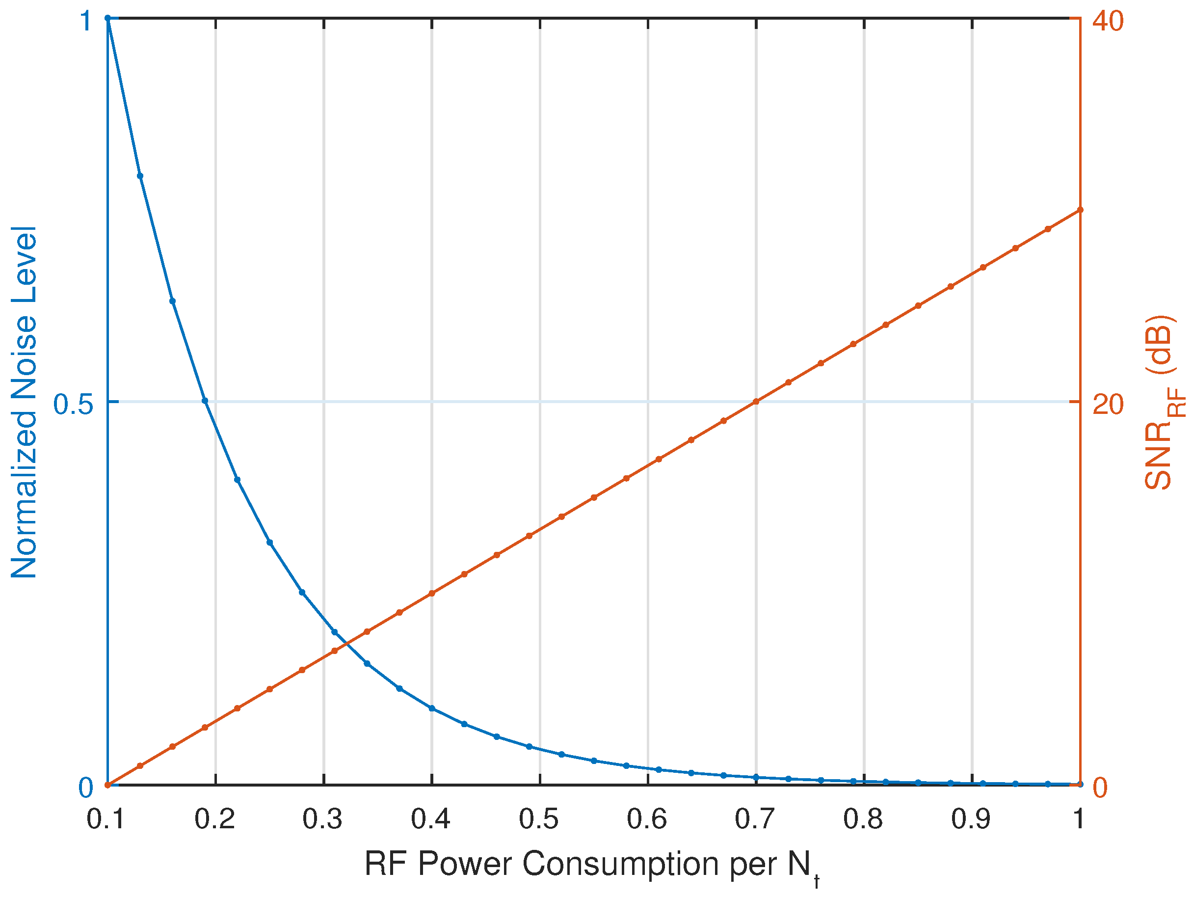
In this paper, we assume that we can adjust the RF power consumption. It would then be obvious for fine DAC/filtering to be difficult if we reduce the RF power consumption. Based on this assumption, we propose the RF power consumption model shown in Figure 1. This model indicates that the performance of the RF front-end circuits depends on the power consumption of those. For example, assuming we can adjust the RF power consumption from 0.1 to 1 W, when the RF power consumption = 0.1 W, the noise from coarse processing is too high, and , the signal to RF noise ratio due to coarse processing, is 0 dB, i.e., the noise level and signal level are the same. Meanwhile, is 20 dB, when RF power consumption = 0.7 W, and a relative level of fine RF processing is possible. Regarding the BB power consumption, , we already mentioned that we assume a future BS to have LS-MIMO capability. With that in mind, H.Yang and T. Marzetta presented an LS-MIMO BB computation model, , which is denoted as follows [26,27,28]:
where is the length in the samples of the uplink pilot sequences, which are used to acquire channel state information (CSI), and a description of each parameter is shown in Table 1. We took the parameters from [29] and from a current LTE system [30]. The first part of Equation (6) is to operate the FFT/IFFT operation; the second part is to implement precoding/decoding; the third part is to correlate the pilot signals with pilot sequences; and the last part is to have the additional pseudo inverse for zero-forcing (ZF).
The relationship between and can be represented as:
where ϱ is the very-large-scale integration (VLSI) processing efficiency.
We assume , a short guard interval (GI) and fast pilot correlation. Three pilot symbols are dedicated to one slot for the channel estimation [29]. Note that this model does not include a channel coding part, and the last part of Equation (6) becomes zero, when we use matched filtering (MF) precoding.
2.2. Large-Scale Multiple-Input Multiple-Output Model
In this subsection, we summarize the LS-MIMO model since the LS-MIMO would be a very important characteristic of a future BS. An LS-MIMO is an antenna system with a large number of TX antennas. It was first introduced by Marzetta [29], and after that, much research has been carried out [19,20,28]. Due to its desirable improvements in throughput (TP) and EE, it has already been discussed by the important standardization body, i.e., the the 3rd Generation Partnership Project (3GPP), as one of the core technologies for 5 G. In 3GPP, the LS-MIMO is usually referred to as full-dimension MIMO (FD-MIMO). Therefore, it is unquestionable for the LS-MIMO to be a key technology for future BS.
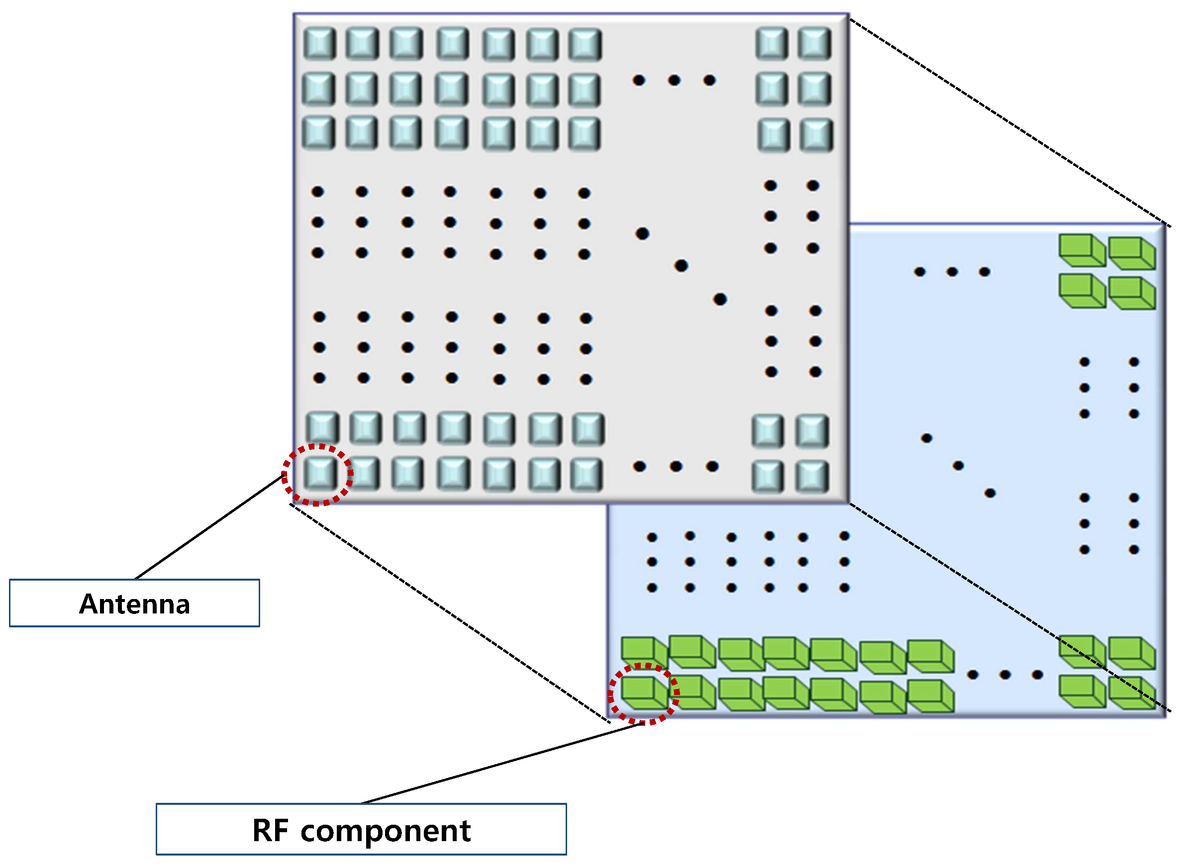
The antenna structure of a BS equipped with LS-MIMO could be of various shapes depending on the implementation. One example of a high-level conceptual figure of an LS-MIMO system is shown in Figure 2.
Each antenna has its own RF component, as shown in Figure 3, and the structure in Figure 2 and Figure 3 can be used to generate a very sharp beam. The designer can choose to put more antennas in the vertical direction or horizontal direction. If we put more antennas in the vertical direction, the resolution of the vertical beam separation is very good, and thus, users who are located on each floor of a building can benefit. If we put more antennas in the horizontal direction, it can provide a horizontal separation effect, and thus, users located in different horizontal angles can benefit.
However, there are some obstacles to realize LS-MIMO. First, the antenna spacing should be at least , which means that it requires a quite large space for installation and use with cellular bands. Even though higher frequency bands could be a good option, the poor channel condition should be overcame. Second, it requires many RF chains, which are very expensive. Good antenna selection algorithms can be very helpful to reduce the number of RF chains [16]. Thus, implementing LS-MIMO with a low complexity and cost is a big research topic.
To introduce the operation of the LS-MIMO system, let us think of a single isolated cell with one BS and Kuser terminals. The BS has TX antennas, and each user terminal has one RX antenna. The received signal vector at the terminals can be represented as follows:
where is the received signal vector for K user terminals, is the total TX power for the downlink, is the channel matrix between BS antennas and K terminals, is the TX signal vector and is the noise (AWGN) vector at the terminals. The element of the channel matrix between the m-th BS antenna and the k-th terminal, can be decomposed as:
where is the zero-mean and unit variance i.i.d. Rayleigh fading channel coefficient and is the path loss component. We only consider the narrowband signal, since the OFDM can successfully change the wideband signal into a narrowband signal. The TX is assumed to have perfect CSI. To show the channel hardening effect with LS-MIMO, it is usually required for K, which means that the number of TX antennas in the BS should be much more than the number of users [16].
2.2.1. Precoding Method
Precoding is an MIMO TX signal processing method that reduces the interference among the users. Since would be very large in a future BS equipped with LS-MIMO, linear precoding is tractable for real systems. ZF and regularized zero-forcing (RZF) are well known as effective linear precoding techniques [31,32]. Furthermore, T. Marzetta suggested an even simpler precoding technique, MF precoding [29]. MF precoding is only effective for LS-MIMO, while ZF/RZF precoding is also useful for traditional MIMO. The relation between the TX signal vector, , and the massage signal vector, , is expressed as follows:
where ζ is the TX power normalization factor and is the precoding matrix.
Then, (8) can be rewritten as:
All three precoding matrices are presented in Table 2.
In the table, superscript “H” denotes the conjugate transpose, is the inverse operator and is the identity matrix. RZF precoding can be the same as ZF and/or minimum mean square error (MMSE) precoding if we choose and/or .
As grows without bounds, the autocorrelation of the channel vectors can be simplified as follows [29]:
Simply, we call (12) an LS-MIMO channel characteristic. If we apply (12) to the MMSE and the ZF, the MMSE and the ZF can be simplified as [16]:
This means that with an excessive number of TX antennas with a limited number of RX antennas, all representative linear precoding techniques show similar performance. ZF is well known to be near optimal in a region with very high SNR. If we consider the complexity of the nonlinear precoding techniques and high effective signal-to-interference plus noise ratio (SINR) of the LS-MIMO systems, linear precoding would show sufficient performance with low complexity.
Now, let us determine the normalization factor ζ. The normalization factor should be determined such that the total transmit power becomes . This means:
where stands for the Frobenius norm.
Since and are independent, and we already choose the average power of the signal constellation in unity, ζ can be represented as [16]:
The ZF and MMSE precoding show a very similar performance, even with a relatively practical number of LS TX antennas (i.e., K). For this reason, we only use MF and ZF as precoding techniques in this paper.
2.2.2. Throughput and Energy Efficiency
The TP and EE are two important metrics that can be used to conduct a performance analysis.
Based on the analysis from previous subsections, the symbol received by the k-th user is given as follows [29]:
where is the channel vector for the i-th user and is the precoding vector for the i-th user. The last term of (16) is inter-user interference (IUI). Then, the effective SINR for user k, , can be represented as follows [4]:
where is the noise power in the given bandwidth B.
If we increase the number of TX antennas or reduce the number of users, it is obvious that we can get better channel gain and/or an effective SINR. However, we should keep in mind that, in the practical number of TX antennas, MF precoding does not remove the IUI completely.
Based on (17), we can define TP as follows:
where is the scaling factor for the pilot overhead and guard interval [29].
EE can be defined as:
We will use (19) as the metric for the performance analysis in the following sections.
3. Energy-Efficient BS Structure and Related Operation
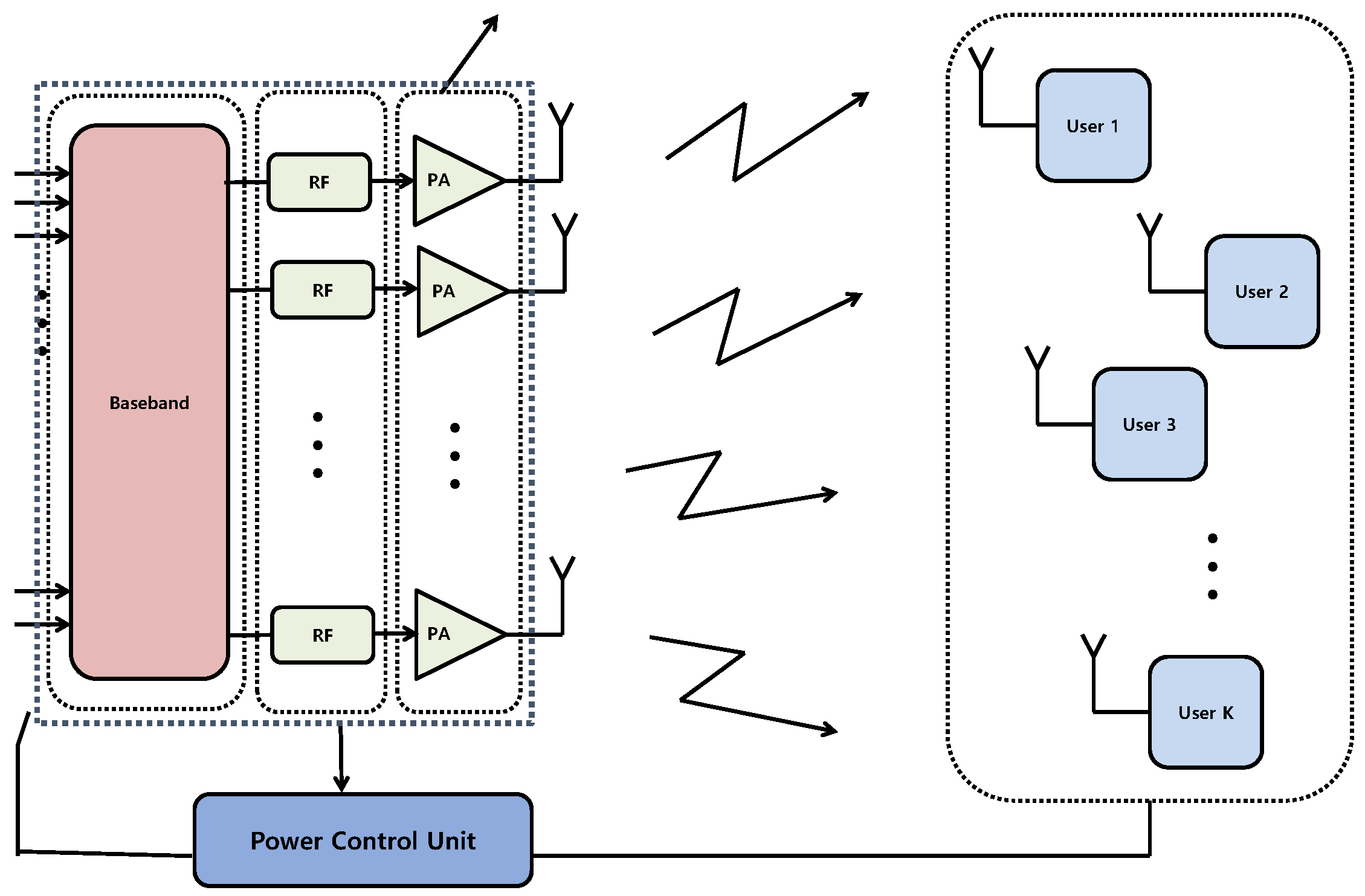
To achieve a high EE for the BS, it is essential to control some of the important TX parameters there. We can divide the main BS power consumption components in PA, RF (except PA) and BB and make out each component to be a power-adjusting component. The PA is the most power-hungry device in the current BS, but this could change depending on the situation of a future BS. Since a future BS could have a large amount of RF chains connected to each antenna, it is also possible for the RF chain to consume more power than the PA. In contrast to the PA, which can reduce the power consumption by using a beamforming effect, there are no distinct sources to reduce the RF chain power consumption. The BB may consume less power when compared to the PA and RF. However, it is better to include it as one of the adjustable parameters to enhance the EE. The three main components can be controlled as shown in Figure 4.
An energy-efficient future BS is quite obviously a feedback system. It mainly receives information of the power consumption from the BS TX unit and information regarding the data rate from the user terminals. As shown in the figure, the power control unit controls each component based on the measured EE parameters. The proposed BS measures the data rate, and if it is not in a satisfactory range, it provides an input to power the adjustable unit to increase the power consumption of some of the components. Then, based on the power adjustment of each component, the data rate estimation unit measures the data rate again and checks if it is in the satisfactory range, and so on. If the power consumption is too high over a pre-defined threshold, then the data rate could also be reduced to obtain satisfactory EE performance.
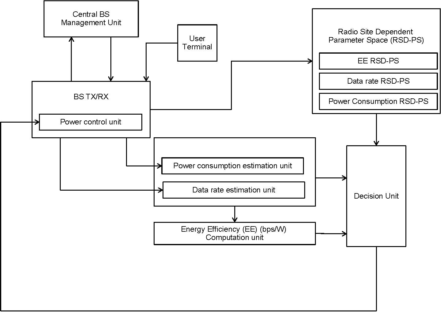
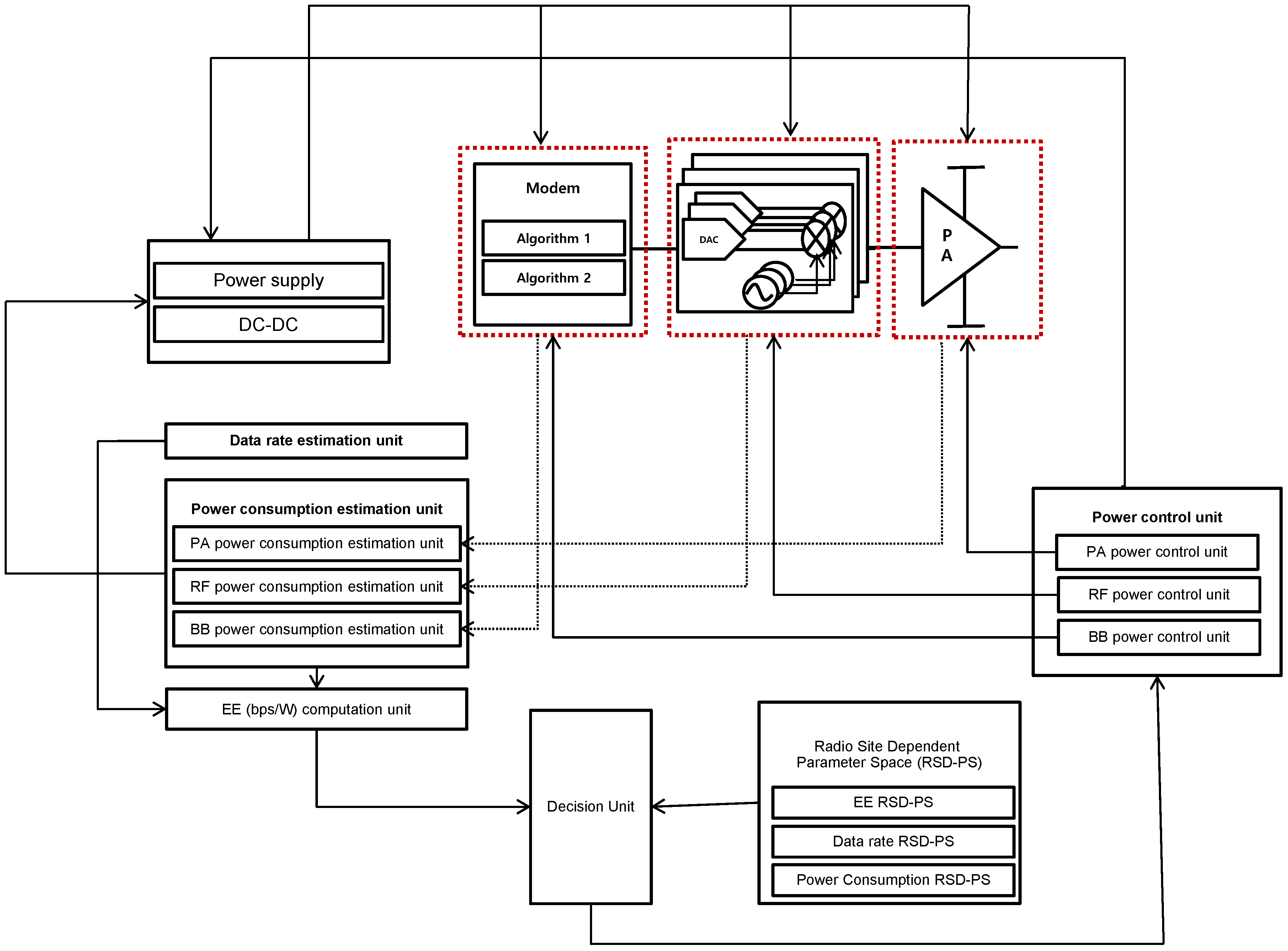
Based on the high-level concept of a future BS, the detailed block diagram of the proposed BS structure is described in Figure 5.
First, let us observe two units, the power consumption estimation unit and the data rate estimation unit, which are tightly connected with the fundamental TX/RXunit of the BS. The BS provides information for the units based on feedback from self-measurement and user terminals, then EE (bps/W) can be derived based on the results. All information (power consumption, data rate, EE) is given to the decision unit, which can then decide each component’s power consumption, i.e., PA, RF and BB. The decision unit provides feedback on the decision to the fundamental TX/RX unit of the BS. Then, the BS performs power control based on the feedback information.
There are three more components in this structure, as shown in the figure. The first one is the central BS management unit. This apparatus can be used for multi-BS power control/optimization. The central BS management unit monitors all nearby BSs and adaptively allocates the allowable maximum power for each BS. Then, each BS only allocates power for each component based on the total allowable power consumption criterion. The second one is the user terminal. In particular, the data rate can be easily measured with a user terminal. Furthermore, it is beneficial for the user terminal to give feedback regarding the current channel condition. The last one is the RSD-SP. The RSD-SP is the apparatus that accumulates the history of optimum BS operation, and supports the decision unit to determine the operating points of BS based on the accumulated history whenever necessary. For example, RSD-PS monitors the BS operation, such as the level of radiation power, the level of the resolution of the RF chain, the level of BB processing based on operating parameters, such as the number of TX antennas, the number of users, system bandwidth, the channel condition, and so on. After having accumulated enough, the RSD-PS can assist to maintain the high EE BS by providing the history of optimum EE operation points based on operation parameters. The BS can get even higher energy savings by skipping the real calculation of operation points for some interval. The system parameters for the operation of an energy-efficient BS is summarized in Table 3.
Note that the performance of the proposed power control scheme critically depends on the threshold of the data rate and power consumption. The threshold is a bandwidth-limited regime and a power-limited regime in Shannon’s channel capacity. Increasing power guarantees increasing the data rate significantly up to the power-limited regime in channel capacity. However, if the system goes to the bandwidth-limited regime in channel capacity, the data rate is no longer increased significantly, even if we increase it with large amounts of the power.
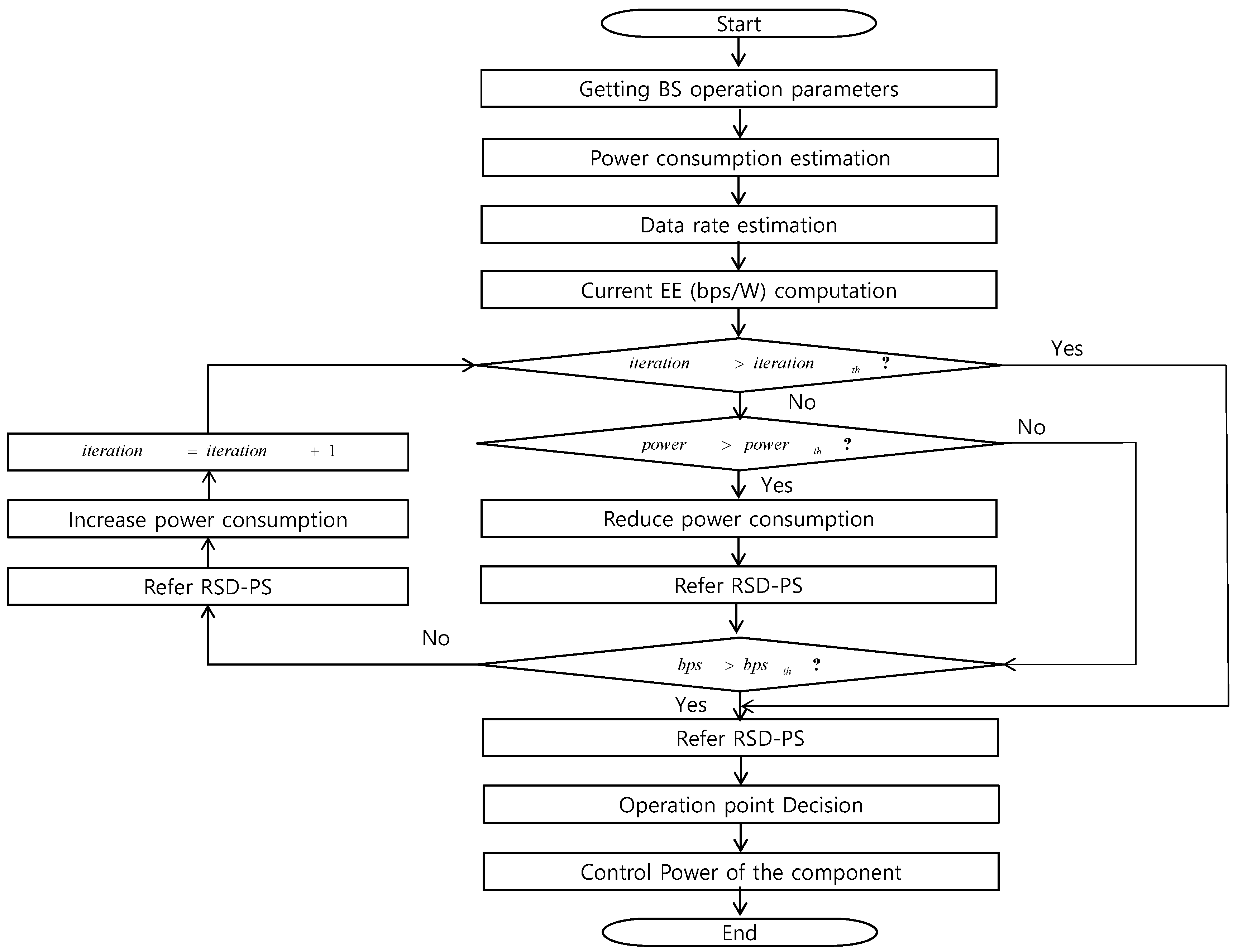
There are various ways to adjust the TP or data rate and EE using the power control, as shown in Table 4. There is a trade-off between the EE and TP. However, if we appropriately allocate power for each component, it could be possible to increase both EE and TP, such as when using big data/machine learning-based RSD-PS. To show the systematic operation of the proposed BS, we provide one example using a flow chart, as shown in Figure 6.
After gathering important parameters from the BS TX parts and user terminals, the proposed BS can derive the EE based on the power consumption estimation and data rate estimation. We set the number of iterations for the parameter adjustment between the data rate and the power consumption to obtain the expected performance, as well as to reduce the complexity. If the pre-defined number of iterations is smaller than the current number of iterations, then the iteration stops, and the BS finds the operation point based on the information of the current parameters and the RSD-PS. If not, the proposed BS estimates whether the current power consumption is larger than the threshold for the power consumption. If the current power consumption is larger than the threshold, the proposed BS reduces the power consumption in appropriate ways by using the RSD-PS. Then, the proposed BS checks the TP. If the TP is within the satisfactory range, with the help of RSD-PS, the proposed BS determines the operating point. If the TP is not in a satisfactory range, the proposed BS goes to the loop and increases the power consumption to obtain a better TP, and so on.
A proper power control algorithm should be included to reduce inter-cell interference. After achieving an operating point, the BS could operate with the operating point for a while. After that, the process could be performed again because the optimum point can change anytime in a dynamic wireless environment. Note that the operating procedure can be determined in various ways based on the proposed BS structure.
4. Numerical Results
In this section, we show the numerical results for the proposed BS. The reference structure used for the performance analysis is presented in Figure 7. As shown in the figure, one BS case is considered for simplicity.
Several algorithms can be incorporated into the modem for BB processing. In this paper, we assume all other processing in the modem is the same, except for the precoding scheme. For the high data rate, we can use ZF precoding with a high complexity. To reduce the complexity, we can use MF precoding with sacrificing of the data rate. This means that there are two kinds of modem algorithms in the reference model. It is also quite obvious that we can include more algorithms in the modem to improve the EE performance. For RF processing, a better DAC and oscillator consume more power. Several RF groups, which include a different level of DAC/oscillator/filter, are incorporated into the BS, and we can choose an appropriate RF block depending on the situation, as shown in Figure 7. For PA processing, we adjust the bias of the PA and adjust the TX power/actual power consumption of the PA.
First, we show a performance analysis for the case with a PA power consumption adjustment. Based on the power model shown in Section 2.1 and the reference model in Figure 7, we can compare the case of the reference radiation power, 40 W, which is usual for the current BS when BW = 10 MHz and that of a reduced radiation power of 4 W, which is of the radiation power of the current BS. We assume a PA efficiency, as mentioned in Section 2.1. Then, the reference PA power consumption is 160 W, and the reduced PA power consumption is 16 W.
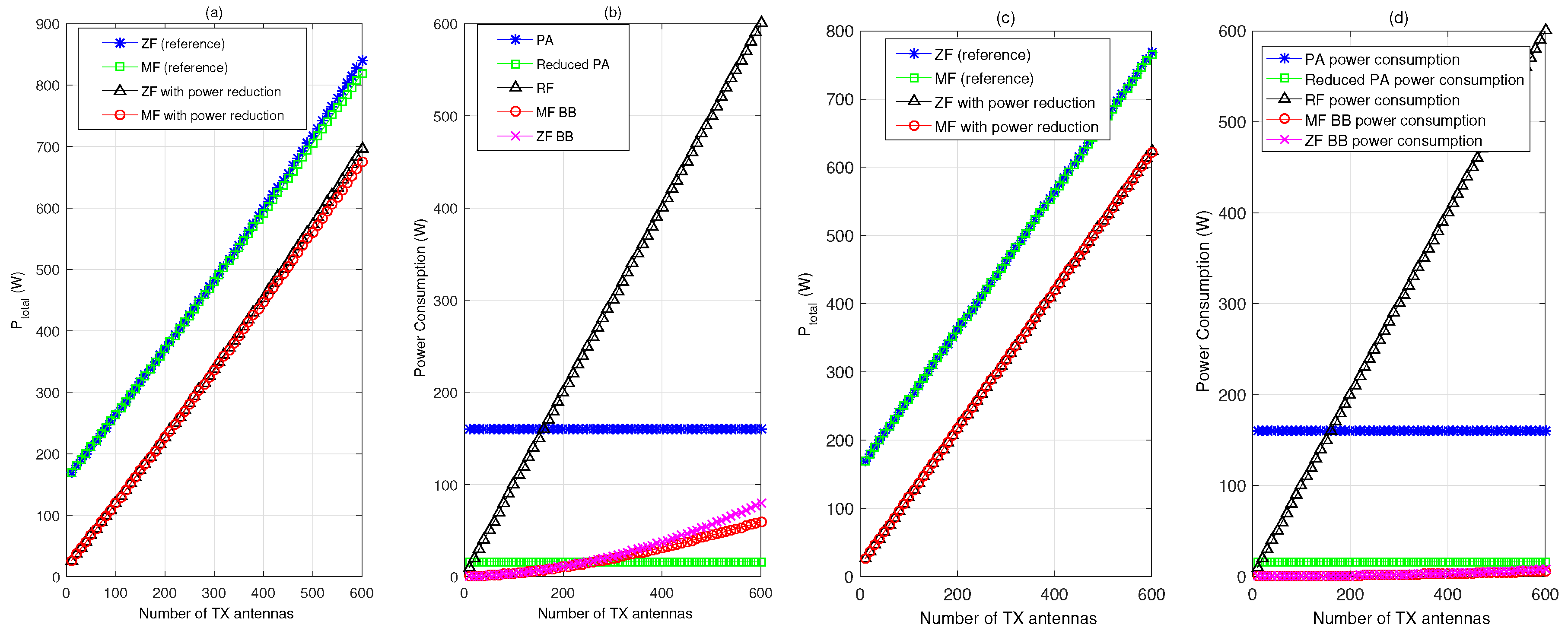
In Figure 8, we present the total power consumption and the power consumption of each component when the VLSI processing efficiency ϱ = 5 Gflop/W (Figure 8a,b), and 50 Gflop/W (Figure 8c,d), W, W and 4 W, K = 0.1 . The number of TX antennas ranges up to . As shown in the figure, increases linearly as the number of TX antennas increases. Here, the power reduction indicates a reduction in the PA power consumption by a factor of 10, i.e., from 160 W to 16 W. Choosing different algorithms for BB processing is not very helpful in reducing the , as shown in Figure 8. One more interesting thing is that the BB processing power consumption can take more power consumption than the PA power consumption, which is a very unusual case for current BS systems. From Figure 8a,b, the threshold point for this situation is when is more than 247 for ZF and 262 for MF. When the number of TX antennas is more than , the BB processing power consumption takes a greater portion than the reduced PA power consumption. When the BS has large amounts of TX antennas, the RF power consumption can take a greater portion than the PA power consumption in , as is well known. Even in the case of W, if the number of TX antennas is more than 160, the RF power consumption takes a greater portion than the PA power consumption in . The situation between the BB power consumption and the reduced PA power consumption can be different if the VLSI processing efficiency, ϱ, is higher than that of the previous case. In the case of ϱ = 50 Gflop/W, the BB processing power consumption is lower than the PA power consumption, even for , as shown in the right of Figure 8. All other characteristics in the case of ϱ = 50 Gflop/W are very much similar to those when ϱ = 5 Gflop/W.
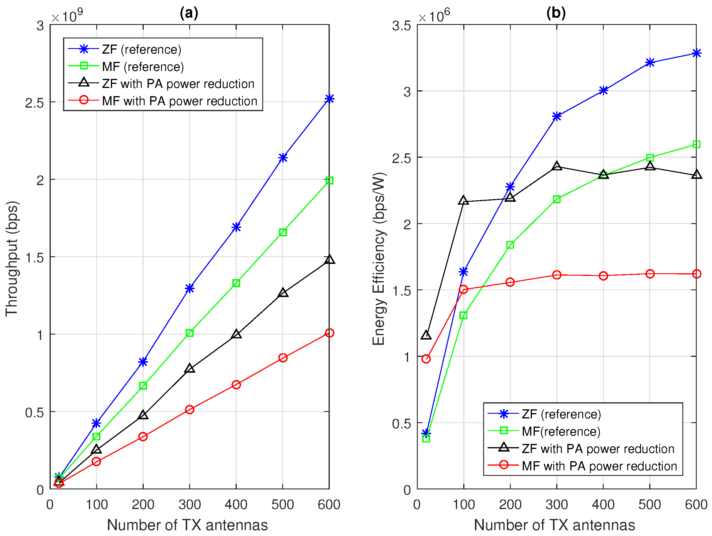
Now, let us look at the TP and EE based on the proposed BS structure. From now on, we use the case of ϱ = 50 Gflop/W. Figure 9 shows TP/EE versus the number of TX antennas. For the numerical simulations, we use a macro-cell type setup with a 2-GHz carrier frequency. The path loss in dB is modeled as 128.1 + 37.6 log(d) with distance d in kilometers [4,33]. We assume a cell radius of 2000 m with a cell-hole radius of 100 m. The coverage of LS-MIMO-quipped BS can be extended more due to the beamforming effect from the LS antenna systems. The user locations are uniform-random, and an average is taken over 100,000 trials. To show the effectiveness of the proposed algorithm and structure more dominantly, we present the results of user locations between 1000 and 2000 m. The LS-MIMO can cover a wider area due to the beamforming effect.
The results give us some important insight. First, when the number of TX antennas is relatively small, the PA power reduction provides further benefits for us in terms of the EE. Second, in contrast with the case of TP, in some regions, MF can provide a better EE than ZF. In future BS systems, it would also be quite general for the BS to only use a small portion of the equipped TX antennas by using an antenna selection scheme depending on the situation [16]. We can choose the ZF/MF/reference power/power reduction adaptively to improve the EE. The RSD-PS can help in this kind of work based on accumulated data. For example, to obtain the maximum EE with Figure 9, we choose ZF with a power reduction when the number of operating TX antennas is smaller than 190, and when the number of operating TX antennas is larger than 190, we choose the ZF reference.
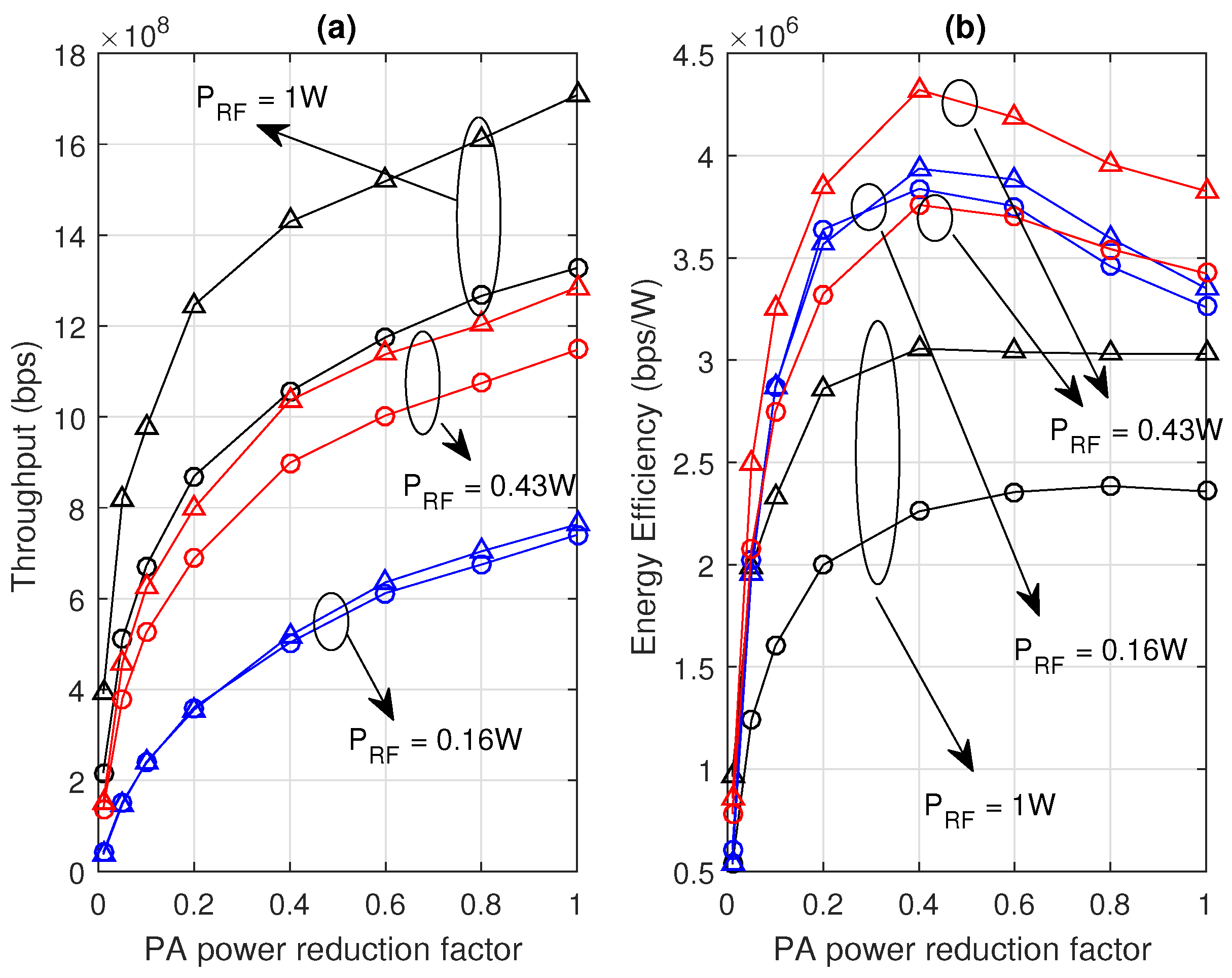
Now, let us fix some of parameters as , , ϱ = 50 Gflop/W, and W. In Figure 10, we present the total power consumption and power consumption of each component versus PA power reduction factor (Figure 10a,b) and TP and EE (Figure 10c,d).
We present the total power consumption and power consumption for each component versus the PA power reduction factor. Here, the PA power reduction factor refers to how much of the reference PA power consumption we use. For example, when the PA power reduction factor is 0.5, then we only use of the reference PA power consumption. If the PA power reduction factor is less than one, the RF power consumes more power than the PA power consumption.
If we observe the TP, it logarithmically increases as the PA reduction factor increases, i.e., the PA power consumption increases. This is quite obvious if we think of Shannon’s channel capacity characteristic. However, if we observe the EE, it increases until a certain point, and then, it decreases, even if we increase the PA power consumption. This is due to the fact that, after the maximum EE point, the increase in power consumption is faster than the increase in TP because the channel capacity does not increase so much, even if we increase the TX power, when it goes to the bandwidth-limited regime.
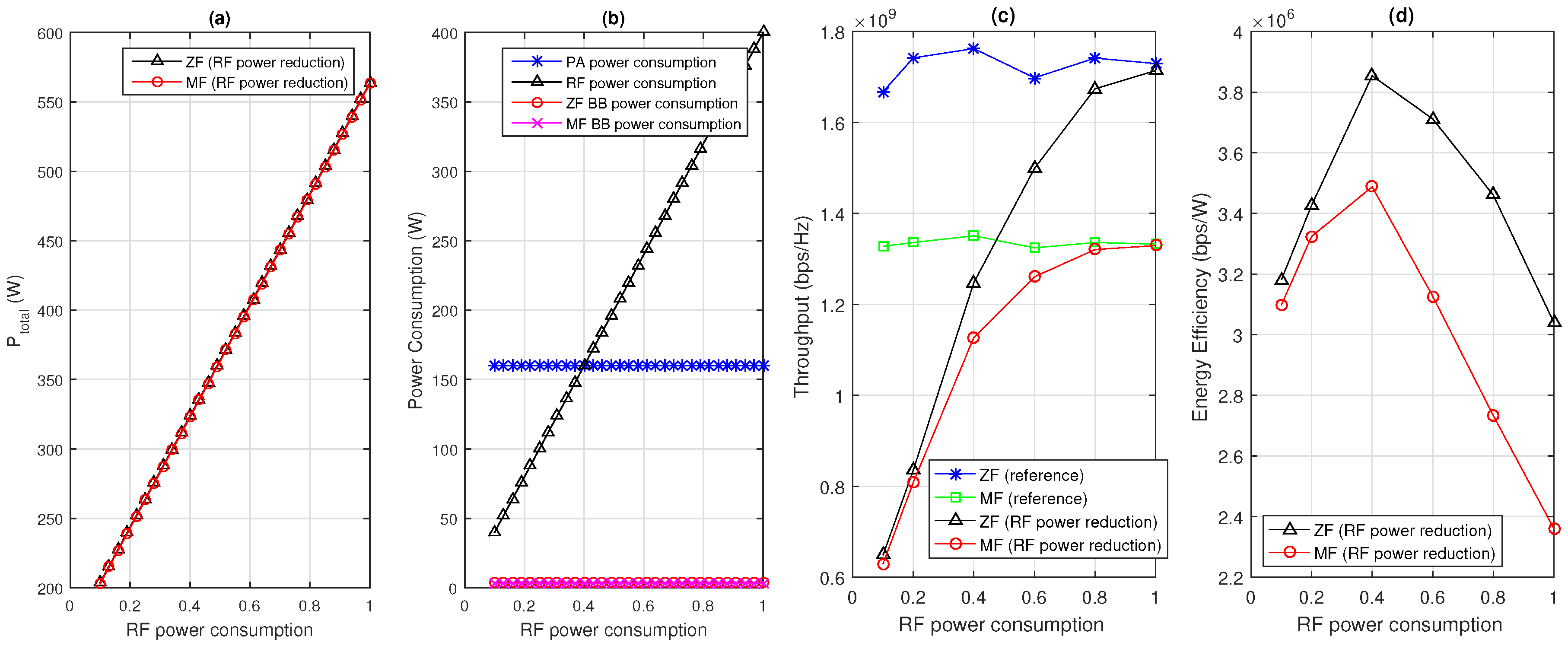
Keeping in mind the PA power adjustment case, now let us consider the RF power adjustment case. Figure 11 shows the total power consumption and power consumption of each component based on the RF power consumption between 0.1 W and 1 W, when and , VLSI efficiency Gflop/W and W. The total power consumption increases linearly as the RF power consumption increases. In this case, when the RF power consumes more than 0.4 W, it consumes more than the PA power consumption. To analyze the TP and EE, we use the RF power consumption model shown in Figure 1. As the RF power consumption increases, the TP also increases logarithmically for both ZF and MF. If we look at the EE, there are is a maximum EE point that can be achieved.
Based on the analysis to now, we finally show how much of a performance improvement is possible using the proposed BS. The PA power reduction factor versus TP/EE with variations in the RF power consumption and BB algorithm (ZF/MF) is presented in Figure 12. Each graph is the result of adjusting the BB/RF/PA power consumption. Figure 12 effectively shows how the performance changes by using the proposed BS structure since it shows the results of adjusting all three parameters in the proposed BS.
As shown in the figure, based on the proposed BS structure, we can adjust various parameters and choose the best TP/EE depending on the situation. The expected improvement in performance for the EE relative to the reference point (MF, PA power consumption factor = 1, W) is around ( bps/W), as summarized in Table 5.
5. Conclusions
In this paper, we proposed a BS structure that adjusts various parameters depending on the situation, as well as its corresponding systematic operation. The proposed BS includes an EE calculator unit and LUT based RSD-PS as the core components. It increases EE by using adjustable devices with a feedback scheme. Based on extensive simulations, the proposed BS is shown to give very flexible performance results to achieve a very high EE. Even though this scheme is proposed for use in a BS, it is quite general and can be applied to any kind of TX system.
Acknowledgments
This work was supported by the faculty research fund of Sejong University in 2016. This work was conducted by the research Grant of Kwangwoon University in 2016.
Author Contributions
Byung Moo Lee designed the algorithm, performed the simulations and prepared the manuscript. Youngok Kim was responsible for coordinating, writing and revising the paper. Both authors discussed the results and approved the publication.
Conflicts of Interest
The authors declare no conflict of interest.
References
- Wu, J.; Zhang, Y.; Zukerman, M.; Yung, E.K.N. Energy-efficient base-stations sleep-mode techniques in green cellular networks: A survey. IEEE Commun. Surv. Tutor. 2015, 17, 803–826. [Google Scholar] [CrossRef]
- Han, F.; Safar, Z.; Lin, W.S.; Chen, Y.; Liu, K.R. Energy-efficient cellular network operation via base station cooperation. In Proceedings of the IEEE International Conference on Communications (ICC), Ottawa, ON, Canada, 10–15 June 2012; pp. 4374–4378.
- Choi, H.H.; Lee, J.R. A Biologically-Inspired Power Control Algorithm for Energy-Efficient Cellular Networks. Energies 2016, 9, 161. [Google Scholar] [CrossRef]
- Tervo, O.; Le-Nam, T.; Markku, J. Optimal energy-efficient transmit beamforming for multi-user MISO downlink. IEEE Trans. Signal Process. 2015, 63, 5574–5588. [Google Scholar] [CrossRef]
- Tervo, O.; Tölli, A.; Juntti, M.; Tran, L.N. Energy-efficient coordinated beamforming with rate dependent processing power. In Proceedings of the 2016 IEEE 17th International Workshop on Signal Processing Advances in Wireless Communications (SPAWC), Edinburgh, UK, 3–6 July 2016.
- Cavalcante, R.L.; Stanczak, S.; Schubert, M.; Eisenblaetter, A.; Türke, U. Toward Energy-Efficient 5G Wireless Communications Technologies: Tools for decoupling the scaling of networks from the growth of operating power. IEEE Signal Process. Mag. 2014, 31, 24–34. [Google Scholar] [CrossRef]
- Holtkamp, H.; Auer, G.; Bazzi, S.; Haas, H. Minimizing Base Station Power Consumption. IEEE J. Sel. Areas Commun. 2014, 32. [Google Scholar] [CrossRef]
- Debaillie, B.; Giry, A.; Gonzalez, M.J.; Dussopt, L.; Li, M.; Ferling, D.; Giannini, V. Opportunities for energy savings in pico/femto-cell base-stations. In Proceedings of the Future Network & Mobile Summit (FutureNetw), Warsaw, Poland, 15–17 June 2011.
- Niu, Z.; Guo, X.; Zhou, X.; Kumar, P.R. Characterizing Energy–Delay Tradeoff in Hyper-Cellular Networks With Base Station Sleeping Control. IEEE J. Sel. Areas Commun. 2015, 33, 641–650. [Google Scholar] [CrossRef]
- Zhao, G.; Chen, S.; Zhao, L.; Hanzo, L. A Tele-Traffic-Aware Optimal Base-Station Deployment Strategy for Energy-Efficient Large-Scale Cellular Networks. IEEE Access 2016, 4, 2083–2095. [Google Scholar] [CrossRef]
- Björnson, E.; Sanguinetti, L.; Hoydis, J.; Debbah, M. Optimal design of energy-efficient multi-user MIMO systems: Is massive MIMO the answer? IEEE Trans. Wirel. Commun. 2015, 14, 3059–3075. [Google Scholar] [CrossRef]
- Pollakis, E.; Cavalcante, R.L.; Stańczak, S. Base station selection for energy efficient network operation with the majorization-minimization algorithm. In Proceedings of the IEEE 13th International Workshop on Signal Processing Advances in Wireless Communications, Cesme, Turkey, 17–20 June 2012; pp. 219–223.
- Li, M.; Chen, P.; Gao, S. Cooperative Game-Based Energy Efficiency Management over Ultra-Dense Wireless Cellular Networks. Sensors 2016, 16, 1475. [Google Scholar] [CrossRef] [PubMed]
- Jeong, J.; Kim, H. On Optimal Cell Flashing for Reducing Delay and Saving Energy in Wireless Networks. Energies 2016, 9, 768. [Google Scholar] [CrossRef]
- Chung, Y.-L. A Novel Power-Saving Transmission Scheme for Multiple-Component-Carrier Cellular Systems. Energies 2016, 9, 265. [Google Scholar] [CrossRef]
- Lee, B.M.; Choi, J.; Bang, J.; Kang, B. An energy efficient antenna selection for large scale green MIMO systems. In Proceedings of the 2013 IEEE International Symposium on Circuits and Systems (ISCAS2013), Beijing, China, 19–23 May 2013; pp. 950–953.
- Gimenez, S.; Roger, S.; Baracca, P.; Martín-Sacristán, D.; Monserrat, J.F.; Braun, V.; Halbauer, H. Performance Evaluation of Analog Beamforming with Hardware Impairments for mmW Massive MIMO Communication in an Urban Scenario. Sensors 2016, 16, 1555. [Google Scholar] [CrossRef] [PubMed]
- Jabbar, S.Q.; Li, Y. Analysis and Evaluation of Performance Gains and Tradeoffs for Massive MIMO Systems. Appl. Sci. 2016, 6, 268. [Google Scholar] [CrossRef]
- Marzetta, T.L. Massive MIMO: An Introduction. Bell Labs Tech. J. 2015, 20, 11–22. [Google Scholar] [CrossRef]
- Bjrnson, E.; Larsson, E.G.; Marzetta, T.L. Massive MIMO: Ten myths and one critical question. IEEE Commun. Mag. 2016, 54, 114–123. [Google Scholar] [CrossRef]
- Arnold, O.; Richter, F.; Fettweis, G.; Blume, O. Power Consumption Modeling of Different Base Station Types in Heterogeneous Cellular Networks. In Proceedings of the ICT MobileSummit (ICT Summit’10), Florence, Italy, 16–18 June 2010.
- Lee, B.M.; de Figueiredo, R.J.P. Adaptive Predistorters for Linearization of High-Power Amplifiers in OFDM Wireless Communications. Circuits Syst. Signal Process. 2006, 25, 59–80. [Google Scholar] [CrossRef]
- Cripps, S.C. RF Power Amplifiers for Wireless Communications, 2nd ed.; Artech House Publishers: Norwood, MA, USA, 2006. [Google Scholar]
- Miller, S.L.; O’Dea, R.J. Peak power and bandwidth efficient linear modulation. IEEE Trans. Commun. 1998, 46, 1639–1648. [Google Scholar] [CrossRef]
- Kumar, R.V.R.; Gurugubelli, J. How green the LTE technology can be? In Proceedings of the 2nd International Conference on Wireless Communication, Vehicular Technology, Information Theory and Aerospace & Electronic Systems Technology (Wireless VITAE), Chennai, India, 28 February–3 March 2011.
- Yang, H.; Marzetta, T. Performance of Conjugate and Zero-Forcing Beamforming in Large-Scale Antenna Systems. IEEE J. Sel. Areas Commun. 2013, 31, 172–179. [Google Scholar] [CrossRef]
- Yang, H.; Marzetta, T. Total energy efficiency of cellular large scale antenna system multiple access mobile networks. In Proceedings of the IEEE Online Conference on Green Communications (GreenCom), Beijing, China, 29–31 October 2013; pp. 27–32.
- Yang, H.; Marzetta, T. Energy efficient design of massive MIMO: How many antennas? In Proceedings of the 2015 IEEE 81st Vehicular Technology Conference (VTC Spring), Glasgow, UK, 11–14 May 2015.
- Marzetta, T.L. Noncooperative Cellular Wireless with Unlimited Numbers of Base Station Antennas. IEEE Trans. Wirel. Commun. 2010, 9, 3590–3600. [Google Scholar] [CrossRef]
- Dahlman, E.; Parkvall, S.; Skold, J. 4G: LTE/LTE-Advanced for Mobile Broadband; Academic Press: Salt Lake City, UT, USA, 10 May 2011. [Google Scholar]
- Spencer, Q.H.; Swindlehurst, A.L.; Haardt, M. Zero-Forcing Methods for Downlink Spatial Multiplexing in Multiuser MIMO Channels. IEEE Trans. Signal Proc. 2004, 52, 461–471. [Google Scholar] [CrossRef]
- Peel, C.B.; Hochwald, B.M.; Swindlehurst, A.L. A Vector-Perturbation Technique for Near-Capacity Multiantenna Multiuser Communication—Part I: Channel Inversion and Regularization. IEEE Trans. Commun. 2005, 53, 195–202. [Google Scholar] [CrossRef]
- ETSI Technical Report 136.931 Radio frequency (RF) Requirements for LTE Pico Node B; Technical Report; ETSI: Sophia Antipolis, France, 2012.
Figure 1.
Radio frequency (RF) power consumption model.

Figure 2.
An example of a high level conceptual figure of a large-scale multiple-input multiple-output (LS-MIMO) system.
Figure 2.
An example of a high level conceptual figure of a large-scale multiple-input multiple-output (LS-MIMO) system.
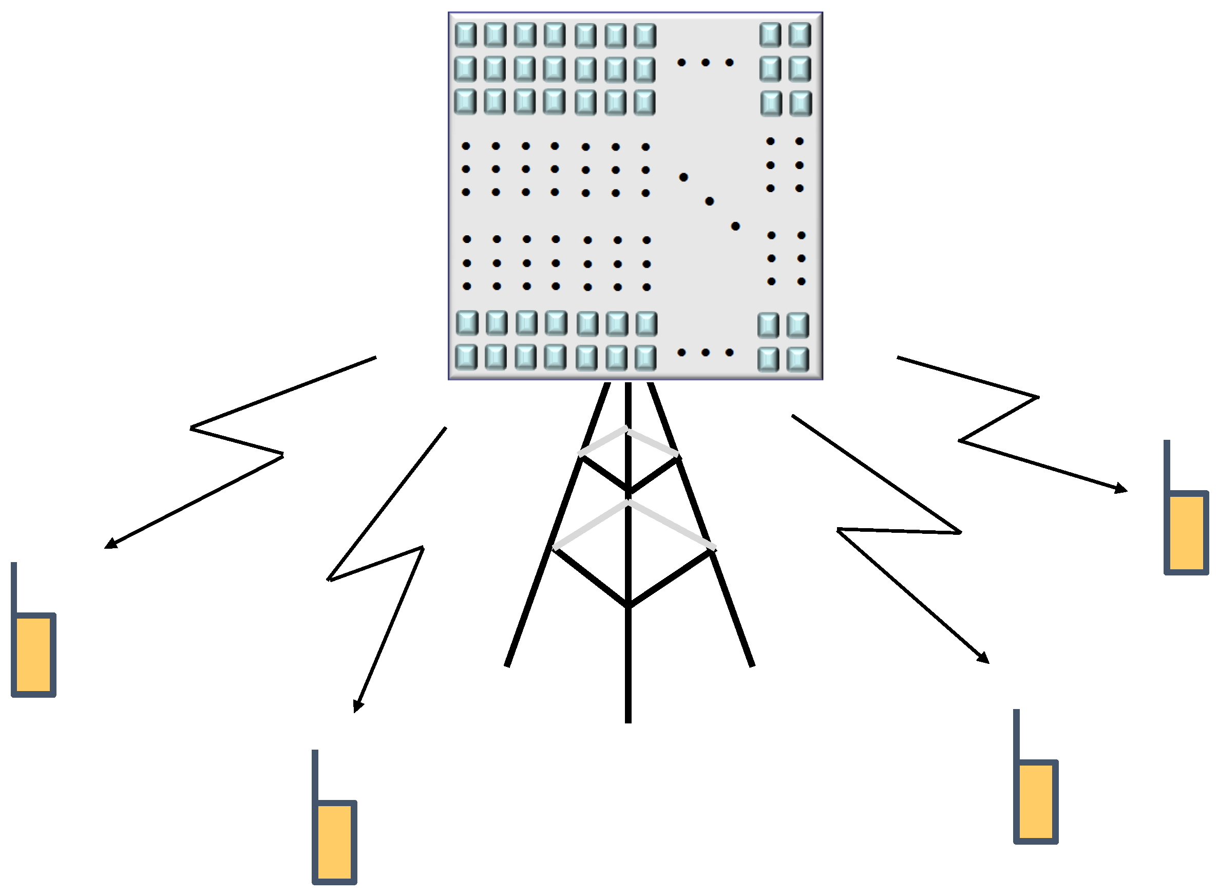
Figure 3.
An implementation example of the antenna and RF in an LS-MIMO system.

Figure 4.
The high level conceptual figure of the energy-efficient future base station (BS).

Figure 5.
Block diagram of the proposed BS structure.
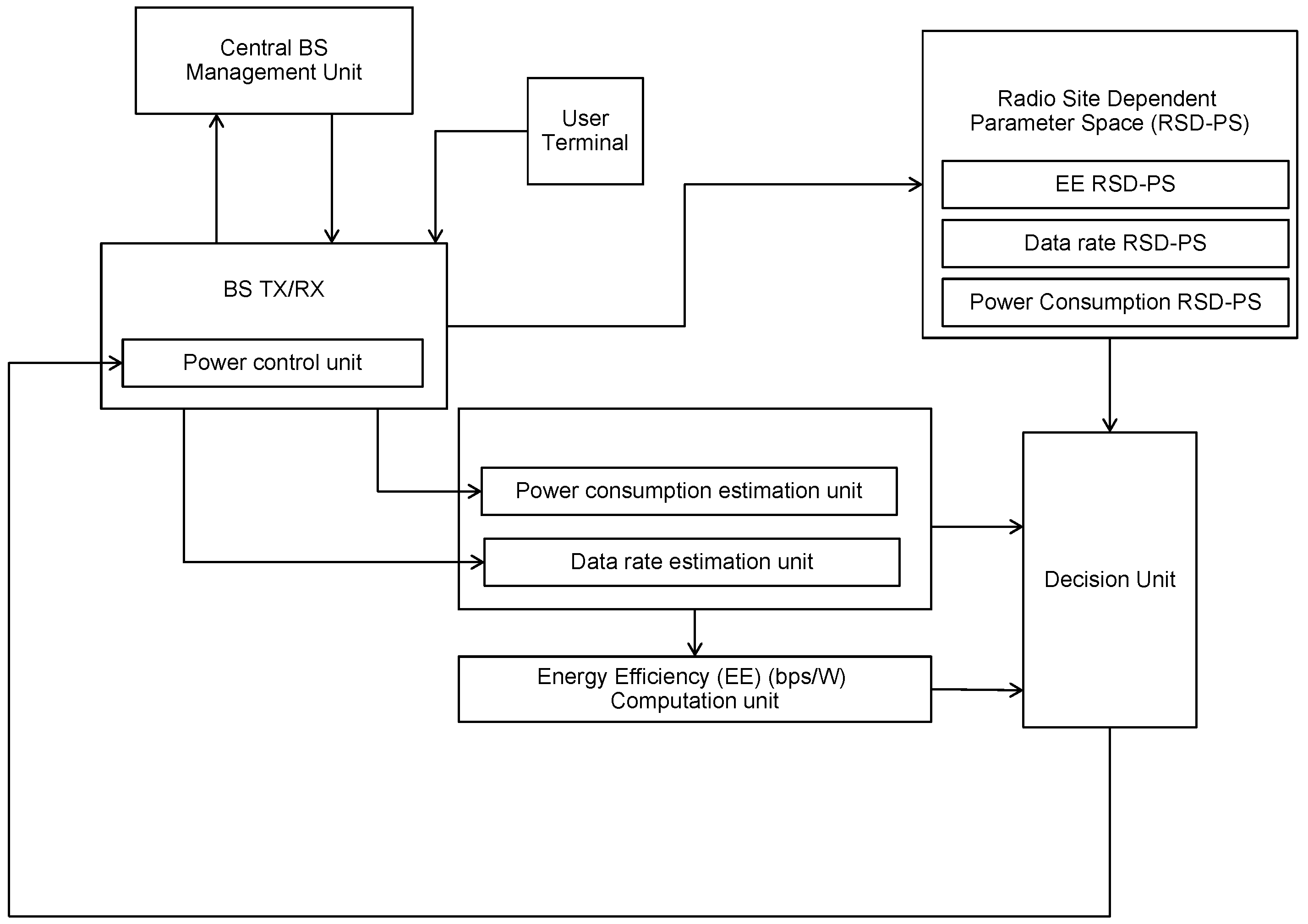
Figure 6.
Example of the systematic operation of the proposed BS.

Figure 7.
Reference BS structure used in the performance analysis.

Figure 8.
(a) total power consumption; and (b) power consumption of each component, when ϱ = 5 Gflop/W, W, W and 4 W, K = 0.1 ; (c) total power consumption; and (d) power consumption of each component, when ϱ = 50 Gflop/W, W, W and 4 W, K = 0.1 .
Figure 8.
(a) total power consumption; and (b) power consumption of each component, when ϱ = 5 Gflop/W, W, W and 4 W, K = 0.1 ; (c) total power consumption; and (d) power consumption of each component, when ϱ = 50 Gflop/W, W, W and 4 W, K = 0.1 .

Figure 9.
(a) TP (bps); and (b) EE (bps/W), as the number of transmitter (TX) antennas increases, when ϱ = 50 Gflop/W, W, W and 4 W, K = 0.1 .
Figure 9.
(a) TP (bps); and (b) EE (bps/W), as the number of transmitter (TX) antennas increases, when ϱ = 50 Gflop/W, W, W and 4 W, K = 0.1 .

Figure 10.
(a) total power consumption; and (b) power consumption of each component based on PA reduction factor, when and , ϱ = 50 Gflop/W, and W; (c) TP; and (d) EE when and , 50 Gflop/W and W.
Figure 10.
(a) total power consumption; and (b) power consumption of each component based on PA reduction factor, when and , ϱ = 50 Gflop/W, and W; (c) TP; and (d) EE when and , 50 Gflop/W and W.
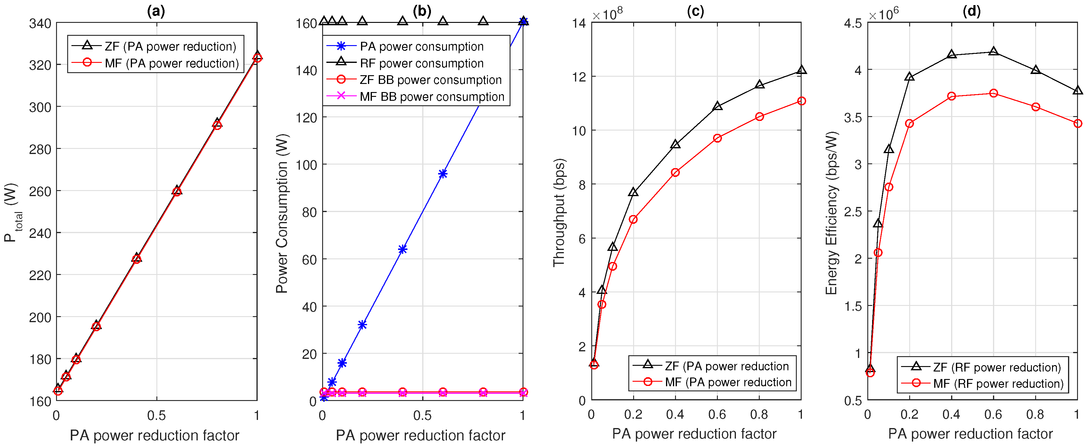
Figure 11.
(a) total power consumption; and (b) power consumption of each component based on RF power consumption, when and , 50 Gflop/W, and W; (c) TP (bps); and (d) EE (bps/W) based on RF power consumption, when and , 50 Gflop/W and W.
Figure 11.
(a) total power consumption; and (b) power consumption of each component based on RF power consumption, when and , 50 Gflop/W, and W; (c) TP (bps); and (d) EE (bps/W) based on RF power consumption, when and , 50 Gflop/W and W.

Figure 12.
Performance of proposed BS with various parameter adjustments: (a) TP (bps); and (b) EE (bps/W).
Figure 12.
Performance of proposed BS with various parameter adjustments: (a) TP (bps); and (b) EE (bps/W).


| Parameters | Description | Power Consumption |
|---|---|---|
| B | Bandwidth | 10 MHz |
| Slot length | ms | |
| Pilot length in one slot | ms | |
| Symbol duration | 71.4 μs | |
| GI | 4.7 μs | |
| Symbol without GI | 66.7 μs | |
| Delay spread | 4.7 μs |
Table 2.
The precoding matrices of matched filtering (MF), zero-forcing (ZF) and regularized zero-forcing (RZF).
| MF | ZF | RZF | |
|---|---|---|---|
| Operation Metrics | Parameters |
|---|---|
| Data Rate | Channel Information (from Terminal) |
| System Bandwidth (from BS) | |
| Radiation power (from BS) | |
| Number of Operating TXantenna (from BS) | |
| Number of Co-Scheduled User Terminals (from BS) | |
| Power Consumption | PA power consumption (from BS) |
| RF power consumption (from BS) | |
| BB power consumption (from BS) |
| (1) | Method to increase TP while decreasing EE |
| (2) | Method to increase EE while decreasing TP |
| (3) | Method to maintain EE while increasing TP |
| (4) | Method to maintain TP while decreasing EE |
| (5) | Method to increase both TP and EE and increase TP further |
| (6) | Method to decrease both TP and EE and decrease EE further |
| References | EE Improvement (%) |
|---|---|
| From ZF reference | ( Mbps/W) |
| From MF reference | ( Mbps/W) |
© 2016 by the authors; licensee MDPI, Basel, Switzerland. This article is an open access article distributed under the terms and conditions of the Creative Commons Attribution (CC-BY) license (http://creativecommons.org/licenses/by/4.0/).
Share and Cite
MDPI and ACS Style
Lee, B.M.; Kim, Y. Design of an Energy Efficient Future Base Station with Large-Scale Antenna System. Energies 2016, 9, 1083. https://doi.org/10.3390/en9121083
AMA Style
Lee BM, Kim Y. Design of an Energy Efficient Future Base Station with Large-Scale Antenna System. Energies. 2016; 9(12):1083. https://doi.org/10.3390/en9121083
Chicago/Turabian StyleLee, Byung Moo, and Youngok Kim. 2016. "Design of an Energy Efficient Future Base Station with Large-Scale Antenna System" Energies 9, no. 12: 1083. https://doi.org/10.3390/en9121083
Note that from the first issue of 2016, this journal uses article numbers instead of page numbers. See further details here.