Article

Artificial Neural Network Model for Alkali-Surfactant-Polymer Flooding in Viscous Oil Reservoirs: Generation and Application

Department of Energy Resources Engineering, Inha University, Incheon 402-751, Korea
*
Author to whom correspondence should be addressed.
Energies 2016, 9(12), 1081; https://doi.org/10.3390/en9121081
Submission received: 20 October 2016 / Revised: 9 December 2016 / Accepted: 13 December 2016 / Published: 17 December 2016

Abstract

:
Chemical flooding has been widely utilized to recover a large portion of the oil remaining in light and viscous oil reservoirs after the primary and secondary production processes. As core-flood tests and reservoir simulations take time to accurately estimate the recovery performances as well as analyzing the feasibility of an injection project, it is necessary to find a powerful tool to quickly predict the results with a level of acceptable accuracy. An approach involving the use of an artificial neural network to generate a representative model for estimating the alkali-surfactant-polymer flooding performance and evaluating the economic feasibility of viscous oil reservoirs from simulation is proposed in this study. A typical chemical flooding project was referenced for this numerical study. A number of simulations have been made for training on the basis of a base case from the design of 13 parameters. After training, the network scheme generated from a ratio data set of 50%-20%-30% corresponding to the number of samples used for training-validation-testing was selected for estimation with the total coefficient of determination of 0.986 and a root mean square error of 1.63%. In terms of model application, the chemical concentration and injection strategy were optimized to maximize the net present value (NPV) of the project at a specific oil price from the just created ANN model. To evaluate the feasibility of the project comprehensively in terms of market variations, a range of oil prices from 30 $/bbl to 60 $/bbl referenced from a real market situation was considered in conjunction with its probability following a statistical distribution on the NPV computation. Feasibility analysis of the optimal chemical injection scheme revealed a variation of profit from 0.42 $MM to 1.0 $MM, corresponding to the changes in oil price. In particular, at the highest possible oil prices, the project can earn approximately 0.61 $MM to 0.87 $MM for a quarter five-spot scale. Basically, the ANN model generated by this work can be flexibly applied in different economic conditions and extended to a larger reservoir scale for similar chemical flooding projects that demand a quick prediction rather than a simulation process.

1. Introduction

After a period of time of producing oil from natural energy reservoirs using primary and secondary extraction methods, enhanced oil recovery (EOR) methods are commonly considered to extract the large amounts of oil often remaining in reservoirs. The tertiary stage is basically categorized into three essential processes: thermal oil recovery, gas miscible/immiscible flooding, and chemical flooding [1]. Thermal methods are suitable for heavy-oil or bitumen, while gas injection is widely used where sufficient gas supplies are available. Most importantly, oil recovery by carbon dioxide injection requires specific reservoir conditions to maintain the optimal sweep efficiency [2], particularly the reservoir pressure must be continuously monitored to enhance the gas storage [3]. The favorability of chemical flooding methods, which include alkaline (A)-surfactant (S)-polymer (P) flooding, is that these methods can be operated continuously in conjunction with water flooding without any addition complex integrated system [4,5]. The application of chemical agents for extracting crude oil has been commercially deployed, not only for conventional light oil, but also in some viscous oil fields over the world. Indeed, according to the reports of the journal Oil & Gas, the successful polymer flooding project in the Pelican Lake field in Canada could profitably produce more than 9540 m3/day in 2014, whereas the pilot project in the Gudong field also recovered approximately 13.4% of the original oil in place (OOIP) in 1998 by ASP flooding [6,7,8]. However, like other EOR methods, the successful application of chemical injections still depends on many factors including reservoir conditions, the type of crude oil or operating conditions, and most importantly the economic feasibility of the project.
Conventionally, core-flood tests and simulations are always considered to forecast the EOR performance of chemical flooding before deploying it in a real field. On the other hand, the large time consumed and high cost are always in concerns because injection jobs inevitably have high uncertainty. Further, an injection strategy is essential to achieve optimization of either the technical or economic aspects [9]. With a low number of numerical simulations, the optimization methodology proposed by Zerpa et al. for a full field scale was used to investigate surrogate models for two ASP flooding scenarios and could be applied more generally to other ASP injection scenarios [10]. Their later work demonstrated the use of response surface methodology (RSM) as an effective optimization tool for an ASP pilot project with the optimal polymer slug size 68.6% smaller than that suggested by laboratory design [11]. In addition to chemical flooding, this mathematical tool has been also widely applied in other EOR processes for diverse professional analyses. Dai et al. conducted a response surface analysis for two objective functions using the results of 2000 Monte Carlo simulations for optimizing the CO2-EOR process; they implied that understanding the uncertainty of the reservoir characterization would be critical in terms of economic decision and cost-effectiveness of the process [12]. Their subsequent work proposed a response surface-based economic model to compute the profitability of CO2-EOR for the Farnsworth Unit site taking into account the oil price; they stated the importance of oil price on the possibility of profit from 1000 realizations [13]. Principally, a more proper prediction made by RSM, a larger number of designed samples is required, especially when a large number of variables is involved in the response function [14].
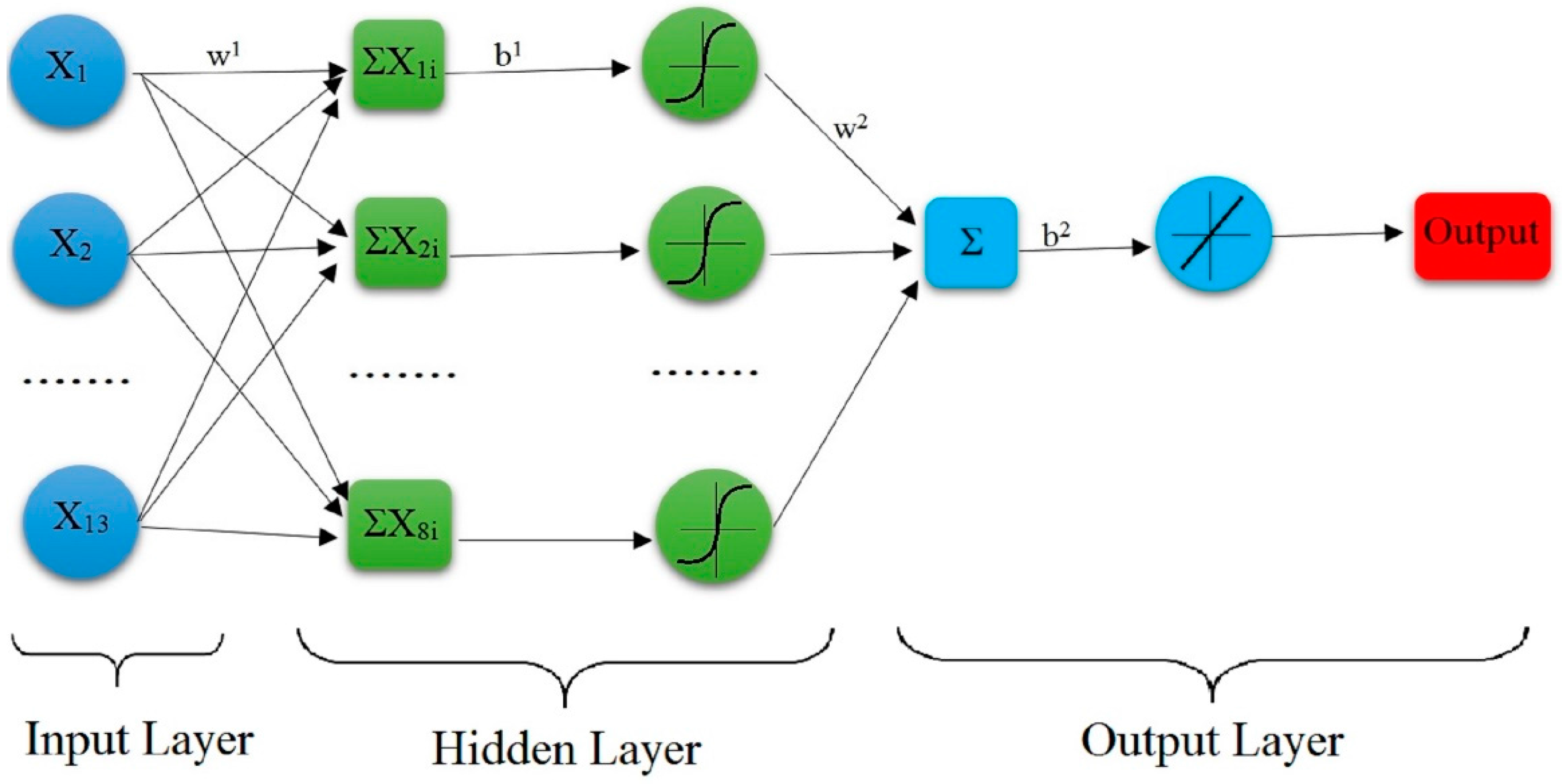
The artificial neural network (ANN) has been applied widely in many aspects of the petroleum industry, but despite the diversity of its applications, there have been few studies of this method in chemical flooding. Using an ANN, Jawad and Jreou determined the horizontal well location in the AB unit of South Rumaila oil field with reasonable accuracy; they also affirmed the value of this tool for cases with a large amount of historical data rather than adequate engineering data [15]. Instead of analyzing and predicting the production data by decline curves, Elmabrouk et al. utilized network models to match the history production data and provide an estimation from those data sets of an oil field in the Sirte Basin in Libya with a mean absolute error of approximately 10% [16]. Further, the accurate estimation for horizontal well production performance by ANN to calculate the pseudo skin factor by Ahmadi et al. opened a potential coupling of their suggested model with commercial software to improve the accuracy and decrease the simulation time [17]. Regarding EOR processes, Alizadeh et al. pointed out the superior prediction of ANN on predicting the oil recovery factor in the immiscible water alternating gas process compared to a mathematic tool [18]. Their later work also on three-phase fluids flow in heterogeneous porous media affirmed the applicability of the ANN model based on the Scaling Group for accurately estimating the oil recovery potential in any given reservoir. In particular, the method can be useful for detecting the key parameters in a large database for immiscible WAG flooding [19]. Beside the network model, an optimization tool also needs to be integrated for fully evaluating the performance of the models and figuring out the most dominant screening values in achieving the target. Shafiei and Dusseault developed a new screening tool based on ANN integrated with a Particle Swarm Optimization (PSO) method to predict recovery factors and cumulative steam to oil ratios in steam flooding for viscous oil in naturally fractured carbonate reservoirs, potentially opening the possibility of merging PSO-ANN with viscous oil recovery modeling software [20]. They demonstrated that PSO-ANN is superior to BP-ANN at forecasting in this type of oil field with the maximum error of less than 8%.
In terms of chemical flooding, Wang et al. constructed EOR and IPR models for polymer flooding in reservoir blocks of the Shengli oil field by orthogonal design and a BP neural network with three oil prices; the model could potentially supply technical guidance for polymer injection implementation [21]. Moreover, the ANN model for surfactant-polymer flooding has been built successfully with approximately 3% average absolute error from a set of 499 simulation data with 18 dimensionless groups involved in the input layer by Al-Dousari and Garrouch; they clearly stated that the model can save significant time in performance prediction compared to the simulation on SP flooding with reliable accuracy [22].
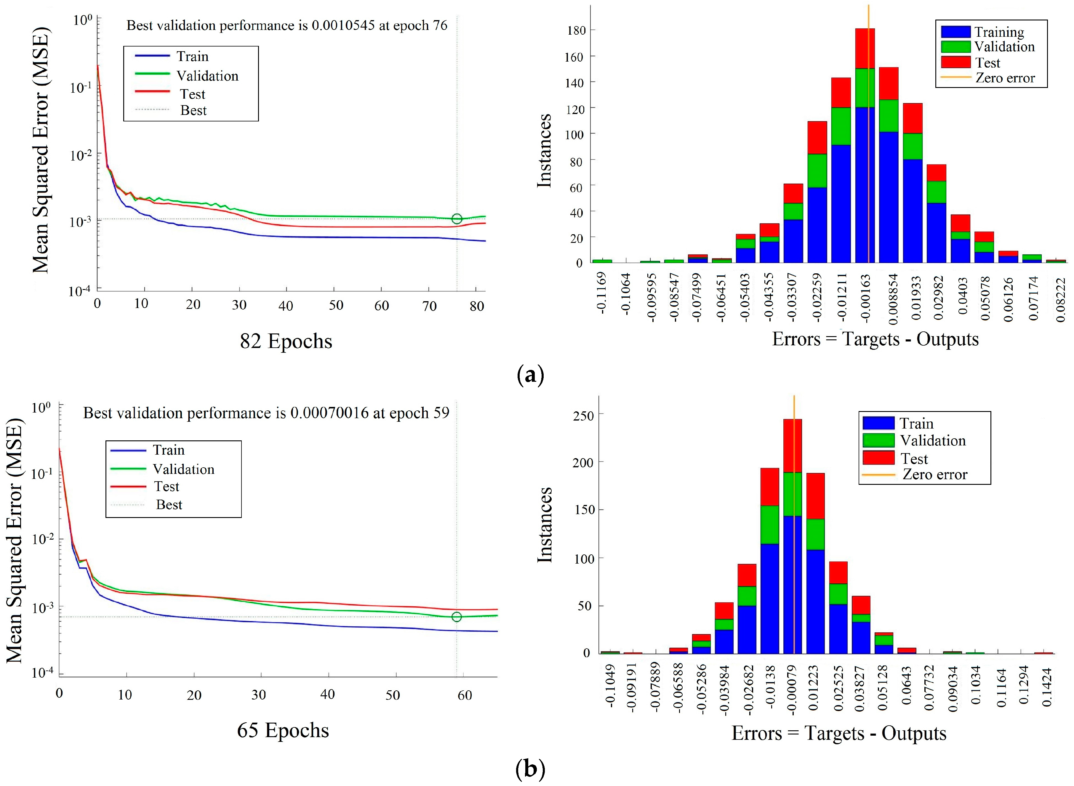
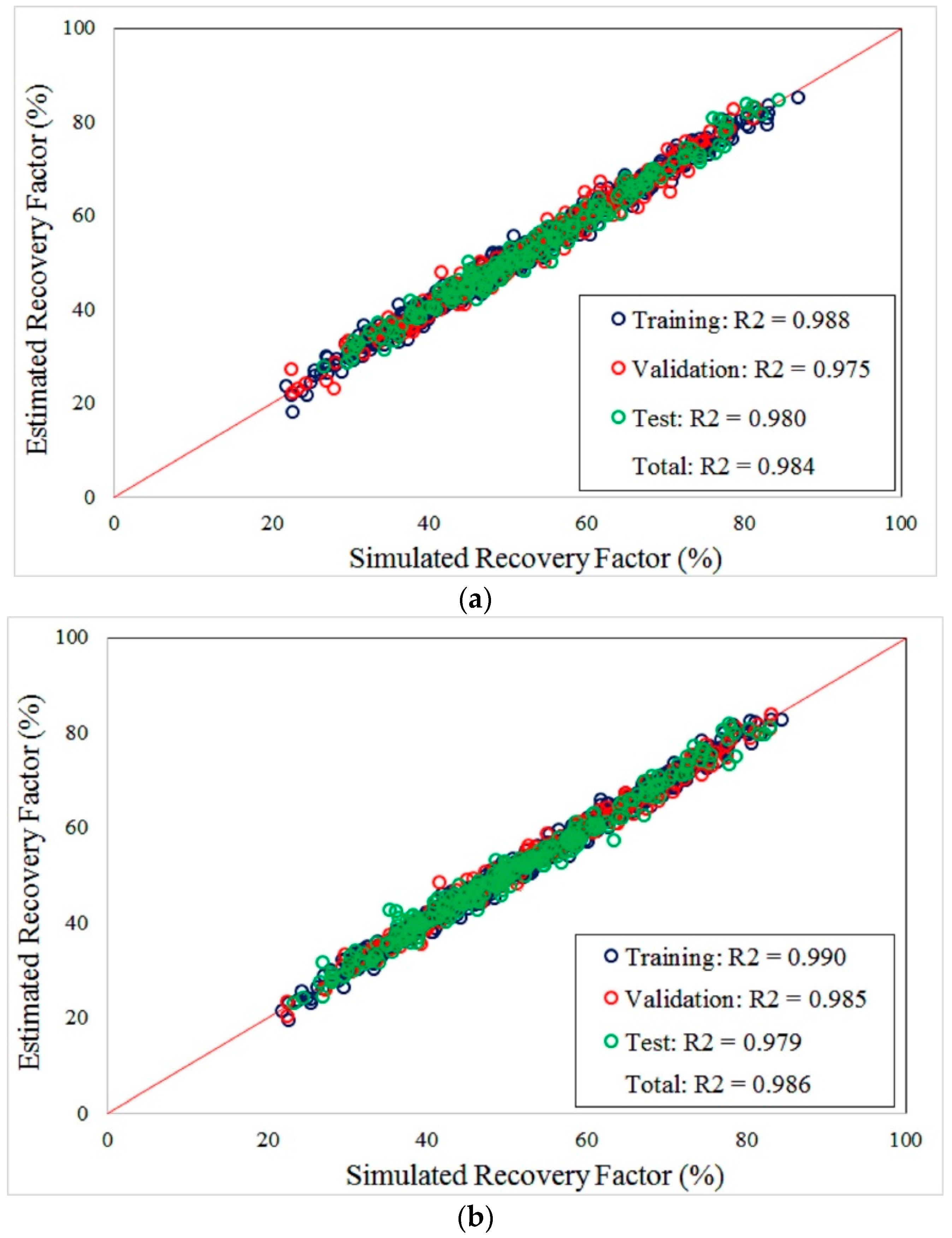
Obviously, while the applications of a neural network are diverse and highly applicable, as presented in the literature there is still no representative model for estimation of the viscous oil reservoir situation as the use of chemical flooding in this type of oilfield has not been widely considered. Based on the abovementioned idea, this work aimed to generate an applicable network model to predict the ultimate oil recovery of chemical flooding process in a quarter five-spot pattern for a viscous oil reservoir. The numerical case study is referenced from a typical ASP flooding project in China, a validation for simulation in terms of chemical designs will be also presented in order to assure the reliability of the work. A huge number of samples collected from simulation results will be used to train the neural network, a best scheme of training will be also determined to achieve the most reliable model. Sensitivity and feasibility studies in terms of economic evaluation are proposed as the applications of the generated network model in which the oil prices are notably considered that represents the risk of economic condition.
The generated ANN model in this work can absolutely be reused in similar projects that basically have similar reservoir characteristics where there is a need to quickly predict the possible recovery factor for ASP flooding, particularly for further feasibility analysis that can also be flexibly carried out for different economic conditions.

2. Reservoir Description

This study uses for analysis numerical data in which the reservoir model and injection strategy were mainly referenced from a typical successful pilot ASP flooding project in the Gudong oil field in China [8,23] (Table 1).
In detail, the real project consisted of four injectors and nine producer wells in a four inverted five-spot pattern with an area of 30,977 m2 and a net thickness of 11 m; the designed well distance was 50 m. From this practical information, this paper proposes a relatively similar reservoir model at a quarter five-spot pattern scale with one producer and one injection well that is built entirely in a STARS (CMG) simulator. The permeability of the reservoir varies downward with a factor of 0.33 and heterogeneously within a layer in sandstone rock system. However, presumably the insignificant difference of permeability between layers will not remarkably influence the flooding performances, particularly in a thin reservoir [24]. The other parameters are almost identical to those of the real Gudong field.
According to Dusseault and Shafiei, viscous oil is defined as crude oil which has viscosity ranging from 100 to 10,000 cp or specific gravity lower than 20 °API [25]. Therefore, despite the fact the oil viscosity is just 41.3 cp, the crude oil in this study can be considered as viscous since it has 17.45 °API; in other words, this work absolutely considers a high viscosity oil reservoir.

3. Chemical Injection Design

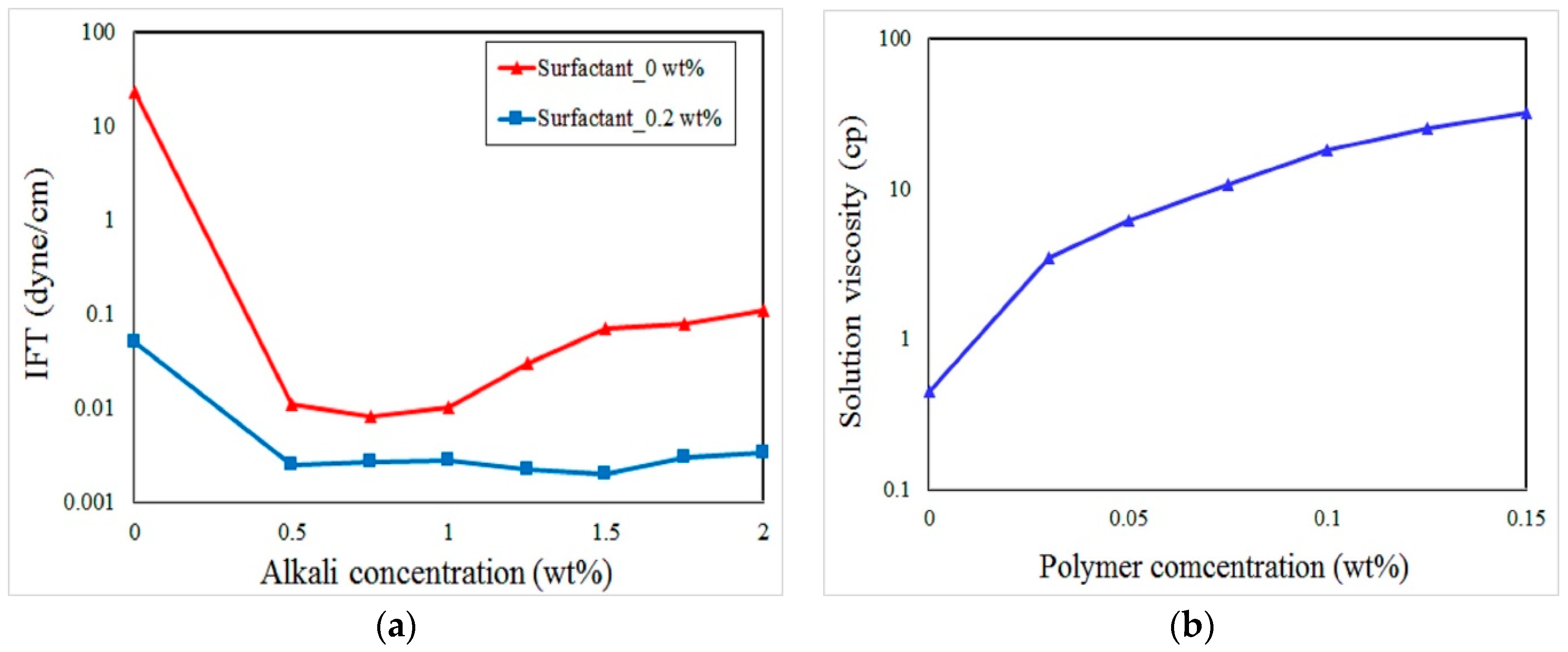
Basically, the use of alkali aims to generate a surfactant in-situ in the reservoir by reacting with the acid components of crude oil, thereby reducing the interfacial tension between the oil and the aqueous phases and making the oil moveable [26]. The addition of a synthetic surfactant to an alkali solution will increase the level of IFT reduction, but the combined alkali-surfactant injection can easily cause a severe viscous channeling phenomenon because oil will be easily bypassed by the displacing fluid, thereby leaving behind a large amount of oil. This problem can be tackled principally by using a polymer that makes the solution more viscous, thereby achieving the proper mobility control and significantly improving the sweep efficiency [27,28]. On the other hand, a high viscosity solution has decreased injectivity and consequently this results in a slower response at the producing well compared to the case where non-viscous fluids are injected [29].
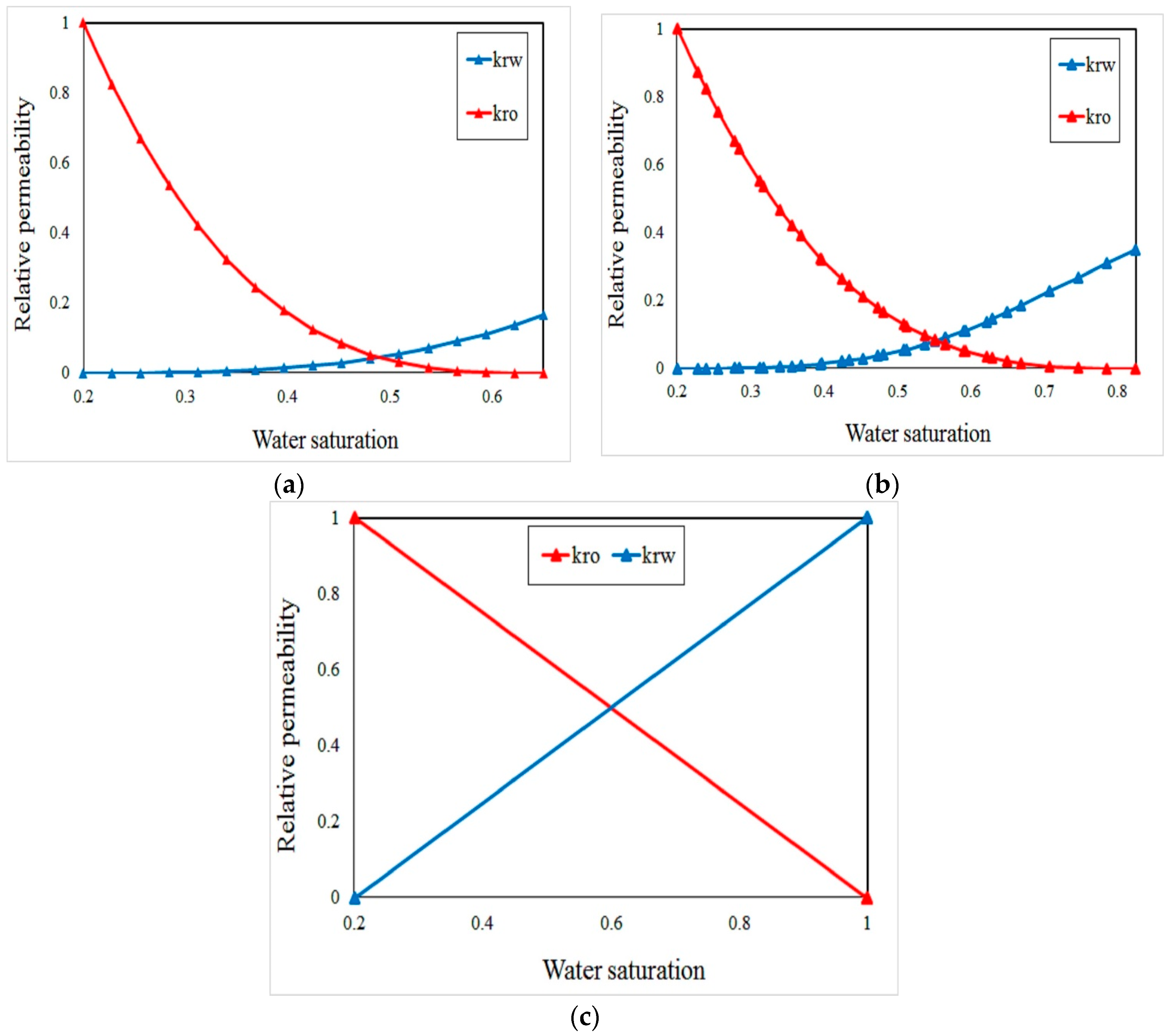
Regarding the simulation for chemical flooding, interpolation is basically the main numerical scheme of STARS for processing the variations in rock wettability, which is represented by the residual oil saturation, corresponding to the surfactant concentrations. This relationship originated fundamentally from the dependence of the residual saturation on the capillary number following the direct formula proposed by Pope and Nelson [30], as presented below:
S o r = a + b   log ( N c )
where a and b are constants, Sor is the residual oil saturation, and Nc is the capillary number. Obviously, since b is negative, the increase in capillary number primarily decreases Sor, which finally straightens the relative permeability curves. Quy and Labrid developed the mechanism of oil displacement according to the range of capillary numbers in surfactant flooding, as oil can be displaced totally if ln(Nc) > −6.725 and displaced partially if −8.255 < ln(Nc) < −6.725 [31]. The capillary number can be calculated as [32]:
N c = μ u / σ
where µ is the viscosity of the injected fluid, u is the Darcy velocity and σ is the interfacial tension between oil and water. As the IFT relationship is established initially for alkali and surfactant concentrations, it will be interpolated adaptably during the simulation processes. The interpolation of rock wettability in this work is represented by the changes in the relative permeability curves, as shown in Figure 1.
In terms of viscosity, the predefined viscosity table for an aqueous phase when adding a polymer will automatically generate a nonlinear mixing function, fN, which limits the polymer concentration during the simulation. The function is formulated as [32]:
f N = [ ln ( μ p ) ln ( μ w ) ] / [ ln ( μ p m a x ) ln ( μ w ) ]
where µw is the water viscosity, µp is the viscosity of polymer solution, and pmax is the maximum viscosity of the injected solution.
Effects of salinity on viscosity inevitably occur as this composition helps decide the quality of the microemulsion when the polymer and surfactant are mixed contemporarily in an artificial brine. In addition, because the reservoir water always has a certain level of salinity, the initial expected viscosity of the displacing fluid might not be reached as a consequence. The consideration of salinity in STARS is expressed basically as [32]:
μ p = μ p 0 ( x s a l t x min ) s p   for   x s a l t > x min ;   and   μ p = x p 0   for   x s a l t x min
where µp is the solution viscosity with salinity, μ p 0 is the defined viscosity of the polymer solution without salinity; xsalt and xmin are the salinity and effective threshold salinity of the solution, respectively; sp is the slope of the log-log plot of the polymer viscosity versus ratio of current salinity over xmin. The viscosity of polymer solution can be estimated more accurately before and during the simulation process because a specific salinity has been determined for artificial brine.
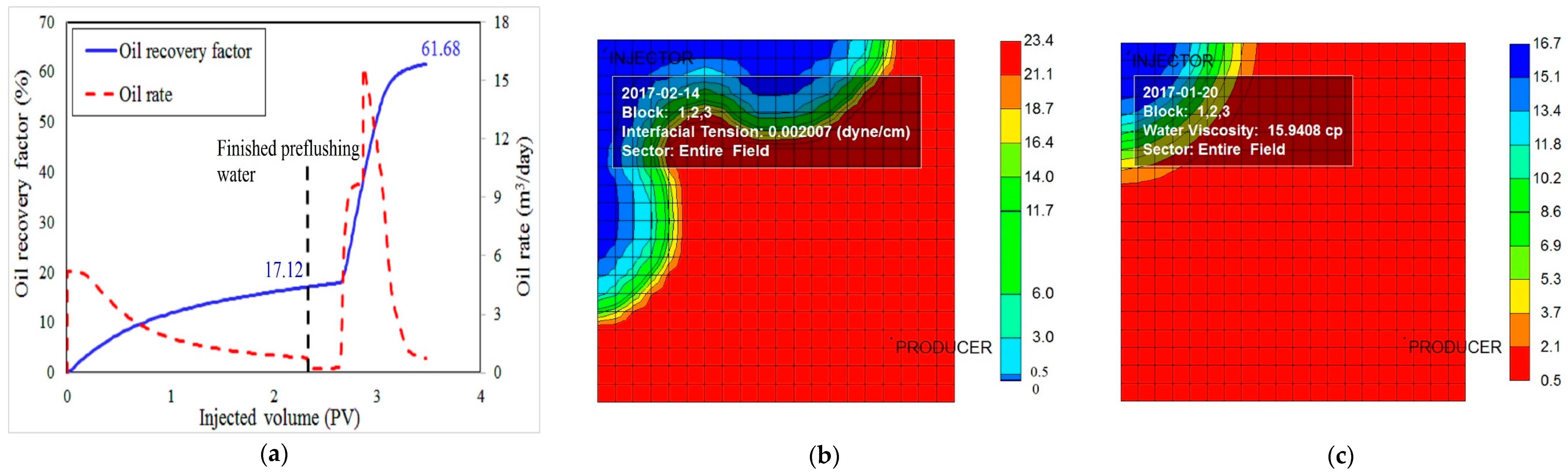
Based on the chemical properties, including IFT relationship, solution viscosity, and adsorption characteristics of the Gudong field project, this work applies these properties relatively completely for the simulation, as presented in Figure 2. Practically, a combined alkali-surfactant-polymer (ASP) is often considered instead of a single agent following a relevantly designed injection sequence to extract oil most thoroughly in terms of the technical or economic point of views [33]. As the flooding sequence of ASP injection in Gudong field has already been proven to be a typically effective sequence, this study also used the same injection strategy for the simulation. Table 2 provides details of the chemical injection schemes. Owing to the different scale between the real project and this work, the precise injection rate was redesigned based on the referenced rate by dividing the practical rate by 16. A preflushing water slug is also proposed before injecting the chemical slugs simultaneously.

4. ANN Model

4.1. ANN Structure

The applications of an ANN as a learning machine for estimating unavailable data from a sufficient amount of input and target samples by the network have been widely reported. The network normally consists of several layers, which can be an input layer, an output layer, and one or more hidden layers [34,35]. Fundamentally, the layers connect with each other by a linking system, which can be represented principally by weights, biases, and activating functions that are applied directly to the neurons of each layer [36]. Systematically, in a three-layer network, the neurons of the input layer connect with each neuron in the hidden layer through the specific weights, which indicates the contribution of the individual neurons in the input layer to that neuron in the hidden layer, and a transfer (activating) function with the existence of a bias value [37]. As all neurons of the hidden layers are generated, they connect directly with the output (final layer) by the same process. Figure 3 presents a schematic model of the ANN structure for data learning process of this work.
The ANN structure of this work is a multilayer neural network that has been applied successfully and demonstrated to be an effective learning machine schemer. A total of 13 parameters were set as 13 neurons in the input layer, including the alkali concentration in AS slug (A1), alkali concentration in the ASP slug (A2), polymer concentration in the first polymer slug (P1), polymer concentration in the ASP slug (P2), polymer concentration in the second polymer slug (P3), surfactant concentration in AS slug (S1), surfactant concentration in ASP slug (S2), first polymer slug size (P1_size), AS slug size (AS_size), ASP slug size (ASP_size), second polymer slug size (P3_size), slug size of preflushing water, and well distance.
First, the consideration of the water slug size can represent the influence of oil saturation in the reservoir on the flooding performance. Second, the well distance was first taken into account in this work as a parameter for examining the spatial effect on the oil production performance because it represents the well pattern design.
The hidden layer contains eight neurons connecting with its lower layer by weights and a transfer function:
a i 1 = t a n s i g ( y i + b i 1 ) ,   i = 1 8
with :   y i = j = 1 13 X i j ,   X i j = X j × w i j 1
where Xj represents the variable in the input layer, w i j 1 is the corresponding weight of the jth neuron of the input layer to connect with the ith neuron of the hidden layer, and b i 1 is bias value for the ith neuron in the hidden layer. The transfer function used on activation is a tan-sigmoid function as follows:
t a n s i g ( n ) =   2 1 + e 2 n 1
A linear relationship is proposed for the final link between the neurons in the hidden layer and the output, with connecting weights wi2 and bias b2 introduced correspondingly between the ith neuron and the output layer. Generally, NPV was normally considered for the output value. On the other hand, as the oil price is becoming more sensitive for the project, this work proposes the ultimate oil recovery factor (RF) as the output of the network instead of the NPV.

4.2. ANN Processing

A set of 988 samples from simulation results was used to process the ANN network in the MATLAB Network Toolbox. As the network pattern has been defined, the next important step is the division of the data set for training, validation, and testing under a back-propagation algorithm. Theoretically, this algorithm initiates with the first weight and bias vectors, and the output is then calculated from those initial values in the feedforward network. The error between simulated result and computed output is used to evaluate the accuracy of the estimation, weights and biases are then adjusted using the Levenberg-Marquardt algorithm, which is popularly used in the least squares curve fitting problem. This gradient descent formula is described as [38]:
x k + 1 = x k [ J T J + ω I ] 1 J T e
where x represents the values considered for adjustment (weights and biases), J is the Jacobian matrix that contains the first derivatives of the network errors, ω is a factor aiming to shift the formula toward Newton’s method, and e is a vector of the network errors. The weights and biases will be updated throughout the training process; principally, a more accurate network can be obtained with a larger volume of data for training [39,40]. On the other hand, as the use of an inadequate number of data for training can inevitably cause overfitting, which provides very high accuracy for estimating the training data but fails to perform in different data sets. In contrast, selecting insufficient data for training also does not fully adapt the network for the estimation. The validation data set is utilized mainly to tackle the problem of overfitting and underperformance by the early stopping technique. In other words, the technique targets to optimize the network performance by controlling the number of epochs, which represent the iteration process during training by ensuring the minimal errors of the system [41]. The testing data set is then used to test the validation of the network for completely blind data, which does not participate in the training process. Presumably, the large number of testing data being well fitted evidently performs the high accuracy of the network on predicting the unavailable data.
To determine the suitable data set division, this study verifies three ratio cases for training-validation-testing data including 60%-20%-20%, 55%-20%-25%, and 50%-20%-30%. The results were evaluated through the root mean square error (RMSE) and determination coefficient (R2), as formulated for the simulated target xi,sim, correspondingly estimated output xi,ANN and average target xi,sim [1]:
R 2 = 1 i 1 n ( x i , s i m x i , A N N ) 2 i 1 n ( x i , s i m x i , s i m ¯ ) 2
R M S E = 1 n i 1 n ( x i , s i m x i , A N N ) 2
The available data were normalized to avoid the effects of different magnitudes of data on the training process as follows:
X = 0.1 + X s i m X min X max X min
where X represents any data point of the input and output data set, and Xmin and Xmax are the minimum and maximum values of each variable used in the network. A constant value of 0.1 was proposed to keep all variables falling from 0.1 to 1.1 to stabilize the training process. Note that normalization does not affect the final results as the real values will be converted for further analysis. Table 3 lists the maximum and minimum of all data points, the actual parameters also ranged within those thresholds for the analysis and optimization procedures in the later stages.

5. Results and Discussion

5.1. Simulation Results

A total of 988 samples data were obtained from simulation results in which 13 independent parameters were varied within their constraints. The results of the ultimate recovery factor ranged from 21.92% to 86.95%, indicating the sufficient alteration of variables, guaranteeing the quality of data set for further processes, such as sensitivity analysis and optimization. Figure 4a shows the production performance of a case that mimics almost the entire injection strategy and chemical design as well as the well distance of the real project in the Gudong field. Like other cases, this simulation case ends after injecting approximately 0.6 PV of post-flushing water.
As described in the figure, water flooding only recovers about 17.12% original oil in place (OOIP) after injecting over two PV volume, while the utilization of a sequence of chemical injection remarkably enhances the production by approximately 44% OOIP at the end of project. This indicates evidently the high efficiency of using chemical for extracting the viscous oil after a period of water flooding.
Figure 4b,c also present the IFT profile after 0.05 PV of AS slug and water viscosity profile after 0.05 PV of the first polymer slug, respectively. Firstly, the IFT value can be definitely reduced to very low value, about 0.002 dyne/cm, expressing the expected design of alkali and surfactant ratio on dealing with the IFT value. Secondly, the first polymer solution viscosity can reach approximately 16 cp, compared to the design of the practical Gudong field for this slug—16.5 cp—demonstrating that the chemical properties and chemical designs of this study tightly follow the typical design of the considering real project.

5.2. ANN Model—Generation and Validation

From 988 samples, three different network schemes were trained to verify the validation of data division to select the optimal network that can adapt the training data most appropriately and estimate accurately a significant number of samples. Figure 5 and Figure 6 compare the three schemes in terms of the error charts with the number of epochs and determination coefficient, respectively. Principally, the adequate division of data is recognized as the error curves of the validation set and the testing set has a similar optimal point, which indicates the minimal error of the network system after a number of iterations (epochs). From Figure 5, the appropriate divisions of data for three schemes can be visualized easily because their performance of validation and testing curves have similar characteristics. In particular, the optimized epochs are similar between schemes. The large error diagrams also highlight the quality of the training processes by describing the distribution of the instances following the difference between the simulated and estimated output values.
Quantitatively, the root mean square errors of the three schemes are 2.63%, 2.46%, and 2.51% for the cases of 60%-20%-20%, 55%-20%-25%, and 50%-20%-30%, respectively. The verification results evidently express the quality of the sample data and the success of the learning machine because the three cases gave errors of less than 3% in training, validation and testing. In particular, even in the scheme using only 50% data for training (494 data points), the R2 value of a blind estimation (30% data points) can still reach 0.977, indicating the acceptability of the network. Furthermore, as the errors of the blind data points are sufficiently low for different schemes, the network with the larger number of testing data should be selected for further steps as a most optimal network compared to the others. Table 4 lists the weights and biases of the network for the selected scheme. Once the pattern of the network has been determined, it will be used compute for further applications such as sensitivity, feasibility or optimization studies. These applications will be discussed in the upcoming part of the work for a specific economic condition.

5.3. Applications of the Network Model

Owing to the unstable oil price, this work proposes a consideration of various oil prices in the NPV computation to evaluate comprehensively the feasibility of a chemical flooding project following a market transformation. According to the past market situation and predictions made by the U.S. Energy Information Administration (EIA) group from January 2015 to December 2017, the referenced oil price in this work will change from 30 $/bbl to 60 $/bbl, as illustrated in Figure 7. The other costs for operating and chemical injection costs are referenced from Kamari et al. with a suitable conversion scale from the pattern having nine producers and four injectors to a quarter five-spot pattern in this work [42], as presented in Table 5.
A real discount rate of 0.1 is applied to calculate the NPV associated with the assumed component costs. To understand the contribution of the individual parameter on the target values including the recovery factor and NPV, the sensitivity study was analyzed, in which the base case describes the injection strategy, the same as in the referenced real project.
Figure 8 presents the impact magnitude of each variable on the ultimate recovery factor and NPV of the project. Obviously, the polymer concentration in the main slug (P2) and ASP slug size have the strongest effect on the output, while the driving chemical slugs do not influence the flooding process significantly. Moreover, although both polymer slugs had the same constraints in terms of the polymer concentration and injected volume, the buffering polymer solution has a dominant effect on the performance compared to the other. In practically physical point of views, these results reflect correctly the magnitude of effects of chemical slug parameters on the flooding performance, and confirm the quality as well as reliability of the network model and simulation data.
Regarding the spatial contribution, the distance of the wells appears to contribute linearly to the production performance as the upper constraint gives the highest profit. This indicates the reasonable installation of approximately 59 m on the distance between a producing and injection well, suggesting the possibility of extending this interval in future research. Figure 9 presents a schematic diagram of the interactions of high-impact variables on the output.
As presented, the increase in the ASP slug size remarkably enhances the profit, while the level of NPV improvement is lower for other parameters, and the maximum target value is achieved at the upper constraints of these parameters except for A2, which has the optimal value at a certain point within the minimum and maximum constraints. Indeed, the optimal design of all considered parameters expressed in Table 6 was achieved at the upper constraints of P2, P3 and the ASP slug size. The optimal preflushing water slug size, which represents the impact of the oil saturation profile on chemical flooding, also stands in between the two constraints, highlighting the importance of considering the water flooding schedule before processing the chemical injection.
Regarding to the uncertainty of the market circumstances, as the oil price is unstable and uncertain, it is necessary to take into account the NPV at various oil prices as well as its possibility to evaluate the project comprehensively. The aforementioned collection of the oil price used in this work was assumed to be a normal distribution with a mean of 45.3 $/bbl and a standard deviation of 5.90. Figure 10 shows the range of NPV and its possibility corresponding to the variation of the oil price from 30 $/bbl to 60 $/bbl.
As shown the figure, the project is fully profitable in the entire oil price range with the NPV from 0.42 $MM to 1.00 $MM for the quarter five-spot scale. In terms of statistics, the highest possible oil price apparently corresponds to a NPV of approximately 0.72 $MM at 45.3 $/bbl. According to the figure, the reliable range, in which the NPV possibilities are higher than half of the peak value, determines that the project can benefit nearly 0.61 $MM to 0.87 $MM corresponding to the highly probable economic context. Practically, a consideration of the oil price and its probability consolidates the profitability of the project, particularly when the market is quite sensitive and contributing to most of the decisions in the petroleum industry.
Since the ANN model was generated for quickly estimating the ultimate oil recovery in ASP injection processes in a quarter five-spot pattern, the abovementioned studies on sensitivity, feasibility and optimization have proven the flexibility and favorability of the model in professional analyses for such a viscous oil reservoir. It is needed to mention that since this ANN model has been generated for thin viscous oil reservoir in which the chemical flooding performance is not seriously affected by the heterogeneity of permeability between layers, the model might yield much less accurate results in considerably complicated reservoir structures such as the existence of imbedded impermeable layers or the coexistence of different geological facies that alter significantly the flow system.

6. Conclusions

An artificial neural network has been successfully generated for chemical flooding using a set of simulation data which referenced the practical situation of a viscous oil field for a quarter five-spot pattern scale. The feasibility of the current reservoir scale was also studied by using this applicable network model with various oil prices. The conclusions for this work are summarized as follows:
-
The network model was successfully generated by a huge of simulation data which were basically referenced from a typical chemical project in terms of reservoir and chemical properties, thereby the model can be extended into a higher reservoir scale that have identical characteristics. Owing to the highly accurate estimation between the outputs calculated by ANN with that by simulation, the model thereby can absolutely simulate the performance of ASP flooding with a wide variation of parameters within their thresholds
-
The sensitivity study affirmed the prevailing contribution of ASP slug size on the success of the injection process compared to others, particularly the driving polymer slug performed more predominantly than the first polymer and AS slugs. These findings reflect substantially the physical aspects of the model, absolutely confirm the quality and reliability of the model as well as the numerical results.
-
The feasibility of the project by the optimal chemical designs and injection strategy under given expenses surely presents the profitability of the chemical project for the high viscosity oil reservoir. This assigned condition clarifies the potential utilizations of the generated ANN on economic and uncertainty analyses in other projects. In other words, the proposed output of the model being ultimate recovery factor instead of NPV helps the model adapt flexibly the change of market situation that is represented by the alteration of oil price.
As chemical flooding is still suspected to be beneficial, and the use of commercial simulators is expensive and time-consuming, the available ANN model for viscous oil fields proposed in this work promises to make the estimations of identical issues quicker and more practical in either technical or economic analyses.

Author Contributions

All authors have worked on this manuscript together and all authors have read and approved the final manuscript.

Conflicts of Interest

The authors declare no conflict of interest.

References

  1. Karambeigi, M.S.; Zabihi, R.; Hekmat, Z. Neuro-simulation modeling of chemical flooding. J. Pet. Sci. Eng. 2011, 78, 208–219. [Google Scholar] [CrossRef]
  2. Janssen, P.H.; Codreanu, D.B. The impact of shale barriers and injection strategy on CO2-flooding and sequestration performance. In Proceedings of the 2005 SPE Annual Technical Conference and Exhibition, Dallas, TX, USA, 9–12 October 2005.
  3. Ampomah, W.; Balch, R.; Cather, M.; Rose-Coss, D.; Dai, Z.; Helth, J.; Dewers, T.; Mozley, P. Evaluation of CO2 storage mechanisms in CO2 enhanced oil recovery sites: Application to Morrow sandstone reservoir. Energy Fuels 2016, 30, 8545–8555. [Google Scholar] [CrossRef]
  4. Si, L.V.; Chon, B.H. Numerical studies on the effects of various complicated barrier configuration on sweep efficiency in surfactant/polymer flooding. J. Ind. Eng. Chem. 2016, 38, 200–210. [Google Scholar]
  5. Olajire, A.A. Review of ASP EOR (alkaline surfactant polymer enhanced oil recovery) technology in the petroleum industry: Prospects and challenges. Energy 2014, 77, 963–982. [Google Scholar] [CrossRef]
  6. Delamaide, E.; Zaitoun, A.; Renard, G.; Tabary, R. Pelican Lake field: First successful application of polymer flooding in a heavy-oil reservoir. In Proceedings of the SPE Enhanced Oil Recovery Conference, Kuala Lumpur, Malaysia, 2–4 July 2013.
  7. Delamaide, E. Polymer flooding of heavy oil—From screening to full-field extension. In Proceedings of the SPE Heavy and Extra Heavy Oil Conference—Latin America, Medellin, Comlombia, 24–26 September 2014.
  8. Wang, C.; Wang, B.; Cap, X.; Li, H. Application and design of alkaline-surfactant-polymer system to close well spacing pilot GUdong oilfield. In Proceedings of the 1997 SPE Western Regional Meeting, Long Beach, CA, USA, 25–27 June 1997.
  9. Elkamel, A. An artificial neural network for predicting and optimizing immiscible flood performance in heterogeneous reservoirs. Comput. Chem. Eng. 1998, 22, 1699–1709. [Google Scholar] [CrossRef]
  10. Zerpa, L.E.; Queipo, N.V.; Pintos, S.; Salager, J.L. An optimization methodology of alkaline-surfactant-polymer flooding processes using field numerical simulation and multiple surrogates. J. Pet. Sci. Eng. 2005, 47, 197–208. [Google Scholar] [CrossRef]
  11. Zerpa, L.E.; Queipo, N.V.; Pintos, S.; Tillero, E.; Alter, D. An efficient response surface approach for the optimization of ASP flooding processes: ASP pilot project LL-03 Reservoir. In Proceedings of the 2007 SPE Latin American and Caribbean Petroleum Engineering Conference, Buenos Aires, Argentina, 15–18 April 2007.
  12. Dai, Z.; Middleton, R.; Viswanathan, H.; Fessenden-Rahn, J.; Bauman, J.; Pawar, R.; Lee, S.Y.; McPherson, B. An integrated framework for optimizing CO2 sequestration and enhanced oil recovery. Environ. Sci. Technol. Lett. 2014, 1, 49–54. [Google Scholar] [CrossRef]
  13. Dai, Z.; Viswanathan, H.; Middleton, R.; Pan, F.; Ampomah, W.; Yang, C.; Jia, W.; Lee, S.Y.; McPherson, B.; Balch, R.; et al. CO2 accounting and risk analysis for CO2 sequestration at enhanced oil recovery sites. Environ. Sci. Technol. 2016, 50, 7546–7554. [Google Scholar] [CrossRef] [PubMed]
  14. Ampomah, W.; Balch, R.S.; Grigg, R.B.; McPherson, B.; Will, R.A.; Lee, S.Y.; Dai, Z.; Phan, F. Co-optimization of CO2-EOR and storage processes in mature oil reservoirs. Greenh. Gases Sci. Technol. 2016. [Google Scholar] [CrossRef]
  15. Jawad, M.S.A.; Jreou, G.N.S. Application of neural network in the identification of the cumulative production from AB unit in Main pays reservoir of South Rumaila Oil Field. Iraqi J. Chem. Pet. Eng. 2009, 10, 37–41. [Google Scholar]
  16. Elmabrouk, S.; Shirif, E.; Mayorga, R. Artificial neural network modeling for the prediction of oil production. Pet. Sci. Technol. 2014, 32, 1123–1130. [Google Scholar] [CrossRef]
  17. Ahmadi, M.A.; Soleimani, R.; Lee, M.; Kashiwao, T. Determination of oil well production performance using artificial neural network (ANN) linked to the particle swarm optimization (PSO) tool. Petroleum 2015, 1, 118–132. [Google Scholar] [CrossRef]
  18. Alizadeh, M.; Moshirfarahi, M.M.; Rasaie, M.R. Mathematical and neural network prediction model of three-phase immiscible recovery process in porous media. J. Nat. Gas Sci. Eng. 2014, 20, 292–311. [Google Scholar] [CrossRef]
  19. Zarringhalam, A.; Alizadeh, M.; Rafiee, J.; Moshirfarahi, M.M. Neural network prediction model of three-phase fluids flow in heterogeneous porous media scaling analysis. J. Pet. Sci. Eng. 2016, 138, 122–137. [Google Scholar] [CrossRef]
  20. Shafiei, A.; Dusseault, M.B.; Zendehboudi, S.; Chatzis, I. A new screening tool for evaluation of stemflooding performance in naturally fractured carbonate reservoirs. Fuel 2013, 108, 502–514. [Google Scholar] [CrossRef]
  21. Wang, C.; Hou, J.; Cao, X.; Wu, G.; Wang, Y. Evaluation of polymer flooding potential based on orthogonal design and BP artificial neural network. In Proceedings of the International Petroleum Technology Conference, Kuala Lumpur, Malaysia, 10–12 December 2014.
  22. Ai-Dousari, M.M.; Garrouch, A.A. An artificial neural network model for predicting the recovery performance of surfactant polymer floods. J. Pet. Sci. Eng. 2013, 109, 51–62. [Google Scholar] [CrossRef]
  23. Zhijian, Q.; Yigen, Z.; Xiangsong, Z.; Jianlin, D. A successful ASP pilot in GUdong oil field. In Proceedings of the 1998 SPE/DOE Improved OIl Recovery Symposium, Tulsa, Oklahoma, 19–22 April 1998.
  24. Si, L.V.; Chon, B.H. Chemical flooding in heavy-oil reservoirs: From technical investigation to optimization using response surface methodology. Energies 2016, 9, 711. [Google Scholar] [CrossRef]
  25. Dusseault, M.B.; Shafiei, A. Oil Sands. In Ullman’s Encyclopedia of Industrial Chemistry; Wiley-VCH: Weinheim, Germany, 2016. [Google Scholar]
  26. Bhuyan, D.; Lake, L.W.; Pope, G.A. Mathematical modeling of high-pH chemical flooding. SPE Reserv. Eng. 1990, 5, 213–220. [Google Scholar] [CrossRef]
  27. Hou, J.; Pan, G.; Lu, X.; Wei, C.; Qiu, M. The distribution characteristics of additional extracted oil displaced by surfactant-polymer flooding and its genetic mechanisms. J. Pet. Sci. Eng. 2013, 112, 322–334. [Google Scholar] [CrossRef]
  28. Rai, K.; Johns, R.T.; Delshad, M.; Lake, L.W.; Goudarzi, A. Oil-recovery predictions for surfactant polymer flooding. J. Pet. Sci. Eng. 2013, 112, 341–350. [Google Scholar] [CrossRef]
  29. Najafabadi, N.F.; Delshad, M.; Han, C.; Sepehrnoori, K. Formulation for a three-phase, fully implicit, parallel, EOS compositional surfactant-polymer flooding simulator. J. Pet. Sci. Eng. 2012, 86, 257–271. [Google Scholar] [CrossRef]
  30. Pope, G.A.; Nelson, R.C. A chemical flooding compositional simulator. SPE J. 1978, 18, 339–354. [Google Scholar] [CrossRef]
  31. Quy, N.V.; Labrid, J. A numerical study of chemical flooding comparison with experiments. SPE J. 1983, 23, 461–474. [Google Scholar]
  32. Computer Modelling Group Ltd. STARS User Guide; Computer Modelling Group Ltd.: Calgary, AB, Canada, 2014. [Google Scholar]
  33. Zhou, X.; Dong, M.; Maini, B. The dominant mechanism of enhanced heavy oil recovery by chemical flooding in a two-dimensional physical model. Fuel 2013, 108, 261–268. [Google Scholar] [CrossRef]
  34. Al-Bulushi, N.I.; King, P.R.; Blunt, M.J.; Kraaijveld, M. Artificial neural networks workflow and its application in the petroleum industry. Neural Comput. Appl. 2012, 21, 409–421. [Google Scholar] [CrossRef]
  35. Jiang, B.; Zhang, F.; Sun, Y.; Zhou, X.; Dong, J.; Zhang, L. Modeling and optimization for curing of polymer flooding using an artificial neural network and a genetic alforithm. J. Taiwan Inst. Chem. Eng. 2014, 45, 2217–2224. [Google Scholar] [CrossRef]
  36. Nakutnyy, P.; Asghari, K.; Torn, A. Analysis of waterflooding through application of neural networks. In Proceedings of the Canadian International Petroleum Conference/SPE Gas Technology Symposium 2008 Joint Conference, Calgary, AB, Canada, 17–19 June 2008.
  37. Kumoluyi, A.O.; Daltaban, T.S. Higher-order neural networks in petroleum engineering. In Proceedings of the Western Meeting, Long Beach, CA, USA, 23–25 March 1994.
  38. Marquardt, D.W. An algorithm for least-squares estimation of nonlinear parameters. J. Soc. Ind. Appl. Math. 1963, 11, 431–441. [Google Scholar] [CrossRef]
  39. Zhang, J.; Feng, Q.; Zhang, X.; Zhang, X.; Yuan, N.; Wen, S.; Wang, S.; Zhang, A. The use of an artificial neural network to estimate natural gas/water interfacial tension. Fuel 2015, 157, 28–36. [Google Scholar] [CrossRef]
  40. Ahmadloo, F.; Asghari, K.; Renoul, G. Performance prediction of waterflooding in Western Canadian heavy oil reservoirs using artificial neural network. Energy Fuels 2010, 24, 2520–2526. [Google Scholar] [CrossRef]
  41. Ahmadi, M.A.; Pournik, M. A predictive model of chemical flooding for enhanced oil recovery purposes: Application of least square support vector machine. Petroleum 2016, 2, 177–182. [Google Scholar] [CrossRef]
  42. Kamari, A.; Gharagheizi, F.; Shokrillahi, A.; Arabloo, M.; Mohammadi, A.H. Integrating a robust model for predicting surfactant-polymer flooding performance. J. Pet. Sci. Eng. 2016, 137, 87–96. [Google Scholar] [CrossRef]
Figure 1. Relative permeability curves at: (a) low; (b) intermediate; and (c) high capillary number.
Energies 09 01081 g001
Figure 2. Chemical properties used for simulation: (a) IFT relationship; (b) Viscosity of polymer solution without salinity.
Energies 09 01081 g002
Figure 3. ANN structure for learning and modelling in this work. Input layer includes 13 neurons while there are 8 neurons in the Hidden layer and 1 neuron in Output layer.
Energies 09 01081 g003
Figure 4. (a) Oil recovery and oil rate performance from simulation of a case which mimicked completely the designs of Gudong field; (b) IFT profile of this case after 0.05 PV of AS slug; (c) Profile of viscosity of displacing fluid after 0.05 PV of the first polymer slug. The IFT in the swept region can be reduced to 0.002007 dyne/cm, while the viscosity of first polymer solution is nearly 16 cp, which indicate the expected designs of chemical agents.
Energies 09 01081 g004
Figure 5. Error diagrams and epoch performances of network training for three data division schemes: (a) 60%-20%-20%; (b) 55%-20%-25%; (c) 50%-20%-30%. The best validation performances of three cases stopped below 80 epochs corresponding with the minimum errors achievement. As the percentage of testing data increases, the density of errors in testing also raises correspondingly.
Energies 09 01081 g005aEnergies 09 01081 g005b
Figure 6. Estimation results for recovery factor by ANN of three schemes: (a) 60%-20%-20%; (b) 55%-20%-25%; (c) 50%-20%-30%. The rise of data set for testing reduces the accurate estimation in blind data by small value of about 0.002, thereby all these schemes of training can certainly guarantee the quality of the network model.
Energies 09 01081 g006aEnergies 09 01081 g006b
Figure 7. Practical and predicted oil price made by EIA group from January 2015 to December 2017 with the estimation was made from September 2016. Oil price varied from 30 $/bbl to 60 $/bbl during this period.
Energies 09 01081 g007
Figure 8. Sensitivity of the designed parameters on: (a) RF; (b) NPV (at 45 $/bbl). Polymer concentration in the ASP slug is most sensitive, second is ASP slug size, while polymer concentration in buffering slug contributes more dominantly than in first polymer and AS slugs. Pre-flushing water size has least effect on recovery factor but significantly impacts NPV.
Energies 09 01081 g008
Figure 9. Interaction of high-impact parameters on NPV value (at 45 $/bbl): (a) ASP_size and A2; (b) ASP_size and P2; (c) ASP_size and P3_size; (d) P3 and P3_size. The increase of ASP slug size enhances NPV with a higher magnitude than other parameters.
Energies 09 01081 g009
Figure 10. NPV and NPV possibility at various oil prices. As the oil price falls to reliable range which has possibility higher than half of the peak point, the project can achieve the profit from 0.61 $MM to 0.87 $MM.
Energies 09 01081 g010
Table 1. Reservoir properties for simulation as referenced from the Gudong oil field.
ParametersValues
Gridblock size2.195 × 2.195 × 2.195 m3
Reservoir size43.90 × 43.90 × 11 m3
Well distance50 m
Porosity0.35
Average absolute permeability
- Layer 13596–3850 mD
- Layer 23342–3596 mD
- Layer 33088–3342 mD
- Layer 42834–3088 mD
- Layer 52580–2834 mD
Average absolute permeabilitykH × 0.1 mD
Reservoir temperature68 °C
Reservoir pressure12.7 MPa
Initial oil saturation0.6
Oil viscosity41.3 cp
Oil gravity17.45 °API
Salinity of connate water1393 ppm
Table 2. Chemical injection design for the simulation and the real project in Gudong field [22].
Injection DesignGudong FieldThis Work
Injection schemeWater flooding → Polymer slug (0.05 PV) → AS slug (0.05 PV) → ASP slug (0.35 PV) → Polymer slug (0.1 PV) → postflushing water floodingWater flooding → Polymer slug → AS slug → ASP slug → Polymer slug → postflushing water flooding
Chemical injection rate240 m3/day15 m3/day
Water injection rate400 m3/day25 m3/day
Table 3. Thresholds of the data points for either input or output values and practical values of the real project.
Type of ValuesA1 (wt %)A2 (wt %)P1 (wt %)P2 (wt %)P3 (wt %)S1 (wt %)S2 (wt %)P1_Size (PV)AS_Size (PV)ASP_Size (PV)P3_Size (PV)Preflushing Water Size (PV)Well Distance (m)RF (%)
Min0.250.250.0250.0250.0250.050.050.02040.02040.06120.02040.96734.1521.92
Max220.150.150.150.50.50.2040.2040.4490.2042.90158.9886.95
Gudong field1.51.50.10.10.050.40.40.050.050.350.1_50_
Table 4. Values of the weights and biases in the network.
j12345678
w1j1−0.053170.0596470.110892−0.14878−0.028830.0004030.028145−0.00786
w2j1−0.376750.2505360.88839−1.40629−0.10828−0.067510.006682−0.17366
w3j1−0.163670.02348−0.02310.1105630.010530.0581020.1119810.037069
w4j10.406167−0.344040.238361−0.325060.3380910.0970430.3587020.352538
w5j10.0086920.157214−0.072090.1139240.021002−0.02121−0.137510.11576
w6j10.0248740.0316840.0064−0.01566−0.04848−0.00240.0353210.006683
w7j1−0.009950.0354370.059562−0.11203−0.0457−0.010150.01763−0.00079
w8j1−0.188750.096359−0.026280.068890.1057160.0729620.06106−0.02006
w9j1−0.065250.222975−0.015870.008460.0326250.008633−0.03909−0.02651
w10,j10.2411460.233057−0.25614−0.031990.3547930.0920270.146056−0.12469
w11,j1−0.10924−0.356050.0653940.034155−0.05449−0.23064−0.14875−0.23028
w12,j10.194045−0.22242−0.204420.240037−0.27042−0.103440.162447−0.03963
w13,j10.014732−0.00058−0.033380.094753−0.055610.0065220.0263310.047186
wj2−1.324291.167326−1.44324−0.644511.306281−4.647041.6484432.400282
bj10.804251.319694−0.433740.409180.5580370.445683−0.224220.950068
b2−0.71648-------
Table 5. Assumed chemical prices, operating costs, and initial investment for calculating the NPV.
ComponentsValues
Initial cost-
Facilities and equipment$76,923
Operating costs-
Water flood operating cost625 $/month
Chemical slug injection cost0.0393 $/m3
Polymer drive injection cost0.0393 $/m3
Produced water cost0.0692 $/m3
Oil treatment cost0.0692 $/m3
Chemical prices-
Alkali price1.32 $/kg
Surfactant price4.06 $/kg
Polymer price3.68 $/kg
Table 6. Optimal design of the 13 parameters for providing the maximal NPV.
A1 (wt %)A2 (wt %)P1 (wt %)P2 (wt %)P3 (wt %)S1 (wt %)S2 (wt %)P1_Size (PV)AS_Size (PV)ASP_Size (PV)P3_Size (PV)Preflushing Water Size (PV)Well Distance (m)RF (%)
0.251.01010.13860.150.150.50.050.02040.051040.4491530.14292.050258.9886.95

