Portfolio Decision of Short-Term Electricity Forecasted Prices through Stochastic Programming

Abstract

Deregulated electricity markets encourage firms to compete, making the development of renewable energy easier. An ordinary parameter of electricity markets is the electricity market price, mainly the day-ahead electricity market price. This paper describes a new approach to forecast day-ahead electricity market prices, whose methodology is divided into two parts as: (i) forecasting of the electricity price through autoregressive integrated moving average (ARIMA) models; and (ii) construction of a portfolio of ARIMA models per hour using stochastic programming. A stochastic programming model is used to forecast, allowing many input data, where filtering is needed. A case study to evaluate forecasts for the next 24 h and the portfolio generated by way of stochastic programming are presented for a specific day-ahead electricity market. The case study spans four weeks of each one of the years 2014, 2015 and 2016 using a specific pre-treatment of input data of the stochastic programming (SP) model. In addition, the results are discussed, and the conclusions are drawn.

1. Introduction

Electric energy systems have started being controlled by governments; since then, a constant search for improving such systems towards deregulation, seeking a competitive structure and attaining growth by satisfying the needs of society, has been pursued.

Electricity market prices have achieved a relevant importance as a consequence of the deregulation of the electricity sector. The importance of prices for the generation sector has been increasing in the last few years due to the high penetration of renewable energy sources, whose revenues come from selling the energy generated at market prices. Hence, price forecasting is still an active field of research, especially due to the incorporation of new technologies, such as wind and photovoltaic energy.

The high amount of renewable energies in the markets has decreased electricity market prices due to the fact that some renewable energies are offered in the market at zero price owing to their close-to-zero marginal costs. However, other effects in market prices can be observed since some generators could be working at a higher marginal cost to be used as reserves.

Literature Review and Contributions

Deregulation of electric energy systems started with the growth of the industry and the new demands for electricity [1,2]. After that, several research lines were created to reduce generation uncertainties, as presented in [3,4,5,6].

Thus, electricity market price forecasting has a high importance for generators, and electricity price forecasting is performed through different approaches [7], such as multi-agent, fundamental, reduced-form, statistical and computational intelligence methods.

Neural networks are presented in [8]. Another approach is based on a combinatorial neural network [9]. In addition, different models used for the Pennsylvania-New Jersey-Maryland (PJM) and Spanish electricity markets are compared in [10]. An artificial neural network with the preparation of input data through cluster algorithms is developed in [11]. The work in [12] combines an artificial neural network with a clustering algorithm. The works in [13,14,15] present time series analysis, forecasting and control models. Hence, [16] uses neural networks to forecast day-ahead market prices, while [17] forecasts through an autoregressive integrated moving average (ARIMA) model. Moreover, some models are based on forecasting the volatility [18] as a result of generalized autoregressive conditional heteroskedasticity (GARCH) models. In this way, forecasting trends of time series can be useful [19,20], as well as the use of filters [21].

Some forecasting methods are based on the combination or a portfolio of several models, as proposed by [22,23,24,25].

In this regard, an interesting procedure is presented in [26], proposing an enhanced hybrid approach composed of an innovative combination of wavelet transform, differential evolutionary particle swarm optimization and an adaptive neuro-fuzzy inference system to forecast electricity market price signals in the short-term through historical data.

Another work to estimate uncertainty uses a statistical approach for interval forecasting of the electricity price [27] based on a support vector machine (SVM) where some model parameters are estimated by means of maximum likelihood estimation (MLE). A possible accuracy gain from using factor models, quantile regression and forecast averaging to compute interval forecasts of electricity spot prices is evaluated in [28]. A general survey of support vector machines is shown in [29]. An ensemble method for weather conditions is described in [30].

This paper sets out a new stochastic programming model [31] combining many models whose forecasts are made by way of ARIMA models. Note that any forecast has an error because of future uncertainty.

In this paper, we propose a new stochastic programming model with many input data, which may help to reduce the error, where the combination of models comes from several forecasts. In contrast, perfect input data considering our forecast methodology could achieve a perfect forecast. However, this paper is only focused on the stochastic programming model and its features and not on the best input data for the model.

The main contributions of this paper are as follows:

• A new stochastic programming model to create a forecasting portfolio.
• A new combination approach using multiple input data in order to apply stochastic programming.

A description of the effects of input data on the created optimal forecasting portfolio is drawn. An application of forecasting in a real market with real-time series is also presented. A recent period is analyzed because the integration of renewable energy sources in the Spanish electricity market has produced a downward effect on the price from 2010 onwards, where the participation of renewable energy sources on some days (25 February 2015) was higher than 70%, as shown in [32].

The remainder of the paper is structured as follows: Section 2 describes the mathematical model, the case study and the input data, and the ARIMA models used are shown in Section 3; in Section 4, the results and a discussion are presented; and the conclusions are portrayed in Section 5.

2. Mathematical Model

The aim of the paper is to create a new model whose final error can be reduced by way of stochastic programming, after combining several forecasting models and their errors. The main decision made is the weight of each model per period seeking the lower error of the combination of forecasts.

A stochastic mixed integer linear programming model to combine the forecasting models and their portfolio (SP) is created. The variables of the stochastic programming model are $\mathsf{\Theta }=\left\{erro{r}_{p,s},erro{r}_{p,s}^{+},erro{r}_{p,s}^{-},{\widehat{e}}_{p,s}^{\pm },{\widehat{e}}_{p,s}^{+},{\widehat{e}}_{p,s}^{-},{\widehat{\lambda }}_p,{\beta }_{p,s},y_{p,s},z_{p,s}\right\}$.

$$\begin{array}{c}\underset{\mathsf{\Theta }}{min}\sum _s\sum _p\left(erro{r}_{p,s}^{+}+erro{r}_{p,s}^{-}\right);\hfill \end{array}$$

(1)

subject to:

$$\begin{array}{c}erro{r}_{p,s}=erro{r}_{p,s}^{+}-erro{r}_{p,s}^{-};\hfill \end{array}$$

(2)

$$\begin{array}{c}erro{r}_{p,s}^{+}\le m·y_{p,s};\hfill \end{array}$$

(3)

$$\begin{array}{c}erro{r}_{p,s}^{-}\le m·\left(1-y_{p,s}\right);\hfill \end{array}$$

(4)

$$\begin{array}{c}erro{r}_{p,s}^{+}\ge 0;\hfill \end{array}$$

(5)

$$\begin{array}{c}erro{r}_{p,s}^{-}\ge 0;\hfill \end{array}$$

(6)

$$\begin{array}{c}{\widehat{e}}_{p,s}^{+}={\widehat{e}}_{p,s}^{forecasts}·z_{p,s};\hfill \end{array}$$

(7)

$$\begin{array}{c}{\widehat{e}}_{p,s}^{-}=-{\widehat{e}}_{p,s}^{forecasts}·\left(1-z_{p,s}\right);\hfill \end{array}$$

(8)

$$\begin{array}{c}{\widehat{e}}_{p,s}^{\pm }={\widehat{e}}_{p,s}^{+}-{\widehat{e}}_{p,s}^{-};\hfill \end{array}$$

(9)

$$\begin{array}{c}{\widehat{e}}_{p,s}^{+}\ge 0;\hfill \end{array}$$

(10)

$$\begin{array}{c}{\widehat{e}}_{p,s}^{-}\ge 0;\hfill \end{array}$$

(11)

$$\begin{array}{c}{\widehat{\lambda }}_p=\sum _s\left({\lambda }_{p,s}^{forecasts}·{\beta }_{p,s}\right);\hfill \end{array}$$

(12)

$$\begin{array}{c}\sum _s{\beta }_{p,s}=1;\hfill \end{array}$$

(13)

$$\begin{array}{c}erro{r}_{p,s}={\widehat{\lambda }}_p-\left({\lambda }_{p,s}+{\widehat{e}}_{p,s}^{\pm }\right);\hfill \end{array}$$

(14)

$$\begin{array}{c}{\beta }_{p,s}\in [0,1];y_{p,s}\in \left\{0,1\right\};z_{p,s}\in \left\{0,1\right\}.\hfill \end{array}$$

(15)

where the objective is to minimize the variables related to the errors (1), positive $erro{r}_{p,s}^{+}$ or negative $erro{r}_{p,s}^{-}$, in each period p and scenario s. The error variables of (1) are both positive, as shown in (5) and (6); $erro{r}_{p,s}$ can be positive or negative, as shown in (3) and (4), which are not zero through binary variable $y_{p,s}$; depending on (5) or (6); if $y_{p,s}$ = 1, $erro{r}_{p,s}=erro{r}_{p,s}^{+}$, whereas, if $y_{p,s}$ = 0, $erro{r}_{p,s}=-erro{r}_{p,s}^{-}$ (negative). Constant m is a big enough value.

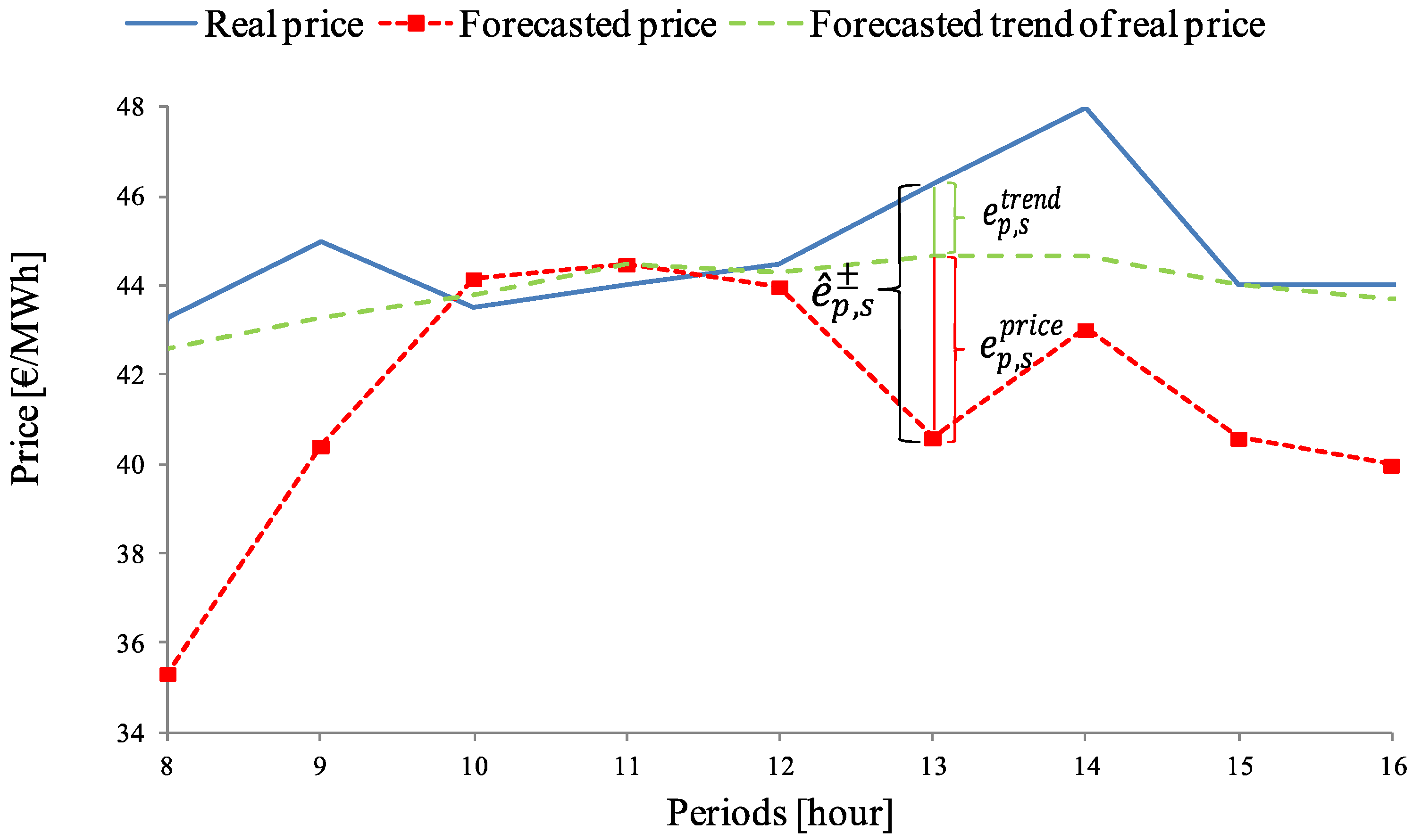
There are three input data, each one being a parameter, namely the forecasted errors ${\widehat{e}}_{p,s}^{forecasts}$, the forecasted trends ${\lambda }_{p,s}$ and the forecasted prices ${\lambda }_{p,s}^{forecasts}$.

The forecasted error (parameter) is an error that corrects the forecasted trends and the forecasted prices, i.e., ${\widehat{e}}_{p,s}^{forecasts}$. This parameter is the possible distance between the real price and the forecasted value. When the real price is lower than the forecasted price, ${\widehat{e}}_{p,s}^{forecasts}$ is negative, and variable ${\widehat{e}}_{p,s}^{-}$ is positive (11), i.e., $z_{p,s}$ binary variable is zero, so ${\widehat{e}}_{p,s}^{\pm }=-{\widehat{e}}_{p,s}^{-}$. The opposite case is $z_{p,s}$ = 1 and ${\widehat{e}}_{p,s}^{\pm }={\widehat{e}}_{p,s}^{+}$, where ${\widehat{e}}_{p,s}^{+}$ is a positive variable, as shown in (10).

The forecasting portfolio is evaluated in (12), where ${\lambda }_{p,s}^{forecasts}$ is the parameter whose values are the forecasts made; one scenario for this parameter is a forecast per period, where variable ${\widehat{\lambda }}_p$ is the final price of the portfolio created by the forecasts, ${\lambda }_{p,s}^{forecasts}$, and the weight that has to be decided, ${\beta }_{p,s}$, whose sum, ${\sum }_s{\beta }_{p,s}$, has to be equal to one, as shown in (13). ${\sum }_s{\beta }_{p,s}$ could be different from one, even being an interval, and the model should decide what is the best value. In this paper, ${\sum }_s{\beta }_{p,s}$ is used as in (13).

Equation (14) decides the value of ${\widehat{\lambda }}_p$ variable; this variable comes from the multiplication of ${\lambda }_{p,s}^{forecasts}$ and the weight ${\beta }_{p,s}$, being ${\widehat{\lambda }}_p$ the final price from (12). Equation (14) reduces the error whose value is the difference between the variable ${\widehat{\lambda }}_p$ and the parameters that are the input data of the model, such as ${\lambda }_{p,s}^{forecasts}$, ${\lambda }_{p,s}$ and ${\widehat{e}}_{p,s}^{\pm }$. The parameter ${\lambda }_{p,s}$ represents the trend of the price; thus, more forecasts provide more information for the possible behavior of the real unknown price. On the other hand, the differences between ${\widehat{\lambda }}_p$ and ${\lambda }_{p,s}$ can be corrected through parameter ${\widehat{e}}_{p,s}^{\pm }$, but also, ${\widehat{e}}_{p,s}^{\pm }$ tries to reduce the imbalance between ${\widehat{\lambda }}_p$ and the real unknown price. Therefore, the forecasting portfolio could improve the ordinary forecasts, but always following parameter ${\lambda }_{p,s}^{forecasts}$.

To sum up, the stochastic programming model is composed of three kinds of input data. These input data are: (i) forecasted prices; (ii) errors of the forecasts that show the differences between the real price (unknown), forecasted price and the trend; and (iii) the trend of the prices (it could be obtained through more forecasts) in order to describe the possible evolution of the price. On the other hand, the variables of the model, $\mathsf{\Theta }=\left\{erro{r}_{p,s},erro{r}_{p,s}^{+},erro{r}_{p,s}^{-},{\widehat{e}}_{p,s}^{\pm },{\widehat{e}}_{p,s}^{+},{\widehat{e}}_{p,s}^{-},{\widehat{\lambda }}_p,{\beta }_{p,s},y_{p,s},z_{p,s}\right\}$, depend on the input data and can be calculated through different techniques.

Index p represents the hour, from Hour 1 spanning the time horizon of forecasting, and index s is the scenario of the stochastic programming model; nevertheless, each s scenario of each input datum can be achieved using any technique to forecast the prices, the error and the trend.

3. Case Study

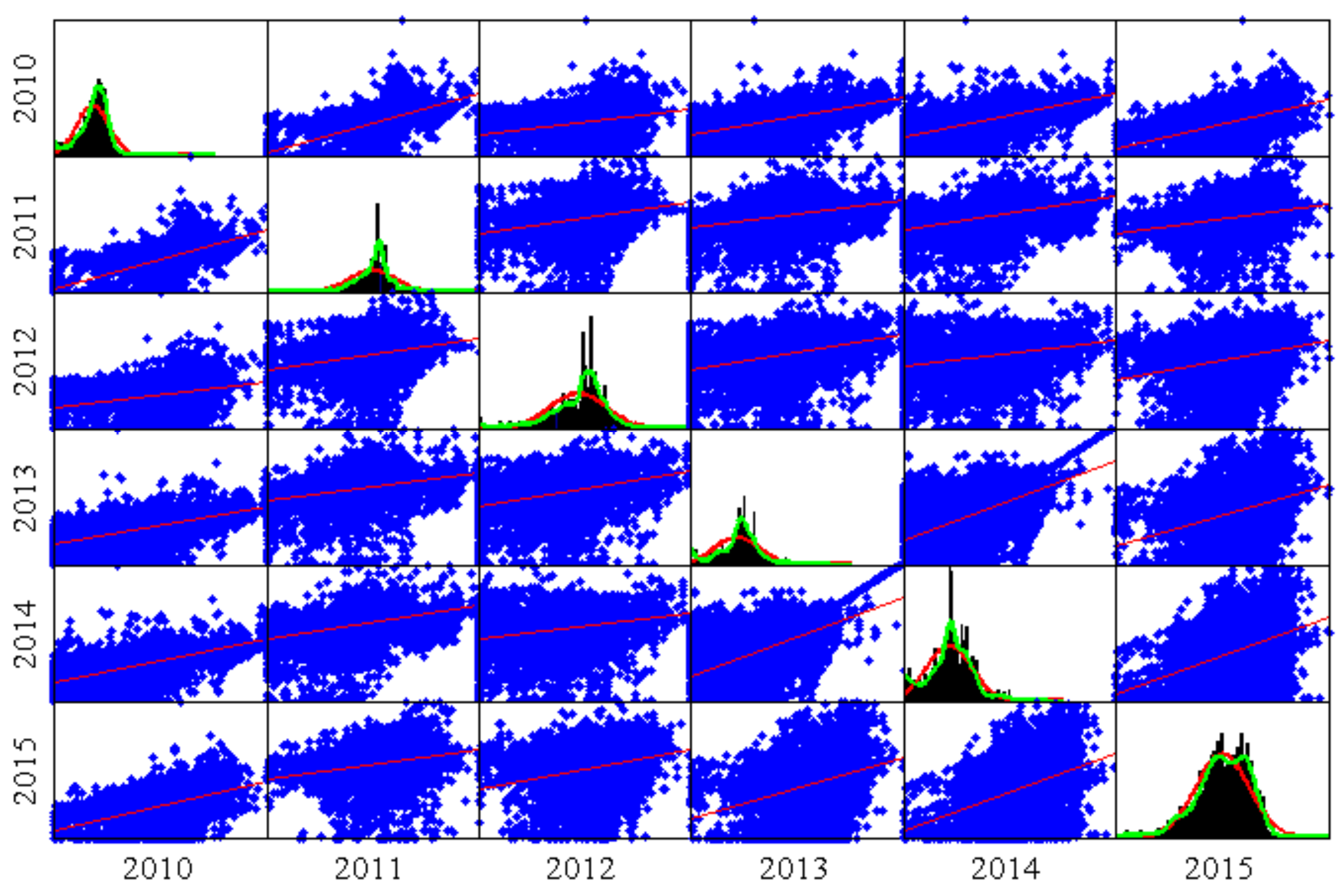
The forecasts are obtained for the Spanish electricity market prices. The prices are quite different for each year;

Table 1. Summary statistics of the Spanish electricity prices (€/MWh) of 2010–2015.

Statistics	2010	2011	2012	2013	2014	2015
Data points	8760	8760	8760	8760	8760	8760
Minimum	0.0	0.0	0.0	0.0	0.0	4.0
10% percentile	15.13	38.57	30.49	10.0	10.0	33.99
25% percentile	30.08	45.93	40.77	34.00	30.50	43.10
Mean	37.00	49.92	47.21	44.26	43.09	50.32
Geometric mean	-	-	-	-	-	48.24
Harmonic mean	10.85	24.70	13.99	4.86	6.48	44.54
Median	40.00	52.00	50.00	47.00	44.83	51.20
75% percentile	46.41	55.23	55.0	55.96	56.17	60.00
90% percentile	51.50	60.18	60.12	65.13	67.16	64.88
Maximum	145.00	91.01	90.13	112.00	113.92	85.05
Interquartile range	16.33	9.29	14.23	21.96	25.67	16.90
Range	36.37	21.60	29.63	55.13	57.16	30.89
Standard deviation	14.69	10.60	13.13	20.73	21.14	12.37
Variance	216.02	112.45	172.64	429.99	447.00	153.03
Mean absolute deviation	11.10	7.17	9.86	15.44	16.17	9.81
Median absolute deviation	7.77	3.99	6.52	10.32	12.34	8.50
Mean/Standard deviation	2.51	4.70	3.59	2.13	2.03	4.06
Skewness	−0.60	−1.33	−1.18	−0.29	−0.07	−0.71
Kurtosis	1.18	4.86	1.98	0.45	0.12	0.64

shows a summary of the statistics, and

Table 2. Correlation matrix of the Spanish electricity prices of 2010–2015.

Years	2010	2011	2012	2013	2014	2015
2010	1	0.49	0.26	0.50	0.57	0.53
2011	0.49	1	0.30	0.31	0.40	0.28
2012	0.26	0.30	1	0.33	0.25	0.31
2013	0.50	0.31	0.33	1	0.58	0.37
2014	0.57	0.40	0.25	0.58	1	0.46
2015	0.53	0.28	0.31	0.37	0.46	1

presents the correlation matrix of the Spanish electricity prices from 2010–2015 [33]. The high standard deviation of prices of years 2013 and 2014 is remarkable, whose values are €20.73/MWh and €21.14/MWh, respectively. These values are two-times the standard deviation of the prices of 2011. This analysis is made using ECOTOOL (2016) [34], a forecasting toolbox in MATLAB^® (R2011b) [35].

Figure 1 portrays the scatter plots and the histograms of all of the hourly prices of each one of the six years. Red lines in the histograms indicate the shape of the normal distribution, whilst the green lines describe the real shape of the distribution that follows those data. Figure 2 depicts the sample of 2016, from 1 January–10 June 2016; the mean price is equal to €29.17/MWh, and the standard deviation of prices is €12.35/MWh. The time series of the day-ahead electricity market prices is transformed using a logarithmic transformation to make the dispersion constant.

3.1. Input Data for the SP Model

As presented in Section 2, there are three input data: forecasted prices, forecasted errors and forecasted trends. This section shows how these input data are calculated to test the SP model, achieving a portfolio of the forecasted prices, which are input data.

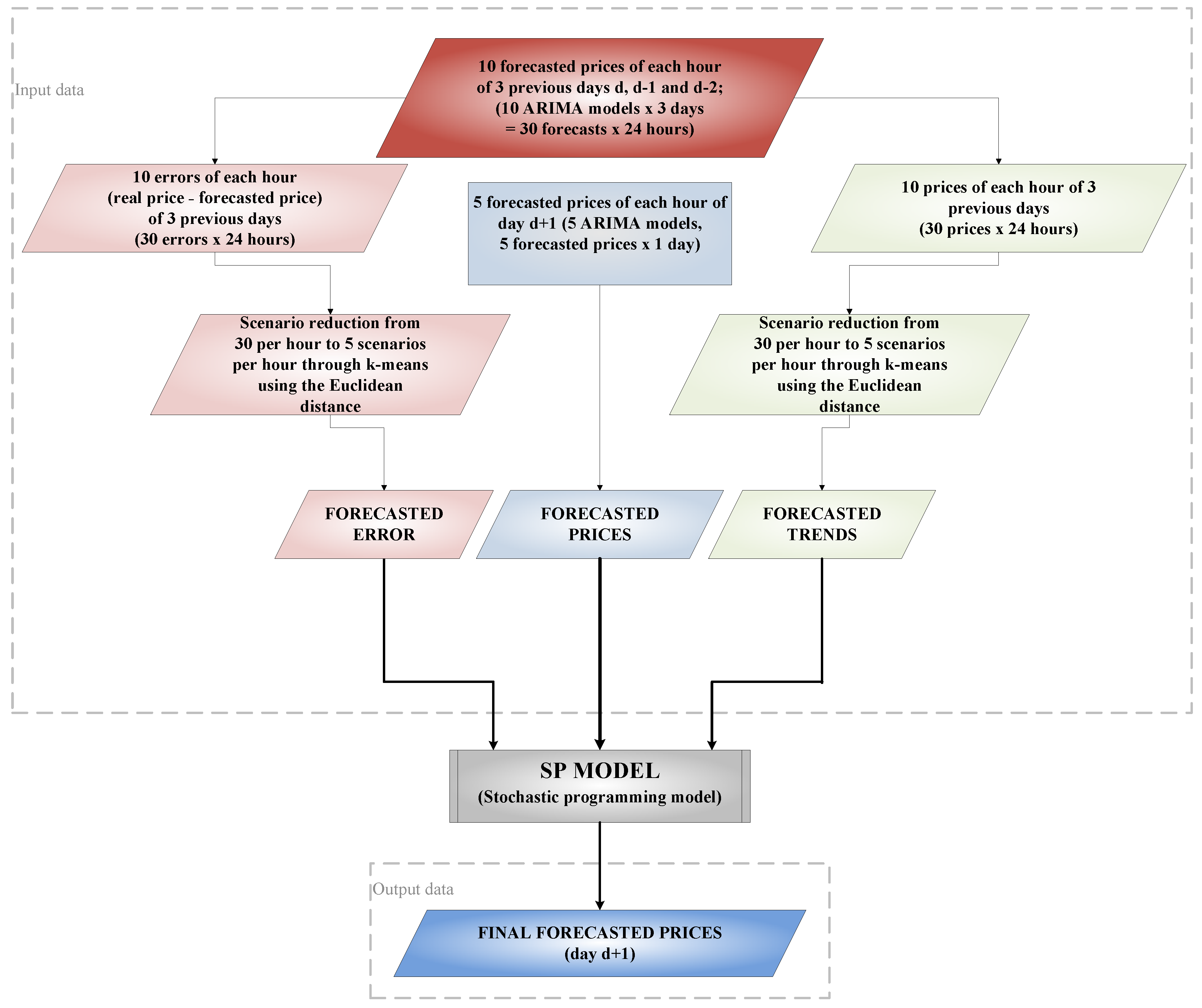
Figure 3 shows the three input data: forecasted prices, forecasted errors and forecasted trends; all of them represent the information used in the SP model. Moreover, Figure 3 shows the main output data, i.e., the final forecasted prices.

Figure 3 presents how the different inputs are calculated. There are two forecasting processes; first, some forecasts are made for the three days (d, $d-1$, and $d-2$) previous to the final day ($d+1$) in order to have more information; and second, some forecasts are made only for the final day ($d+1$).

The first forecasting process is used to determine the behavior of the errors and trends of the three days previous to day $d+1$, where the models are similar to the models used in the second forecasting process. The three previous days are utilized because the real prices of these days are known; thus, the behavior of the errors and trends can be calculated from these forecasts. Thirty scenarios of trends and errors are attained for each hour of the day, 3 days × 10 models × 24 h. The 30 scenarios per hour are reduced to five scenarios per hour for the errors and trends. The scenario reduction from 30 scenarios per hour to five scenarios per hour is done by the k-means method using the Euclidean distance, where the centroid is the mean of the points of the cluster of the five scenarios.

The second forecasting process is applied to day $d+1$, that is the real forecasted day, and five forecasted prices are obtained from the first five ARIMA models of

Table 3. Terms of the ARIMA models.

Model	Seasonal Parameters $(1-{\mathit{B}}_{\mathit{j}}^{\mathit{s}})$	AR Parameters ${\mathit{\varphi }}_{{\mathit{p}}_{\mathit{j}}}({\mathit{B}}^{{\mathit{s}}_{\mathit{j}}})$	MA Parameters ${\mathit{\theta }}_{{\mathit{q}}_{\mathit{j}}}({\mathit{B}}^{{\mathit{s}}_{\mathit{j}}})$
ARIMA1	1, 24	1, 2, 24	2, 24
ARIMA2	1, 24	1, 2, 7, 24	1, 2
ARIMA3	-	1, 2, 7, 9, 24	2
ARIMA4	-	1, 2, 7, 19, 24, 27	1
ARIMA5	-	1, 2, 3, 7, 19, 21, 24	1, 2
ARIMA6	-	1, 2, 3, 7, 9, 24, 27, 48	2
ARIMA7	-	1, 2, 3, 7, 19, 21, 24	1, 2
ARIMA8	1, 24	1, 24, 168	1
ARIMA9	1, 24	1, 2, 24, 168	1
ARIMA10	1, 24	1, 24, 168	2

. Five ARIMA models are used because the stochastic programming model presented in Section 2 is tested utilizing five scenarios.

Note that the forecasting processes previous to the SP model can be done by means of neural networks, support vector machines, ensemble methods or by a mixture of all of them, with the possibility of including other methods.

The information of the input data comes from the use of ARIMA models. The behavior of previous days for each forecast is used in order to obtain the forecasted error and the forecasted trend.

3.2. ARIMA Models

The proposed general ARIMA formulation [34] is as follows:

$$\begin{array}{lll}{y}_t& =& c+\frac{1}{{(1-B)}^{d_0}{(1-B^{s_1})}^{d_1}\dots {(1-B^{s_k})}^{d_k}}\\ & & \times \frac{{\theta }_{q_0}\left(B\right)}{{\varphi }_{p_0}\left(B\right)}\frac{{\theta }_{q_1}\left(B^{s_1}\right)}{{\varphi }_{p_1}\left(B^{s_1}\right)}\times \dots \times \frac{{\theta }_{q_k}\left(B^{s_k}\right)}{{\varphi }_{p_k}\left(B^{s_k}\right)}{ϵ}_t.\end{array}$$

(16)

where $y_t$ is the observed time series, ${ϵ}_t$ is the residual term, $s_j$, $j=0,\dots ,k$ is a set of seasonal periods, $s_0=1$, $(1-B_j^s)$, $j=0,1,\dots ,k$ are the $k+1$ differencing operators necessary to reduce the time series and to achieve mean stationary, ${\varphi }_{p_j}\left(B^{s_j}\right)$ and ${\theta }_{q_j}\left(B^{s_j}\right)$, $j=0,1,\dots ,k$ are the AR and MA polynomials of the back shift operator B: $B^l{y}_t=y_{t-l}$ of ${\theta }_{q_j}\left(B^{s_j}\right)=(1+{\theta }_1{B}^{s_j}+{\theta }_2{B}^{2s_j}+\dots +{\theta }_j{B}^{q_j{s}_j})$, and c is a constant.

Previously, the time series is transformed through logarithmic transformation to stabilize the variance; after that, ARIMA models can be applied.

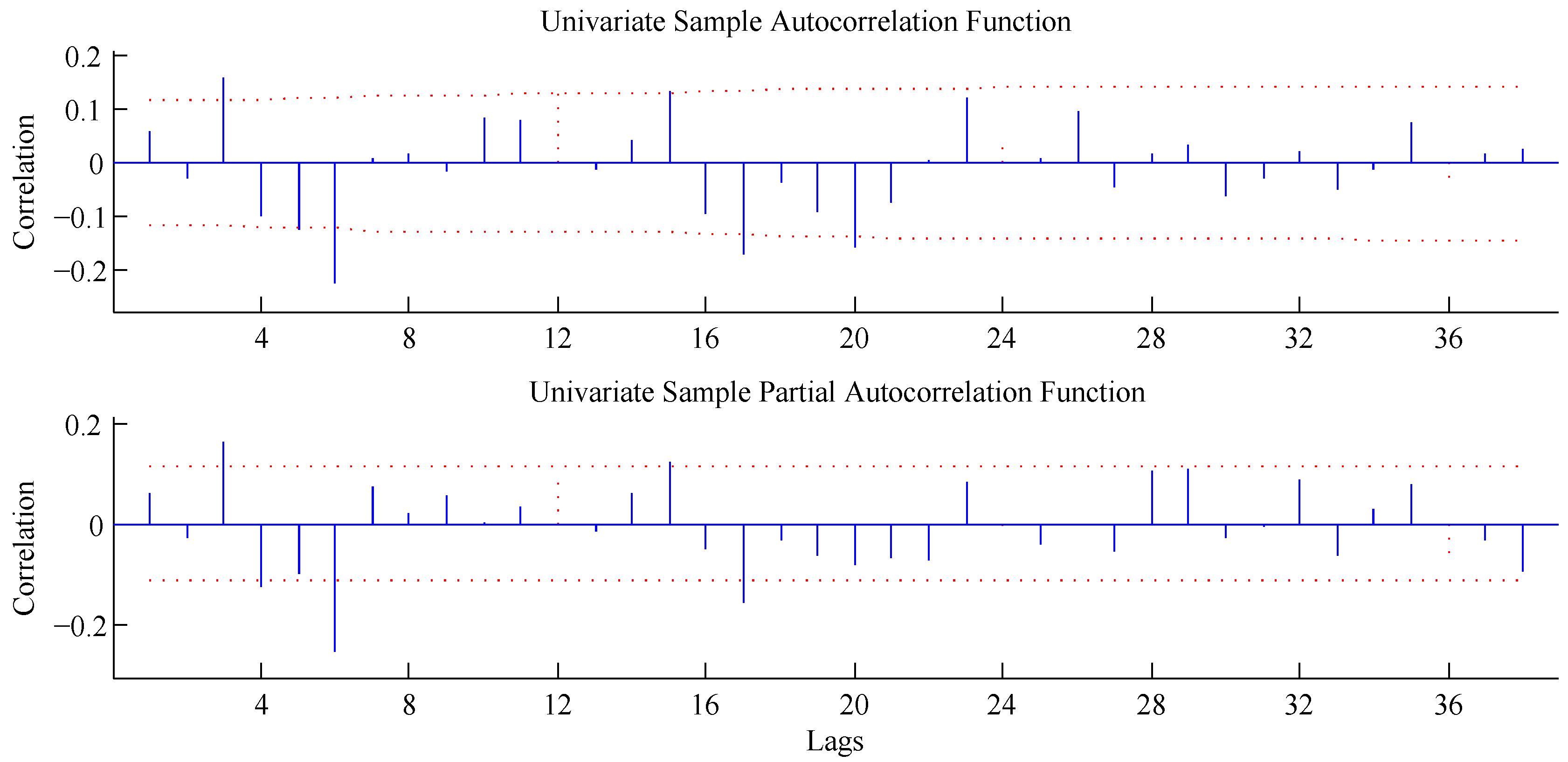
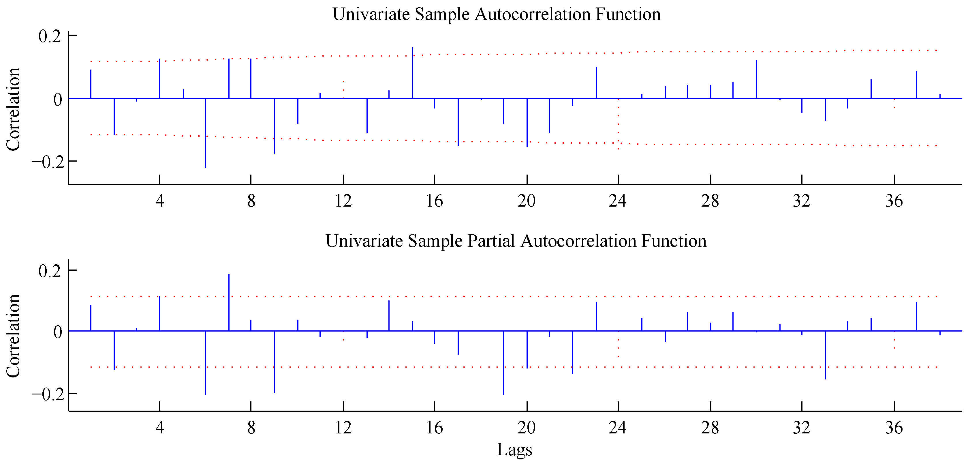
Following the formulation of (16), the indexes of each term for every ARIMA model are shown in Table 3. The process to select each term of each ARIMA model is based on the evaluation of each autocorrelation function (ACF) and partial autocorrelation function (PACF) of the residual component, ${ϵ}_t$, of each ARIMA model, as shown in Figure 4 and Figure 5.

Figure 4 and Figure 5 portray the ACF and PACF of the residual terms for the ARIMA 2 model for 5 and 6 June 2016. The ARIMA model formulation of the ARIMA 2 model is presented in (17), where it is easy to identify every term.

$$\begin{array}{c}{y}_t=c+\frac{1}{(1-B)(1-B^{24})}\frac{(1-{\theta }_{1}B-{\theta }_2{B}^2)}{(1-{\varphi }_{1}B-{\varphi }_2{B}^2-{\varphi }_7{B}^7)}\frac{1}{(1-{\varphi }_{24}{B}^{24})}{ϵ}_t.\hfill \end{array}$$

(17)

3.3. Forecasted Prices

Forecasted prices are obtained through ARIMA models; this case study uses five scenarios. These five scenarios for the input data of forecasted prices are ARIMA 1, ARIMA 2, ARIMA 3, ARIMA 4 and ARIMA 5, as presented in Table 3, where each ARIMA model represents one scenario. An econometric toolbox of MATLAB^® [35], ECOTOOL [34], is used to obtain the forecasts. The sample used to forecast every day with each ARIMA model is 15 days, i.e., 360 h. A sample spanning 360 h has been selected because the sample changes every two or three weeks as a consequence of the price volatility. The computing time increases for a sample spanning more days.

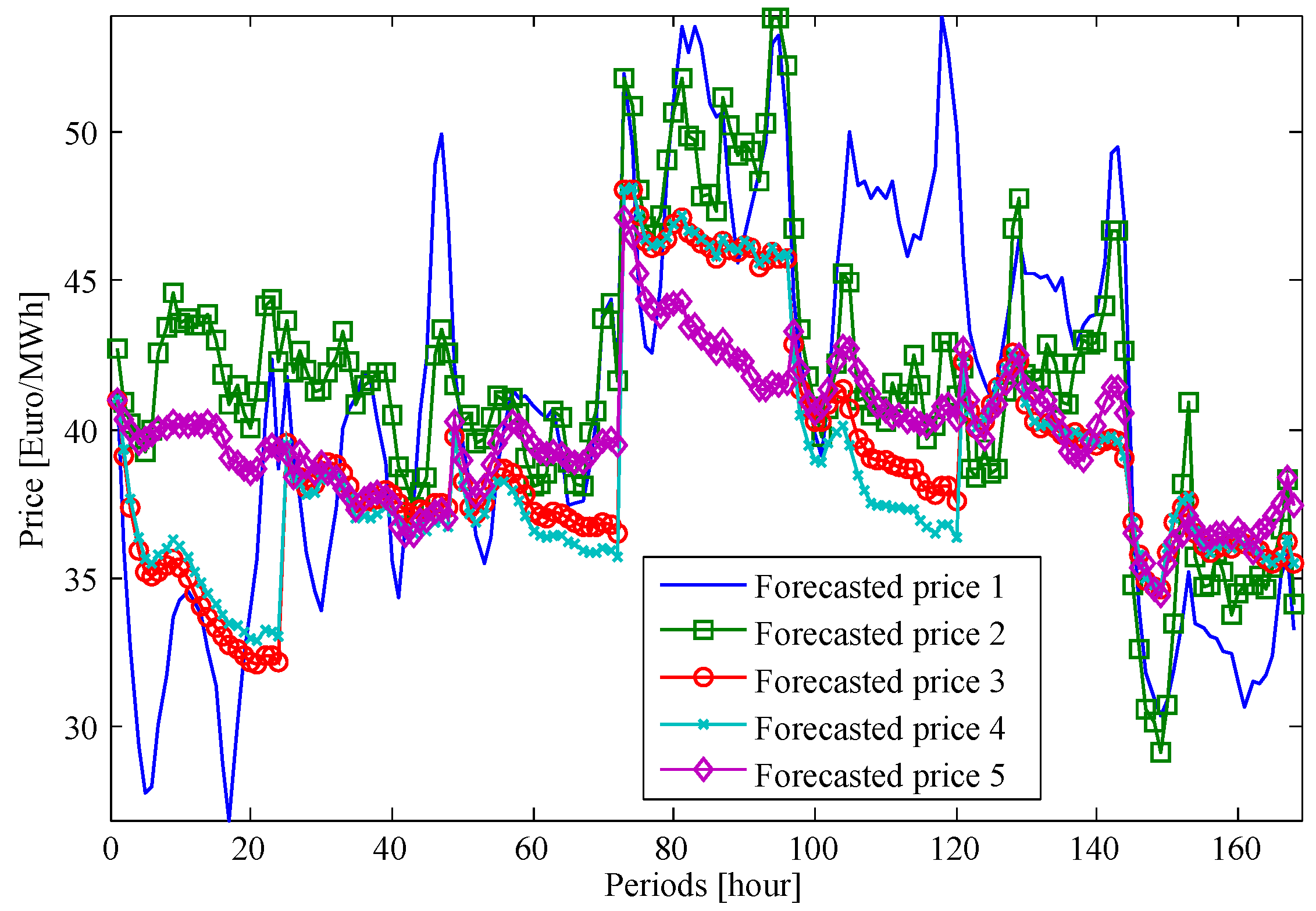
The five scenarios of forecasted prices are depicted in Figure 6, where one week of forecasts is shown. The forecasted days span from the 4–10 June 2016. After this, the models are verified for one week of each season of 2014, 2015 and 2016, the forecasting horizon being 24 h using a 24-h rolling horizon window for the next day until every day of each week is evaluated.

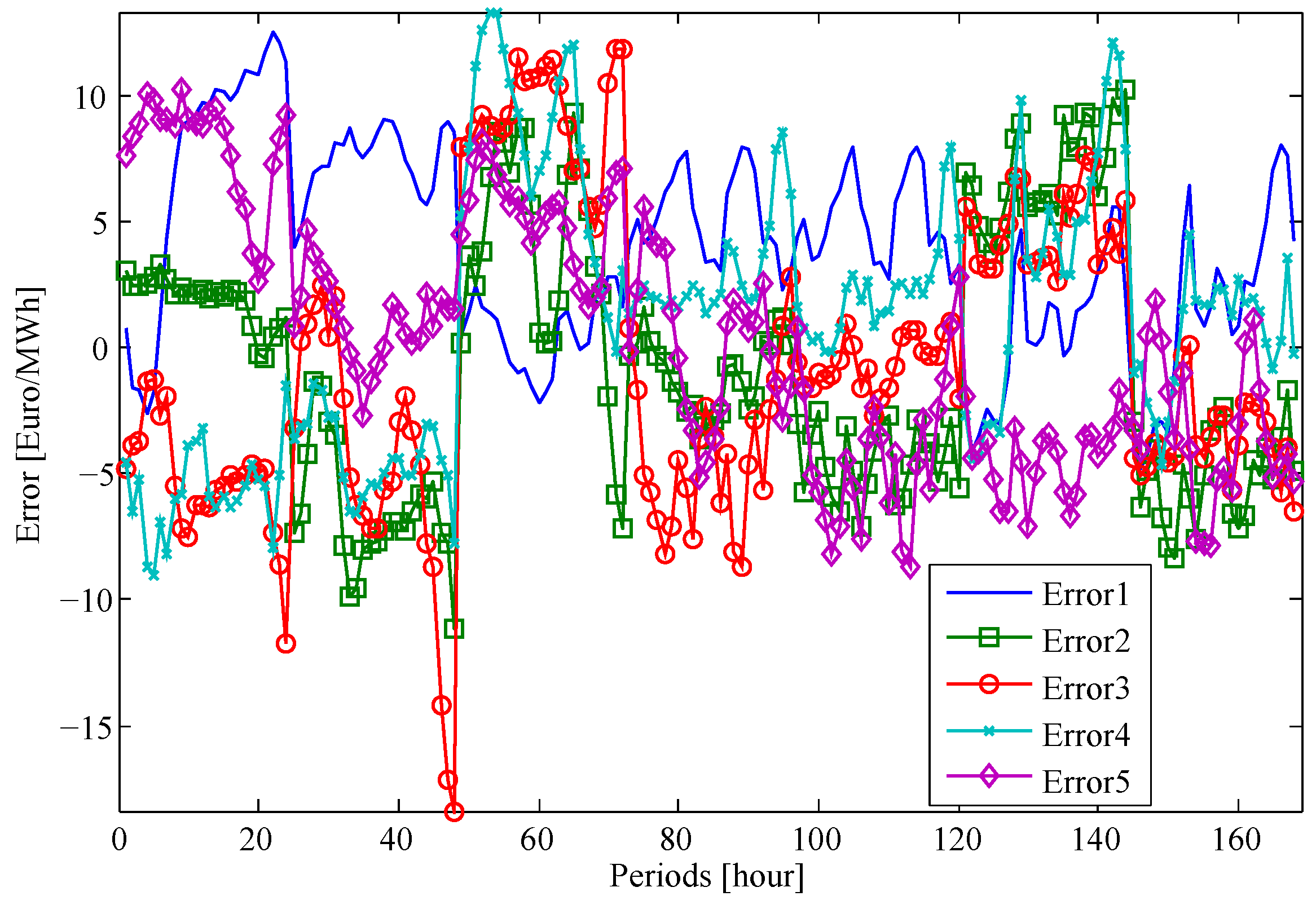
3.4. Forecasted Errors

Errors are the differences between the real price and the forecasted price, being positive when the real price is higher than the forecasted price and negative otherwise. It is remarkable that, if for the forecasting day the real price are unknown, then the error is also unknown. However, the error can be calculated for previous days since the real price is known. Thus, the ten ARIMA models of Table 3 are used to make forecasts of the three previous days. As a consequence of using 10 ARIMA models in these three days, the number of scenarios of forecasted errors would be 30 (10 ARIMA models multiplied by three days), but they can be reduced to five scenarios. Scenario reduction is performed through the squared Euclidean distance, and each centroid is the mean of the points in the cluster for five scenarios, reducing them from 30 down to five. The input data forecasted errors are these five scenarios.

The five scenarios obtained from the 30 scenarios are shown in Figure 7.

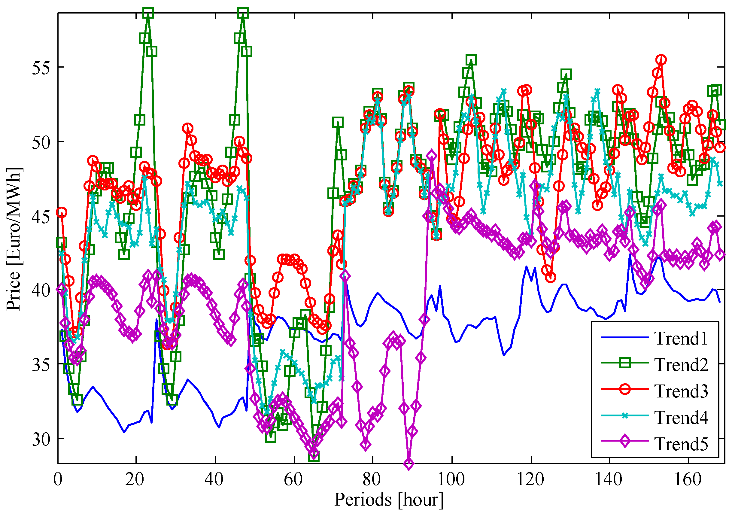
3.5. Forecasted Trends

Forecasted trends are made through the 10 ARIMA models of Table 3. The forecasted trend is made for the three previous days, trying to recover some behaviors of previous days. Therefore, as happened for the forecasted error input data, the forecasted trend has 30 scenarios, three days multiplied by 10 forecasts of the 10 ARIMA models. The scenarios are reduced through the squared Euclidean distance as done for the forecasted error. The five scenarios of forecasted trends are depicted in Figure 8.

4. Results and Discussion

4.1. Results

This subsection shows the results obtained using this technique for the forecasting week. Firstly, the daily average errors (%) ($DAE$) of the week under study are calculated in (18), where $p_t$ is the real price, ${\widehat{p}}_t$ is the forecasted price and $\overline{p}$ is the average real price of the 24 hours. Secondly, the errors (18) from 1–10 June 2016 are presented in

Table 4. Daily average error (%) of 1–10 June 2016, for ARIMA Models 1–10.

Model/Day of June (%)	1	2	3	4	5	6	7	8	9	10
ARIMA 1	5.56	14.16	23.33	16.09	6.24	10.49	8.03	9.47	8.03	18.08
ARIMA 2	13.05	16.33	11.42	7.28	5.55	9.31	8.31	8.28	4.54	13.74
ARIMA 3	20.22	21.67	21.17	13.16	4.61	15.48	3.35	12.01	7.73	10.48
ARIMA 4	21.38	22.17	21.15	11.56	5.72	16.81	3.43	13.58	7.65	10.39
ARIMA 5	20.01	20.11	23.97	3.10	5.04	11.53	6.36	8.98	6.94	9.92
ARIMA 6	21.55	7.56	15.50	8.43	7.78	15.59	5.11	12.76	6.26	9.43
ARIMA 7	20.01	20.11	23.97	3.10	5.04	11.53	6.36	8.98	6.94	9.92
ARIMA 8	16.34	11.93	15.56	6.38	12.25	10.71	11.15	6.37	4.40	9.13
ARIMA 9	15.73	12.91	15.87	6.38	12.42	10.33	10.60	6.42	6.23	8.68
ARIMA 10	16.08	12.82	15.78	6.27	11.87	9.97	11.45	6.40	4.46	9.09

. Several input data are calculated through the forecasts of the three previous days, and due to that, Days 1, 2 and 3 of June are presented in Table 4, as well.

$$\begin{array}{c}DAE(\%)=e_{day}(\%)=\frac{1}{24}\sum _{t=1}^{24}\frac{\left|p_t-{\widehat{p}}_t\right|}{\overline{p}}·100.\hfill \end{array}$$

(18)

$DAE$ for the SP model of

Table 5. Daily average error (%) of 4–10 June 2016, for the SP model, average, and ARIMA Models 1–5.

Model/Day of June (%)	4	5	6	7	8	9	10
SP	7.36	2.91	11.93	2.99	7.55	7.84	9.16
Average	7.17	3.15	12.73	3.36	7.92	5.57	12.19
ARIMA 1	16.09	6.24	10.49	8.03	9.47	8.03	18.08
ARIMA 2	7.28	5.55	9.31	8.31	8.28	4.54	13.74
ARIMA 3	13.16	4.61	15.48	3.35	12.01	7.73	10.48
ARIMA 4	11.56	5.72	16.81	3.43	13.58	7.65	10.39
ARIMA 5	3.10	5.04	11.53	6.36	8.98	6.94	9.92

Note that the numbers in bold indicate that the SP model has the lowest error compared to the average model.

can be lower and higher than the average price forecasting (AVG), but this depends on the forecasted errors and trends used as input data, where the final error is lower when the forecasted trend and forecasted error follow the forecasted price. The differences between forecasted price, trend and error can increase or reduce the final error.

The forecasted week of June of 2016 is portrayed in Figure 9, and

Table 6. $\beta \in [0,1]$ values in each scenario of the forecasted price for the second and third days of the week.

Hour/Scenario	1	2	3	4	5	Hour/Scenario	1	2	3	4	5
25	0.94	0.06	0	0	0	49	0.53	0	0	0.47	0
26	0.60	0.40	0	0	0	50	0.04	0.96	0	0	0
27	0.53	0.47	0	0	0	51	0.21	0.79	0	0	0
28	0.65	0.35	0	0	0	52	0.16	0.84	0	0	0
29	0.35	0.65	0	0	0	53	0.24	0.76	0	0	0
30	0.28	0.72	0	0	0	54	0.43	0.57	0	0	0
31	0.27	0.73	0	0	0	55	0.81	0.19	0	0	0
32	0.37	0.63	0	0	0	56	0.28	0	0	0.72	0
33	0.82	0.18	0	0	0	57	0.49	0	0	0.51	0
34	0	0.54	0	0.46	0	58	0.70	0	0	0.30	0
35	0.73	0	0	0.27	0	59	0.78	0	0	0.22	0
36	0.70	0	0	0.30	0	60	0.26	0	0	0.74	0
37	0.75	0	0	0.25	0	61	0.38	0	0	0.62	0
38	0.62	0.38	0	0	0	62	0.41	0	0	0.59	0
39	0.36	0.64	0	0	0	63	0.90	0	0	0.10	0
40	0.15	0.85	0	0	0	64	0.32	0.68	0	0	0
41	0	0.75	0	0	0.25	65	0	0	0	0.28	0.72
42	0	1.00	0	0	0	66	0.89	0	0	0	0.11
43	1.00	0	0	0	0	67	1.00	0	0	0	0
44	0.80	0	0	0.20	0	68	0.93	0	0	0.07	0
45	0.47	0	0	0.53	0	69	0.59	0	0	0.41	0
46	0.40	0	0	0.60	0	70	0.51	0	0	0.49	0
47	0	0.76	0	0.24	0	71	0	0.46	0	0.54	0
48	0.35	0	0	0.65	0	72	0.44	0	0	0.56	0

shows the weight of each forecasted price, ${\lambda }_{p,s}^{forecasts}$, introduced in the SP model for the second and third forecasted days, the best and worst forecasted day of the SP model, respectively.

For this case study, ${\beta }_{p,s}\in [0,1]$, but this value could be different allowing for an increase or a decrease in the forecasted price weight. The main dissimilarity between ${\beta }_{p,s}$ of Table 6 is for the best day; the percentage of each forecasted price of the input data is more distributed between two scenarios of the input data.

After showing one week for the spring season of the current year, 2016, and in order to evaluate the forecasts per season,

Table 7. $e_{day}$ (%), $e_{FMSE}^{day}$ and ${\sigma }_{e,day}^2$ of winter of 2016, 2015 and 2014 for the SP model, average (AVG) and naïve models.

Winter (January 2016)
Day	SP			AVG			Naïve
	${\mathit{e}}_{\mathit{day}}$ %	${\mathit{e}}_{\mathit{FMSE}}^{\mathit{day}}$	${\mathit{\sigma }}_{\mathit{e},\mathit{day}}^{\mathbf{2}}$	${\mathit{e}}_{\mathit{day}}$ %	${\mathit{e}}_{\mathit{FMSE}}^{\mathit{day}}$	${\mathit{\sigma }}_{\mathit{e},\mathit{day}}^{\mathbf{2}}$	${\mathit{e}}_{\mathit{day}}$ %	${\mathit{e}}_{\mathit{FMSE}}^{\mathit{day}}$	${\mathit{\sigma }}_{\mathit{e},\mathit{day}}^{\mathbf{2}}$
Saturday	19.03	7.95	0.0151	10.52	4.84	0.0080	22.24	10.74	0.0441
Sunday	13.44	6.16	0.0093	18.29	7.99	0.0126	68.60	25.78	0.0083
Monday	16.34	8.04	0.0093	20.31	9.90	0.0133	39.30	18.26	0.0311
Tuesday	20.34	11.97	0.0116	32.87	19.48	0.0322	18.82	11.18	0.0108
Wednesday	15.11	9.17	0.0071	23.33	14.45	0.0197	3.58	2.61	0.0012
Thursday	17.29	10.23	0.0102	9.67	5.95	0.0042	7.04	4.61	0.0032
Friday	6.67	3.94	0.0025	16.92	9.22	0.0095	10.38	5.69	0.0038
Winter (January 2015)
Day	SP			AVG			Naïve
	${\mathit{e}}_{\mathit{day}}$ %	${\mathit{e}}_{\mathit{FMSE}}^{\mathit{day}}$	${\mathit{\sigma }}_{\mathit{e},\mathit{day}}^{\mathbf{2}}$	${\mathit{e}}_{\mathit{day}}$ %	${\mathit{e}}_{\mathit{FMSE}}^{\mathit{day}}$	${\mathit{\sigma }}_{\mathit{e},\mathit{day}}^{\mathbf{2}}$	${\mathit{e}}_{\mathit{day}}$ %	${\mathit{e}}_{\mathit{FMSE}}^{\mathit{day}}$	${\mathit{\sigma }}_{\mathit{e},\mathit{day}}^{\mathbf{2}}$
Saturday	8.85	5.60	0.0066	11.95	6.56	0.0056	21.75	11.28	0.0113
Sunday	14.60	8.02	0.0138	13.97	7.30	0.0096	18.06	8.78	0.0095
Monday	11.31	7.32	0.0069	22.39	13.66	0.0185	14.64	8.58	0.0056
Tuesday	10.31	7.87	0.0062	10.42	6.93	0.0023	13.87	9.73	0.0066
Wednesday	12.78	9.14	0.0144	14.38	9.95	0.0158	20.94	12.79	0.0164
Thursday	9.58	5.66	0.0033	12.53	7.34	0.0053	15.12	8.93	0.0082
Friday	4.40	3.14	0.0015	6.64	4.13	0.0015	6.36	4.46	0.0029
Winter (January 2014)
Day	SP			AVG			Naïve
	${\mathit{e}}_{\mathit{day}}$ %	${\mathit{e}}_{\mathit{FMSE}}^{\mathit{day}}$	${\mathit{\sigma }}_{\mathit{e},\mathit{day}}^{\mathbf{2}}$	${\mathit{e}}_{\mathit{day}}$ %	${\mathit{e}}_{\mathit{FMSE}}^{\mathit{day}}$	${\mathit{\sigma }}_{\mathit{e},\mathit{day}}^{\mathbf{2}}$	${\mathit{e}}_{\mathit{day}}$ %	${\mathit{e}}_{\mathit{FMSE}}^{\mathit{day}}$	${\mathit{\sigma }}_{\mathit{e},\mathit{day}}^{\mathbf{2}}$
Saturday	19.65	10.94	0.0087	13.69	9.38	0.0161	90.07	46.07	0.0286
Sunday	27.86	11.92	0.0227	9.04	4.77	0.0079	89.13	33.98	0.0193
Monday	22.83	11.08	0.0294	23.16	11.68	0.0370	72.07	31.79	0.1515
Tuesday	43.30	16.27	0.0225	45.91	18.26	0.0536	45.27	18.13	0.0906
Wednesday	25.24	14.41	0.0199	21.99	12.16	0.0112	34.03	20.63	0.0555
Thursday	14.90	7.08	0.0066	18.42	9.00	0.0125	21.29	10.14	0.0136
Friday	24.22	11.33	0.0189	46.91	21.30	0.0539	11.94	7.05	0.0157

,

Table 8. $e_{day}$ (%), $e_{FMSE}^{day}$ and ${\sigma }_{e,day}^2$ of spring of 2016, 2015 and 2014 for the SP model, average and naïve models.

Spring (June, 2016)
Day	SP			AVG			Naïve
	${\mathit{e}}_{\mathit{day}}$ %	${\mathit{e}}_{\mathit{FMSE}}^{\mathit{day}}$	${\mathit{\sigma }}_{\mathit{e},\mathit{day}}^{\mathbf{2}}$	${\mathit{e}}_{\mathit{day}}$ %	${\mathit{e}}_{\mathit{FMSE}}^{\mathit{day}}$	${\mathit{\sigma }}_{\mathit{e},\mathit{day}}^{\mathbf{2}}$	${\mathit{e}}_{\mathit{day}}$ %	${\mathit{e}}_{\mathit{FMSE}}^{\mathit{day}}$	${\mathit{\sigma }}_{\mathit{e},\mathit{day}}^{\mathbf{2}}$
Saturday	7.36	3.30	0.0015	7.17	3.18	0.0013	40.20	16.30	0.0068
Sunday	2.91	1.57	0.0007	3.14	1.68	0.0008	68.09	27.73	0.0232
Monday	11.93	5.63	0.0019	12.72	5.85	0.0012	20.39	9.73	0.0065
Tuesday	2.99	1.67	0.0004	3.36	1.77	0.0003	3.86	2.06	0.0005
Wednesday	7.55	3.75	0.0021	7.92	4.00	0.0026	9.01	4.73	0.0043
Thursday	7.84	3.93	0.0028	5.56	2.73	0.0012	5.05	2.90	0.0024
Friday	9.16	4.75	0.0057	12.18	5.82	0.0063	7.93	3.85	0.0030
Spring (June, 2015)
Day	SP			AVG			Naïve
	${\mathit{e}}_{\mathit{day}}$ %	${\mathit{e}}_{\mathit{FMSE}}^{\mathit{day}}$	${\mathit{\sigma }}_{\mathit{e},\mathit{day}}^{\mathbf{2}}$	${\mathit{e}}_{\mathit{day}}$ %	${\mathit{e}}_{\mathit{FMSE}}^{\mathit{day}}$	${\mathit{\sigma }}_{\mathit{e},\mathit{day}}^{\mathbf{2}}$	${\mathit{e}}_{\mathit{day}}$ %	${\mathit{e}}_{\mathit{FMSE}}^{\mathit{day}}$	${\mathit{\sigma }}_{\mathit{e},\mathit{day}}^{\mathbf{2}}$
Saturday	12.78	7.72	0.0091	10.62	6.47	0.0066	8.86	5.15	0.0035
Sunday	9.98	5.95	0.0067	11.51	6.62	0.0074	7.64	4.09	0.0020
Monday	8.92	5.81	0.0028	11.35	7.20	0.0037	1.66	1.37	0.0003
Tuesday	10.00	6.57	0.0032	6.58	4.00	0.0005	2.42	1.78	0.0003
Wednesday	3.13	2.25	0.0005	4.45	3.44	0.0016	5.35	3.81	0.0016
Thursday	5.38	3.59	0.0005	5.17	3.52	0.0006	6.04	4.05	0.0008
Friday	3.52	2.75	0.0009	5.92	4.25	0.0018	5.71	3.89	0.0012
Spring (June 2014)
Day	SP			AVG			Naïve
	${\mathit{e}}_{\mathit{day}}$ %	${\mathit{e}}_{\mathit{FMSE}}^{\mathit{day}}$	${\mathit{\sigma }}_{\mathit{e},\mathit{day}}^{\mathbf{2}}$	${\mathit{e}}_{\mathit{day}}$ %	${\mathit{e}}_{\mathit{FMSE}}^{\mathit{day}}$	${\mathit{\sigma }}_{\mathit{e},\mathit{day}}^{\mathbf{2}}$	${\mathit{e}}_{\mathit{day}}$ %	${\mathit{e}}_{\mathit{FMSE}}^{\mathit{day}}$	${\mathit{\sigma }}_{\mathit{e},\mathit{day}}^{\mathbf{2}}$
Saturday	15.33	10.34	0.0115	10.88	7.03	0.0044	25.18	14.90	0.0093
Sunday	7.26	4.66	0.0030	8.40	5.04	0.0026	61.46	31.95	0.0123
Monday	14.12	10.28	0.0064	18.05	12.79	0.0081	35.02	24.02	0.0210
Tuesday	3.49	3.03	0.0009	5.77	3.86	0.0002	4.20	4.10	0.0023
Wednesday	11.86	8.77	0.0102	10.82	7.57	0.0063	15.56	11.41	0.0169
Thursday	2.68	2.05	0.0004	7.13	4.60	0.0007	6.76	5.41	0.0035
Friday	7.06	5.57	0.0029	5.84	4.12	0.0008	7.77	6.51	0.0047

,

Table 9. $e_{day}$ (%), $e_{FMSE}^{day}$ and ${\sigma }_{e,day}^2$ of summer of 2016, 2015 and 2014 for the SP model, average and naïve models.

Summer (August 2016)
Day	SP			AVG			Naïve
	${\mathit{e}}_{\mathit{day}}$ %	${\mathit{e}}_{\mathit{FMSE}}^{\mathit{day}}$	${\mathit{\sigma }}_{\mathit{e},\mathit{day}}^{\mathbf{2}}$	${\mathit{e}}_{\mathit{day}}$ %	${\mathit{e}}_{\mathit{FMSE}}^{\mathit{day}}$	${\mathit{\sigma }}_{\mathit{e},\mathit{day}}^{\mathbf{2}}$	${\mathit{e}}_{\mathit{day}}$ %	${\mathit{e}}_{\mathit{FMSE}}^{\mathit{day}}$	${\mathit{\sigma }}_{\mathit{e},\mathit{day}}^{\mathbf{2}}$
Saturday	12.74	6.17	0.0060	7.56	3.74	0.0024	11.98	5.40	0.0026
Sunday	8.99	4.18	0.0035	16.09	7.08	0.0073	15.70	6.46	0.0030
Monday	4.52	2.13	0.0006	4.69	2.32	0.0009	9.22	4.12	0.0015
Tuesday	9.19	5.20	0.0050	7.09	4.17	0.0036	9.20	5.63	0.0073
Wednesday	3.17	1.60	0.0003	2.12	1.32	0.0004	3.87	2.37	0.0015
Thursday	4.02	2.01	0.0005	4.27	2.11	0.0005	3.53	1.88	0.0006
Friday	3.45	1.78	0.0005	3.88	1.90	0.0005	4.64	2.39	0.0011
Summer (August 2015)
Day	SP			AVG			Naïve
	${\mathit{e}}_{\mathit{day}}$ %	${\mathit{e}}_{\mathit{FMSE}}^{\mathit{day}}$	${\mathit{\sigma }}_{\mathit{e},\mathit{day}}^{\mathbf{2}}$	${\mathit{e}}_{\mathit{day}}$ %	${\mathit{e}}_{\mathit{FMSE}}^{\mathit{day}}$	${\mathit{\sigma }}_{\mathit{e},\mathit{day}}^{\mathbf{2}}$	${\mathit{e}}_{\mathit{day}}$ %	${\mathit{e}}_{\mathit{FMSE}}^{\mathit{day}}$	${\mathit{\sigma }}_{\mathit{e},\mathit{day}}^{\mathbf{2}}$
Saturday	6.97	5.48	0.0051	7.89	5.53	0.0039	3.76	2.72	0.0011
Sunday	20.27	10.64	0.0114	14.25	7.64	0.0068	5.99	3.25	0.0013
Monday	6.50	5.22	0.0033	11.97	7.87	0.0027	4.38	3.65	0.0017
Tuesday	3.34	2.85	0.0009	5.91	4.06	0.0007	3.44	3.42	0.0019
Wednesday	5.11	4.50	0.0031	5.12	3.99	0.0019	4.99	4.36	0.0029
Thursday	9.22	6.29	0.0060	7.80	5.03	0.0032	13.81	8.48	0.0072
Friday	11.27	7.09	0.0038	12.91	8.46	0.0068	11.36	7.55	0.0058
Summer (August 2014)
Day	SP			AVG			Naïve
	${\mathit{e}}_{\mathit{day}}$ %	${\mathit{e}}_{\mathit{FMSE}}^{\mathit{day}}$	${\mathit{\sigma }}_{\mathit{e},\mathit{day}}^{\mathbf{2}}$	${\mathit{e}}_{\mathit{day}}$ %	${\mathit{e}}_{\mathit{FMSE}}^{\mathit{day}}$	${\mathit{\sigma }}_{\mathit{e},\mathit{day}}^{\mathbf{2}}$	${\mathit{e}}_{\mathit{day}}$ %	${\mathit{e}}_{\mathit{FMSE}}^{\mathit{day}}$	${\mathit{\sigma }}_{\mathit{e},\mathit{day}}^{\mathbf{2}}$
Saturday	11.80	6.61	0.0048	10.67	5.71	0.0026	8.89	5.34	0.0043
Sunday	11.81	6.19	0.0062	8.25	4.27	0.0028	5.93	3.63	0.0034
Monday	4.71	3.29	0.0020	7.88	5.21	0.0043	5.46	3.59	0.0020
Tuesday	4.82	3.01	0.0015	5.52	3.41	0.0019	5.58	4.07	0.0040
Wednesday	14.48	7.66	0.0087	11.65	6.31	0.0065	10.10	6.14	0.0088
Thursday	8.28	5.14	0.0040	13.72	8.06	0.0077	10.65	6.32	0.0050
Friday	7.19	4.29	0.0038	9.05	4.61	0.0022	13.71	7.26	0.0070

and

Table 10. $e_{day}$ (%), $e_{FMSE}^{day}$ and ${\sigma }_{e,day}^2$ of autumn of 2016, 2015 and 2014 for the SP model, average and naïve models.

Autumn (October 2016)
Day	SP			AVG			Naïve
	${\mathit{e}}_{\mathit{day}}$ %	${\mathit{e}}_{\mathit{FMSE}}^{\mathit{day}}$	${\mathit{\sigma }}_{\mathit{e},\mathit{day}}^{\mathbf{2}}$	${\mathit{e}}_{\mathit{day}}$ %	${\mathit{e}}_{\mathit{FMSE}}^{\mathit{day}}$	${\mathit{\sigma }}_{\mathit{e},\mathit{day}}^{\mathbf{2}}$	${\mathit{e}}_{\mathit{day}}$ %	${\mathit{e}}_{\mathit{FMSE}}^{\mathit{day}}$	${\mathit{\sigma }}_{\mathit{e},\mathit{day}}^{\mathbf{2}}$
Saturday	15.16	8.15	0.0089	15.21	7.98	0.0075	8.26	4.77	0.0041
Sunday	9.24	5.59	0.0065	8.72	6.02	0.0098	7.04	4.89	0.0065
Monday	17.35	12.08	0.0114	13.74	9.64	0.0076	10.52	6.69	0.0016
Tuesday	11.64	7.37	0.0028	7.65	4.67	0.0007	5.40	3.55	0.0008
Wednesday	8.71	5.90	0.0023	6.08	3.88	0.0005	3.24	2.11	0.0002
Thursday	2.56	1.65	0.0001	3.80	2.46	0.0002	2.63	2.10	0.0005
Friday	1.96	1.58	0.0003	5.71	3.58	0.0003	2.35	1.80	0.0003
Autumn (October 2015)
Day	SP			AVG			Naïve
	${\mathit{e}}_{\mathit{day}}$ %	${\mathit{e}}_{\mathit{FMSE}}^{\mathit{day}}$	${\mathit{\sigma }}_{\mathit{e},\mathit{day}}^{\mathbf{2}}$	${\mathit{e}}_{\mathit{day}}$ %	${\mathit{e}}_{\mathit{FMSE}}^{\mathit{day}}$	${\mathit{\sigma }}_{\mathit{e},\mathit{day}}^{\mathbf{2}}$	${\mathit{e}}_{\mathit{day}}$ %	${\mathit{e}}_{\mathit{FMSE}}^{\mathit{day}}$	${\mathit{\sigma }}_{\mathit{e},\mathit{day}}^{\mathbf{2}}$
Saturday	18.66	10.40	0.0110	11.77	6.63	0.0048	5.69	3.48	0.0019
Sunday	6.94	3.78	0.0017	8.37	4.70	0.0030	19.95	10.82	0.0132
Monday	6.95	3.79	0.0014	6.15	3.45	0.0014	14.06	7.64	0.0057
Tuesday	9.92	5.43	0.0019	10.47	5.63	0.0017	6.25	3.84	0.0020
Wednesday	2.38	1.34	0.0001	5.30	2.84	0.0004	2.06	1.21	0.0001
Thursday	8.82	5.35	0.0019	10.59	6.55	0.0034	8.35	5.13	0.0020
Friday	8.71	5.62	0.0018	5.03	3.44	0.0009	8.16	6.88	0.0074
Autumn (October 2014)
Day	SP			AVG			Naïve
	${\mathit{e}}_{\mathit{day}}$ %	${\mathit{e}}_{\mathit{FMSE}}^{\mathit{day}}$	${\mathit{\sigma }}_{\mathit{e},\mathit{day}}^{\mathbf{2}}$	${\mathit{e}}_{\mathit{day}}$ %	${\mathit{e}}_{\mathit{FMSE}}^{\mathit{day}}$	${\mathit{\sigma }}_{\mathit{e},\mathit{day}}^{\mathbf{2}}$	${\mathit{e}}_{\mathit{day}}$ %	${\mathit{e}}_{\mathit{FMSE}}^{\mathit{day}}$	${\mathit{\sigma }}_{\mathit{e},\mathit{day}}^{\mathbf{2}}$
Saturday	7.07	4.94	0.0026	8.65	6.07	0.0040	27.77	16.96	0.0126
Sunday	16.01	10.23	0.0179	11.65	7.42	0.0093	12.76	7.72	0.0085
Monday	6.93	5.87	0.0036	18.27	13.71	0.0124	16.94	14.54	0.0227
Tuesday	8.35	5.64	0.0016	12.59	8.18	0.0023	5.75	4.87	0.0031
Wednesday	7.63	6.22	0.0038	14.81	10.63	0.0061	5.20	4.64	0.0026
Thursday	5.81	4.25	0.0012	9.92	6.95	0.0023	5.19	4.66	0.0028
Friday	12.93	7.25	0.0032	10.08	7.04	0.0086	22.69	12.13	0.0042

show several error measures, such as $DAE$, $FMSE$ and the error variance. The studied seasons are winter, spring, summer and autumn for the last three years, 2014, 2015 and 2016. The SP model is presented together with the average of the first five ARIMA models of Table 5 and the naïve model (see [10]), whose forecasts for Monday, Saturday and Sunday are the previous Monday, Saturday and Sunday, respectively, while for Tuesday, Wednesday, Thursday and Friday, the forecasts are their previous days, respectively.

The errors of Table 7, Table 8, Table 9 and Table 10 are calculated in (18)–(21):

$$\begin{array}{c}DAE=e_{day}=\frac{1}{24}{\displaystyle \sum _{t=1}^{24}}\frac{\left|p_t-{\widehat{p}}_t\right|}{\overline{p}};\hfill \end{array}$$

(19)

$$\begin{array}{c}{e}_{FMSE}^{day}=\sqrt{\frac{1}{24}{\displaystyle \sum _{t=1}^{24}}\left(p_t-{\widehat{p}}_t\right)};\hfill \end{array}$$

(20)

$$\begin{array}{c}{\sigma }_{e,day}^2=\frac{1}{24}\sum _{t=1}^{24}{\left(\frac{\left|p_t-{\widehat{p}}_t\right|}{\overline{p}}\right)}^2-\left(e_{day}^2\right).\hfill \end{array}$$

(21)

The naïve errors presented in the previous tables are neither very high, as in winter (January 2014), nor low, as in autumn (October 2016). The SP model displays a more stable error than the AVG and naïve models, i.e., lower volatility across several errors. Furthermore, the error variance shows lower values. For example, in Table 10, for Friday, autumn (October 2014), the SP model produces a higher $e_{day}(\%)$ error than the AVG model; nevertheless, ${\sigma }_{e,day}^2$ is more than two-times lower than the AVG error variance. This behavior is present for some days of the representative weeks per season.

Table 11. Average values of ${\overline{e}}_{day}$ (%), ${\overline{e}}_{FMSE}^{day}$ and ${\overline{\sigma }}_{e,day}^2$ of each season for 2016, 2015 and 2014 in order to evaluate the SP model, average and naïve models.

Season & Year	SP			AVG			Naïve
	${\overline{\mathit{e}}}_{\mathit{day}}$ %	${\overline{\mathit{e}}}_{\mathit{FMSE}}^{\mathit{day}}$	${\overline{\mathit{\sigma }}}_{\mathit{e},\mathit{day}}^2$	${\overline{\mathit{e}}}_{\mathit{day}}$ %	${\overline{\mathit{e}}}_{\mathit{FMSE}}^{\mathit{day}}$	${\overline{\mathit{\sigma }}}_{\mathit{e},\mathit{day}}^2$	${\overline{\mathit{e}}}_{\mathit{day}}$ %	${\overline{\mathit{e}}}_{\mathit{FMSE}}^{\mathit{day}}$	${\overline{\mathit{\sigma }}}_{\mathit{e},\mathit{day}}^2$
Winter (January, 2016)	15.46	8.20	0.0093	18.84	10.26	0.0142	24.28	11.26	0.0146
Winter (January, 2015)	10.26	6.67	0.0075	13.18	7.98	0.0084	15.82	9.22	0.0086
Winter (January, 2014)	25.42	11.86	0.0184	25.58	12.36	0.0275	51.97	23.97	0.0535
Spring (June, 2016)	7.10	3.51	0.0022	7.43	3.57	0.0020	22.07	9.61	0.0067
Spring (June, 2015)	7.67	4.94	0.0034	7.94	5.07	0.0032	5.38	3.44	0.0014
Spring (June, 2014)	8.82	6.38	0.0050	9.55	6.43	0.0033	22.27	14.04	0.0100
Summer (August, 2016)	6.58	3.29	0.0023	6.52	3.23	0.0022	8.30	4.03	0.0025
Summer (August, 2015)	8.95	6.01	0.0048	9.40	6.08	0.0037	6.81	4.77	0.0031
Summer (August, 2014)	9.01	5.17	0.0044	9.53	5.36	0.0040	8.61	5.19	0.0049
Autumn (October, 2016)	9.51	6.04	0.0046	8.70	5.46	0.0038	5.63	3.70	0.0020
Autumn (October, 2015)	8.91	5.10	0.0028	8.24	4.74	0.0022	9.21	5.57	0.0046
Autumn (October, 2014)	9.24	6.34	0.0048	12.28	8.57	0.0064	13.75	9.36	0.0081

Note that the numbers in bold indicate that the SP model has the lowest ${\overline{e}}_{day}$ (%) value compared to the average and naïve models.

shows the average values of ${\overline{e}}_{day}$ (%), ${\overline{e}}_{FMSE}^{day}$ and ${\overline{\sigma }}_{e,day}^2$ of each season for 2016, 2015 and 2014.

The SP model has lower errors than the other models, and the errors are low in general. The naïve method has very low errors in some cases as a consequence of some days being very similar and with low prices [33].

4.2. Discussion

The forecasted prices of the SP model depend on the input data, where the main idea comes from Figure 10, which shows three lines: real price, forecasted price and forecasted trend of the real price. Thus, if we focus on Hour 13, Figure 10 shows the errors that are affecting the input data for the SP model. Hence, two errors are described, $e_{p,s}^{trend}$ and $e_{p,s}^{price}$. Thus, ${\widehat{e}}_{p,s}^{\pm }$ of Equation (14) is defined in (22). The final error could be increased or reduced; $e_{p,s}^{trend}$ is evaluated from the forecasted trend, and $e_{p,s}^{price}$ comes from the forecasted price. In this way, if both errors tend to reduce the final error, the SP model will have a low final error, whilst if the error goes in the opposite way, in order to reduce the error, the SP model could produce a worse forecast with a high final error, as happens on the third day of the week studied, because the error will be the minimum of the sum of both errors, $e_{p,s}^{trend}$ and $e_{p,s}^{price}$.

$$\begin{array}{c}{\widehat{e}}_{p,s}^{\pm }=e_{p,s}^{trend}+e_{p,s}^{price}.\hfill \end{array}$$

(22)

A summary of the input data that affect the final error is presented as follows:

• $p_t>{\widehat{p}}_t$: the real price is higher than the forecasted price:
  Final error > 0: where ${\widehat{\lambda }}_p<p_t$ as a result of ${\lambda }_{p,s}^{forecasts}$, ${\lambda }_{p,s}$ and ${\widehat{e}}_{p,s}^{\pm }$ influence ${\widehat{\lambda }}_p$ through ${\beta }_{p,s}$.
• $p_t<{\widehat{p}}_t$, otherwise:
  Final error < 0: where ${\widehat{\lambda }}_p>p_t$ as a result of ${\lambda }_{p,s}^{forecasts}$, ${\lambda }_{p,s}$ and ${\widehat{e}}_{p,s}^{\pm }$ influence ${\widehat{\lambda }}_p$ through ${\beta }_{p,s}$.

In short, ${\widehat{\lambda }}_p$ follows ${\lambda }_{p,s}^{forecasts}$, whilst ${\lambda }_{p,s}$ and ${\widehat{e}}_{p,s}^{\pm }$ influence ${\beta }_{p,s}$, increasing or decreasing ${\beta }_{p,s}$, the percentage of each forecasted price of the five ARIMA models.

For this reason, the input data can change the final forecasted price by means of β. Moreover, the ${\beta }_{p,s}$ value lies in the interval ${\beta }_{p,s}\in [0,1]$ where each value per period depends on ${\lambda }_{p,s}^{forecasts}$, ${\lambda }_{p,s}$ and ${\widehat{e}}_{p,s}^{\pm }$. If ${\beta }_{p,s}$ is equal to zero for a specific scenario and period, the contribution of that scenario as a forecasted price is null, whilst for ${\beta }_{p,s}>0$, it can contribute to the final price, ${\widehat{\lambda }}_p$, and the sum of all ${\beta }_{p,s}$ terms for all scenarios has to be equal to one, as shown in (13).

5. Conclusions

In this paper, a new approach to improve the day-ahead electricity market price forecasting has been presented, where the error of the portfolio model can considerably reduce the final error, which depends on the quality of input data for the portfolio model. If the input data correctly follow the trend of prices and the error of the models used to create the portfolio, the final error may be very low. In contrast, with the average model, it would not be possible to achieve a perfect forecast. A portfolio approach could attain a zero final error if one input datum or a mix of forecasts closely follow the final error. Due to having more input data than the other models, this approach has higher flexibility. However, a drawback could be the incorrect creation of input data, increasing the final error. Hence, future work could be related to the creation of a better trend, error and forecasting data.

References

1. Larsen, E.R.; Bunn, D.W. Deregulation in electricity: Understanding strategic and regulatory risk. J. Oper. Res. Soc. 1999, 50, 337–344. [Google Scholar] [CrossRef]
2. Rothwell, G.S.; Gómez, T. Electricity Economics: Regulation and Deregulation; Wiley-IEEE Press: New York, NY, USA, 2003; Volume 12. [Google Scholar]
3. Pinson, P.; Chevallier, C.; Kariniotakis, G.N. Trading wind generation from short-term probabilistic forecasts of wind power. IEEE Trans. Power Syst. 2007, 22, 1148–1156. [Google Scholar] [CrossRef] [Green Version]
4. Guerrero-Mestre, V.; Sánchez de la Nieta, A.A.; Contreras, J.; Catalão, J.P.S. Optimal bidding of a group of wind farms in day-ahead markets through an external agent. IEEE Trans. Power Syst. 2016, 31, 2688–2700. [Google Scholar] [CrossRef]
5. Sánchez de la Nieta, A.A.; Contreras, J.; Muñoz, J.I. Optimal coordinated wind-hydro bidding strategies in day-ahead markets. IEEE Trans. Power Syst. 2013, 28, 798–809. [Google Scholar] [CrossRef]
6. Sánchez de la Nieta, A.A.; Tavares, T.A.M.; Martins, R.F.M.; Matias, J.C.O.; Catalão, J.P.S.; Contreras, J. Optimal generic energy storage system offering in day-ahead electricity markets. In Proceedings of the 2015 IEEE Eindhoven IEEE PowerTech, Eindhoven, The Netherlands, 29 June–2 July 2015; pp. 1–6.
7. Weron, R. Electricity price forecasting: A review of the state-of-the-art with a look into the future. Int. J. Forecast. 2014, 30, 1030–1081. [Google Scholar] [CrossRef]
8. Haykin, S.; Network, N. Neural Networks: A Comprehensive Foundation; Prentice Hall PTR: Upper Saddle River, NJ, USA, 2004; Volume 2. [Google Scholar]
9. Abedinia, O.; Amjady, N.; Shafie-Khah, M.; Catalão, J.P.S. Electricity price forecast using combinatorial neural network trained by a new stochastic search method. Energy Convers. Manag. 2015, 105, 642–654. [Google Scholar] [CrossRef]
10. Conejo, A.; Contreras, J.; Espinola, R.; Plazas, M.A. Forecasting electricity prices for a day-ahead pool-based electric energy market. Int. J. Forecast. 2005, 21, 435–462. [Google Scholar] [CrossRef]
11. Keles, D.; Scelle, J.; Paraschiv, F.; Fichtner, W. Extended forecast methods for day-ahead electricity spot prices applying artificial neural networks. Appl. Energy 2016, 162, 218–230. [Google Scholar] [CrossRef]
12. Panapakidis, I.P.; Dagoumas, A.S. Day-ahead electricity price forecasting via the application of artificial neural network based models. Appl. Energy 2016, 172, 132–151. [Google Scholar] [CrossRef]
13. Box, G.E.; Jenkins, G.M.; Reinsel, G.C.; Ljung, G.M. Time Series Analysis: Forecasting and Control; John Wiley & Sons: New York, NY, USA, 2015. [Google Scholar]
14. Pedregal, D.J.; Young, P.C. Statistical approaches to modelling and forecasting time series. In Companion to Economic Forecasting; John Wiley & Sons: New York, NY, USA, 2002; pp. 69–104. [Google Scholar]
15. Wei, W.W.S. Time Series Analysis; Addison-Wesley: Boston, MA, USA, 1994. [Google Scholar]
16. Amjady, N. Day-ahead price forecasting of electricity markets by a new fuzzy neural network. IEEE Trans. Power Syst. 2006, 21, 887–896. [Google Scholar] [CrossRef]
17. Contreras, J.; Espinola, R.; Nogales, F.J.; Conejo, A.J. ARIMA models to predict next-day electricity prices. IEEE Trans. Power Syst. 2003, 18, 1014–1020. [Google Scholar] [CrossRef]
18. Garcia, R.C.; Contreras, J.; van Akkeren, M.; Garcia, J.B.C. A GARCH forecasting model to predict day-ahead electricity prices. IEEE Trans. Power Syst. 2005, 20, 867–874. [Google Scholar] [CrossRef]
19. Gardner, E.S., Jr.; McKenzie, E.D. Forecasting trends in time series. Manag. Sci. 1985, 31, 1237–1246. [Google Scholar] [CrossRef]
20. Holt, C.C. Forecasting seasonals and trends by exponentially weighted moving averages. Int. J. Forecast. 2004, 20, 5–10. [Google Scholar] [CrossRef]
21. Harvey, A.C. Forecasting, Structural Time Series Models and the Kalman Filter; Cambridge University Press: Cambridge, UK, 1990. [Google Scholar]
22. Granger, C.W.J.; Ramanathan, R. Improved methods of combining forecasts. J. Forecast. 1984, 3, 197–204. [Google Scholar] [CrossRef]
23. García-Martos, C.; Rodríguez, J.; Sánchez, M.J. Mixed models for short-run forecasting of electricity prices: Application for the Spanish market. IEEE Trans. Power Syst. 2007, 22, 544–552. [Google Scholar] [CrossRef]
24. Bessler, D.A.; Brandt, J.A. Forecasting livestock prices with individual and composite methods. Appl. Econ. 1981, 13, 513–522. [Google Scholar] [CrossRef]
25. Raviv, E.; Bouwman, K.E.; van Dijk, D. Forecasting day-ahead electricity prices: Utilizing hourly prices. Energy Econ. 2015, 50, 227–239. [Google Scholar] [CrossRef]
26. Osório, G.J.; Gonçalves, J.N.D.L.; Lujano-Rojas, J.M.; Catalão, J.P.S. Enhanced Forecasting Approach for Electricity Market Prices and Wind Power Data Series in the Short-Term. Energies 2016, 9, 693. [Google Scholar]
27. Zhao, J.H.; Dong, Z.Y.; Xu, Z.; Wong, K.P. A statistical approach for interval forecasting of the electricity price. IEEE Trans. Power Syst. 2008, 23, 267–276. [Google Scholar] [CrossRef]
28. Maciejowska, K.; Nowotarski, J.; Weron, R. Probabilistic forecasting of electricity spot prices using Factor Quantile Regression Averaging. Int. J. Forecast. 2016, 32, 957–965. [Google Scholar] [CrossRef]
29. Sapankevych, N.I.; Sankar, R. Time series prediction using support vector machines: A survey. IEEE Comput. Intell. Mag. 2009, 4, 24–38. [Google Scholar] [CrossRef]
30. Taylor, J.W.; McSharry, P.E.; Buizza, R. Wind power density forecasting using ensemble predictions and time series models. IEEE Trans. Energy Convers. 2009, 24, 775–782. [Google Scholar] [CrossRef]
31. Birge, J.R.; Louveaux, F. Introduction to Stochastic Programming; Springer: New York, NY, USA, 2011. [Google Scholar]
32. Information System of the Spanish System Operator (esios). Available online: https://www.esios.ree.es/en (accessed on 13 December 2016).
33. Operator of the Iberian Energy Market, Polo Español S.A. (OMIE). Available online: http://www.omie.es/files/flash/ResultadosMercado.swf (accessed on 13 December 2016).
34. Pedregal, D.J.; Contreras, J.; Sánchez de la Nieta, A.A. ECOTOOL: A general MATLAB forecasting toolbox with applications to electricity markets. In Handbook of Networks in Power Systems I; Springer: New York, NY, USA, 2012; pp. 151–171. [Google Scholar]
35. The Mathworks Inc., Matlab. Available online: http://www.mathworks.com (accessed on 13 December 2016).
Figure 1. Scatter plot of the Spanish electricity prices of 2010, 2011, 2012, 2013, 2014 and 2015.
Energies 09 01069 g001
Figure 2. Prices from 1 January–10 June 2016 of the Spanish electricity prices.
Energies 09 01069 g002
Figure 3. Diagram of the input data of the SP model.
Energies 09 01069 g003
Figure 4. Autocorrelation function (ACF) and partial ACF (PACF) of the residual component for the ARIMA 2 model of 5 June 2016.
Energies 09 01069 g004
Figure 5. ACF and PACF of the residual component for the ARIMA 2 model of 6 June 2016.
Energies 09 01069 g005
Figure 6. Input data of forecasted prices.
Energies 09 01069 g006
Figure 7. Input data of the forecasted errors.
Energies 09 01069 g007
Figure 8. Input data of the forecasted trends.
Energies 09 01069 g008
Figure 9. Prices of the SP model, average forecasted price (AVG) and real prices for the week of 4–10 June 2016.
Energies 09 01069 g009
Figure 10. Description of e ^ p , s ± .
Energies 09 01069 g010