Multi-Attribute Technological Modeling of Coal Deposits Based on the Fuzzy TOPSIS and C-Mean Clustering Algorithms

Abstract

The main aim of a coal deposit model is to provide an effective basis for mine production planning. The most applied approach is related to block modeling as a reasonable global representation of the coal deposit. By selection of adequate block size, deposits can be well represented. A block has a location in XYZ space and is characterized by adequate attributes obtained from drill holes data. From a technological point of view, i.e., a thermal power plant’s requirements, heating value, sulfur and ash content are the most important attributes of coal. Distribution of attributes’ values within a coal deposit can vary significantly over space and within each block as well. To decrease the uncertainty of attributes’ values within blocks the concept of fuzzy triangular numbers is applied. Production planning in such an environment is a very hard task, especially in the presence of requirements. Such requirements are considered as target values while the values of block attributes are the actual values. To make production planning easier we have developed a coal deposit model based on clustering the relative closeness of actual values to the target values. The relative closeness is obtained by the TOPSIS method while technological clusters are formed by fuzzy C-mean clustering. Coal deposits are thus represented by multi-attribute technological mining cuts.

1. Introduction

Thermal power plants around the world primarily rely on coal produced by surface and underground mines. Today’s coal mining industry and coal-based thermal power plants are faced with economic uncertainties and increasingly stringent environmental requirements. In such an environment managing the upstream process composed of coal mine and plant must be improved constantly. We focus on the coal mine, i.e., on the coal deposit representing the source of feedstock for the thermal power plant. Technological requirements of the thermal power plant are primarily related to some predefined values of the heating value, sulfur and ash content of the mined coal. Such requirements protect the power plant from being penalized by the environmental authorities, but on the other hand push coal mines into economically unviable situations.

One way to increase the efficiency of energy production in the power plants based on fossil fuels is to supply raw materials with specific and relatively stable quality parameters [1]. Naworyta et al. developed a model based on the availability of coal stock and a blending yard for bed blending and availability of a second excavator and the possibility to blend two lignite streams on the belt conveyor [1].

Deposit characteristics belong to the set of the internal (endogenous) conditions influencing the efficiency of the upstream process. Such parameters cannot be managed by planners. The principal contribution to the efficiency is that flexible approaches, whose task is to describe as really as possible the production planning environment, get included into mining operations by way of creation the artificial technological models of deposits. In order to create a real model of a deposit it is necessary to have alphanumeric and graphical databases containing relevant data obtained by geological exploration. These databases serve as a basis for planning and design of mining operations, aiming at the economically viable exploitation of the mineral-raw material [2].

Different clustering algorithms are used to solving many problems in geology and mining. Abedi et al. used clustering methods, including self-organizing map and fuzzy c-means to prepare mineral prospectivity maps [3]. Fink et al. have introduced a clustering method using clocked objective functions and Softassign techniques to optimize an appropriately formulated objective function that allows clustering between mutually constraining heterogeneous features. The heterogeneous features are spatial and mineral features [4]. Richards et al. introduced a weighted method of clustering the individual units of a segmented image to analyze geologic maps generated from experts’ analysis of remote sensing images [5]. Ren and Qian proposed a novel power-efficient and anti-fading clustering based on a cross-layer that is specific to the time-varying fading characteristics of channels in the monitoring of coal mine faces with wireless sensor networks [6]. Weintraub et al. proposed cluster analysis approach based on K-mean algorithm which approximates reasonably well the original large scale, detailed models. The model has been developed for planning in the copper mines of the CODELCO Company [7].

There are several mine planning algorithms available that can deal with multiple attributes, uncertainty and a large number of blocks. Gilani and Sattarvand [8] developed a stochastic open pit mine production planning algorithm based on an ant colony optimization approach to integrate geological uncertainty described through a series of the simulated ore bodies. Lamghari and Dimitrakopoulos [9] applied a network flow algorithm to prepare production plans in multi-processor open pit mines. Bendorf and Dimitrakopoulos [10] developed a stochastic production scheduling model to integrate geological uncertainty described by sets of equally possible scenarios of the unknown body.

Interaction between production planning models and the developed technological model is supported by the following facts: every mine production planning model contains operational constraints concerning the processing capacity. Within this constraint there is a parameter indicating that the block is an ore block or not. Similarly, the technological model gives information if a coal block belonging to a defined technological mining cut (cluster) is suitable for customers or not. The attribute variability magnitude in existing planning models is defined by the lower and upper value constraints. This means that we have 2n_a constraints where n_a is the total number of block attributes. The technological model significantly reduces the number of constraints i.e., only one constraint is employed. This means that if the relative closeness of the mining cut is greater than a predefined value, all blocks belonging to the cut will be processed, otherwise they will be treated as waste. Most models are based on the maximization of the net present value and they are static models with respect to asset (metal) price and production costs. Including volatility of the asset price makes them impossible to solve. The technological model provides an opportunity to overcome this situation and makes the planning process more realistic. Forecasted price and costs are used to calculate the unit value of the each cluster for every year of the project time ($V_{ij}^{cluster}$, where i denotes the i-th cluster in the j-th year of the project time). When we calculate the cash flow, it is only need to explore which blocks of the clusters can be mined for a given year. In this way we add a dynamic dimension to the problem of production planning and make it more realistic. The model also gives information about how much the quality of the block deviates from the desired value and helps planners deal with the process of blending.

The main aim of the developed model is to define the quality zones within a deposit with respect to the given technological requirements. In that sense, aggregation of mining blocks does not decrease the freedom of the optimizer through the planning process with respect to the operational constraints such as precedence constraint, mining capacity and reserve constraint. These constraints are not a function of quality.

If the production planning concerns a bench by bench scenario then a technological model is made for every bench separately. In the case of multiple bench mining all blocks are subject to clustering and we obtain a 3D model. The algorithm does not take into account boundary conditions. Once economic values for all blocks have been defined, an open pit optimal boundary can be determined by inputting the values in optimization algorithms such as the Lerchs-Grossmann algorithm, Korobov algorithm and floating cone algorithm [11,12,13].

The block model for a real life mineable reserve can contain hundreds of thousands to millions of blocks. In the presence of such a number of blocks making an optimal production plan is a very hard combinatorial and time consuming task. For that reason we intend to reduce the initial large scale problem to the small scale one, i.e., we try to create a base which will make mine production planning much easier. The reduction process is focused on the combination of mineable blocks into block aggregates based on the measurement of the relative closeness of block attributes to the given technological requirements. Calculation of the relative closeness can be treated as an Alternatives, Criteria, Evaluations model; where alternatives are mineable blocks, criteria are distances between block attributes and required values and evaluations represent the rating of the alternative with respect to defined criterion. Obviously, this is a multi-criteria decision-making problem. The uncertainty related to the input data is treated by fuzzy set theory, more specifically by triangular fuzzy numbers. In order to calculate the relative closeness the fuzzy Technique for Order Preference by Similarity to the Ideal Solution (TOPSIS) method is used.

Afterwards, the obtained set of the relative closenesses is clustered into an adequate number of block aggregates called technological mining cuts. Fuzzy C-mean clustering algorithm is used as a way to partition the coal deposit into an adequate number of technological mining cuts. The optimal number of cuts is obtained by the Fukuyama-Sugeno validity functional. If we use a different number of criteria in the relative closeness calculation it indicates a different number of ways of clustering. Selection of the optimal way of clustering is based on the comparison of the obtained adjusted Rand indexes, entropies and Fukuyama-Sugeno validity functionals.

2. Coal Deposit Partitioning

2.1. The Concept of the Model

Creating the technological model of a coal deposit represents the approach that documents variability within a coal deposit with respect to the multi-attribute technological requirements of the coal customer, primarily related to the coal quality, ash and sulfur content; in our case these are coal thermal power plant requirements. Building the model can be treated as technological mapping. It is used to assist with new mine project development or major operating mine expansion prior to significant capital investment. The approach allows the location and quantification of zones of quality in 3D space, efficient mine production planning, economic analysis forecasting, reduction of project risks and even better environmental planning. Technological mapping is undertaken during the feasibility planning stages for a new mine project development or mine expansion as a support function for production planning. At this point geostatistical block model of deposit is developed and attributes are estimated and we use geostatistical information to build up our model. Since the technological model represents the basis for production planning it can be used for both short and long-term planning. In the presence of multiple customers the model must be modified. In such case the number of clusters is strictly equal to the number of customers and the fuzzy TOPSIS method measuring the relative closeness must be replaced by the fuzzy multi-attribute distance function measuring the distance between each block and the requirements of each customer. Clustering is now performed over the set of obtained distances. This algorithm does not allow criteria to be divided.

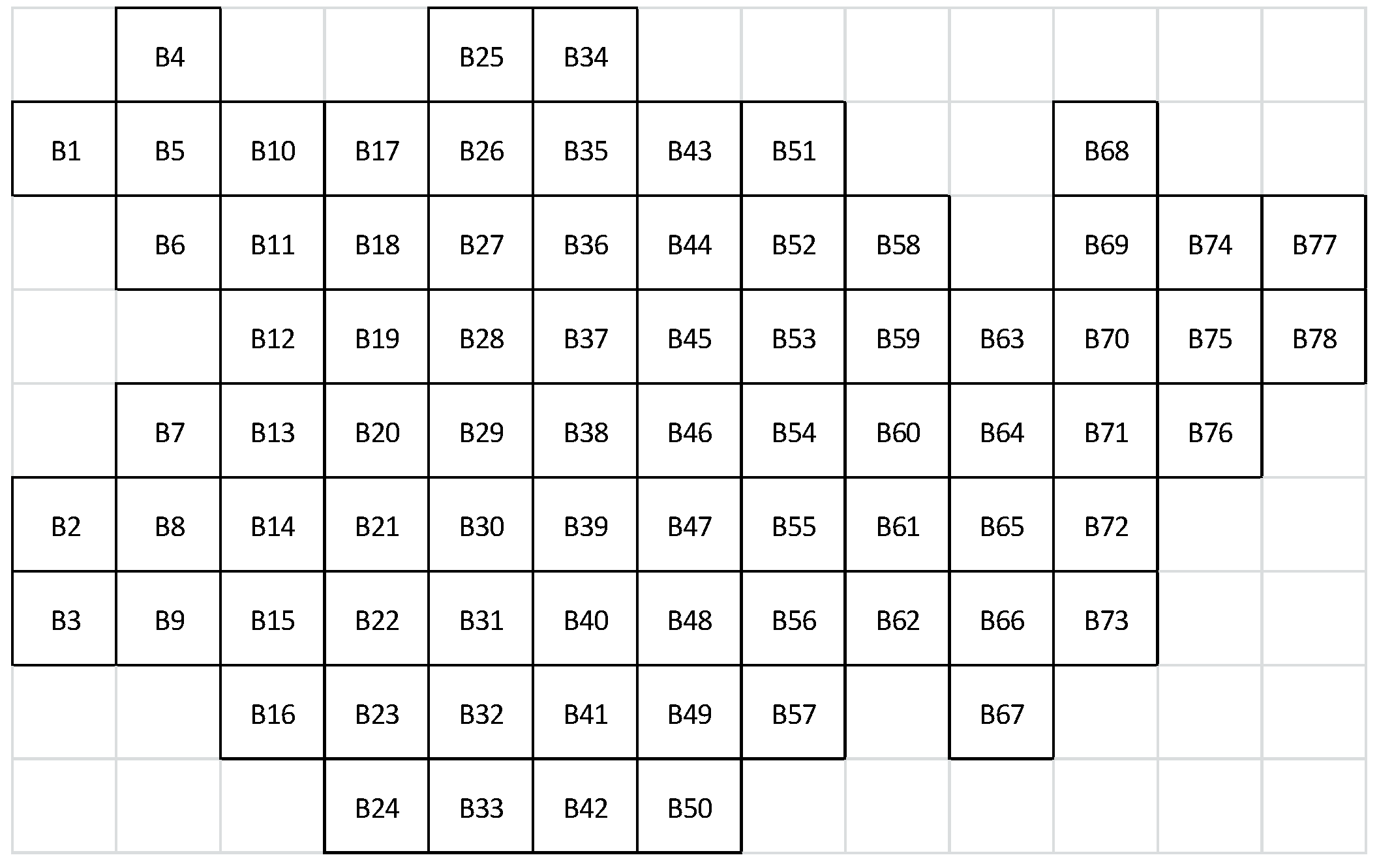
The traditional block model of coal deposit means the deposit is divided into an adequate number of blocks having the same size. Such a model is created using the data obtained from exploration drilling and application of geostatistical methods. Supposing what portion of the coal deposit is defined to be mineable in economical way (mineable reserves), i.e., the ultimate number of mineable blocks is defined.

Let $B={\left\{b_k\right\}}_{k\ge 1}$ be the set of mineable blocks in the coal deposit. Each block is characterized by a certain number of attributes, such as dimensions, location, density, tonnage, heating value, sulfur and ash content. Without loss of generality we suppose the density and tonnage are the same for every block. With respect to the thermal power plant’s requirements, heating value, sulfur and ash content are the main modeling attributes of. Such attributes are used to determine the possible technological value of every block in B.

One of methods of reducing the size of the production planning problem is to first combine all mineable blocks into block aggregates based on relative closeness of their attributes to the given technological requirements.

Definition 1.

Let ${\left\{b_k\right\}}_{k\ge 1}$ be a sequence of mineable blocks. A subsecuence of ${\left\{b_k\right\}}_{k\ge 1}$ is a sequence ${\left\{b_{k_i}\right\}}_{i\ge 1}$ with $k_i<k_{i+1}$ for all $i\ge 1$ [14].

Definition 2.

A point c is called a cluster point or accumulation point of a sequence ${\left\{b_k\right\}}_{k\ge 1}$ if for any $\epsilon >0$ and any $K\ge 1$ there is an $k\ge K$ such that $|c-b_k|<\epsilon$ [14].

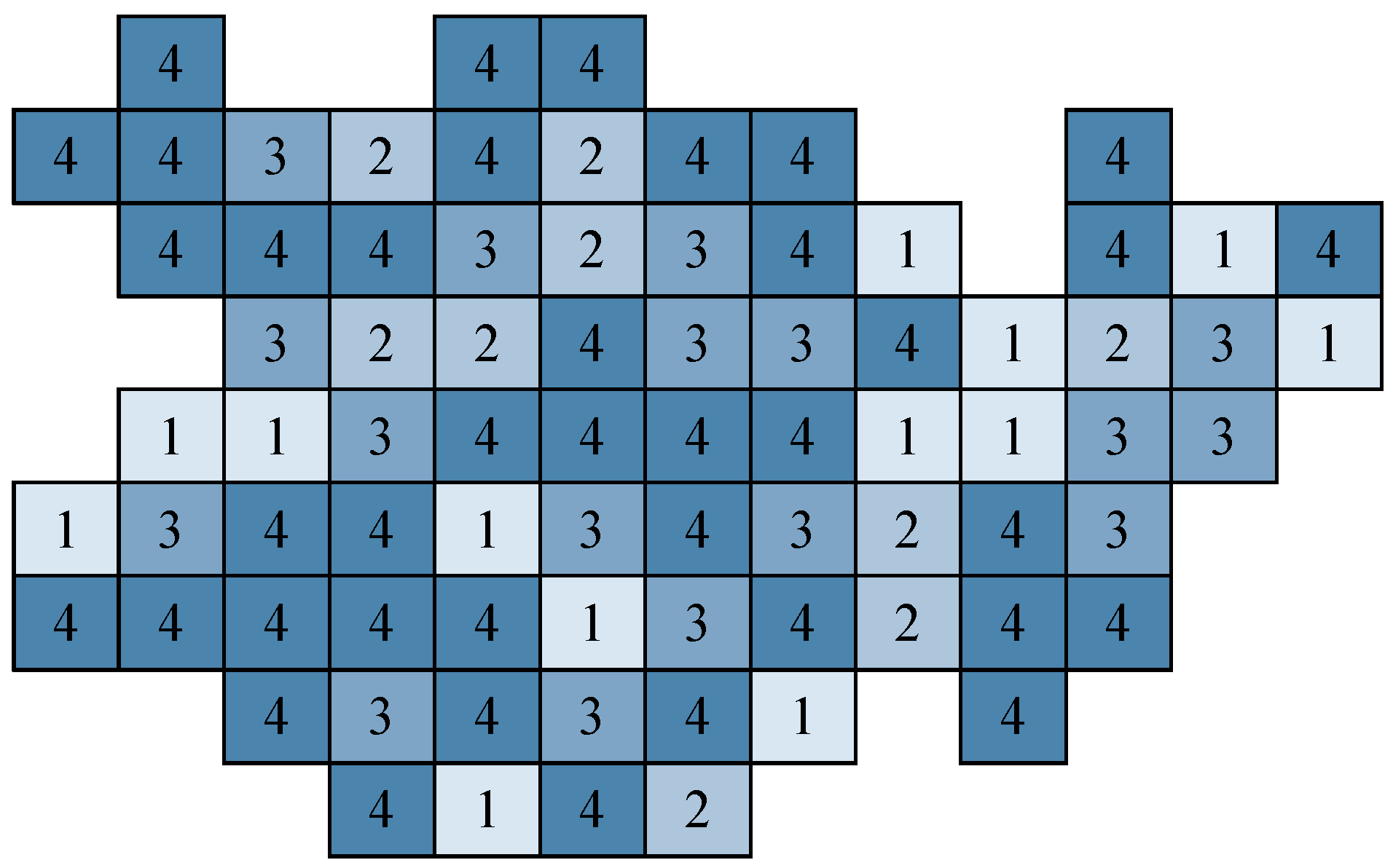
Considering Definitions 1 and 2 we can create cluster composed of mineable blocks. We refer to this cluster composed of blocks as a technological mining cut. Obviously, the mineable reserves can be represented by the set composed of all technological mining cuts. Formally, the clustering structure of the coal deposit is represented as a set of the following subsets $C=C_1,C_2,\dots ,C_n$ of $B={\left\{b_k\right\}}_{k\ge 1}$ such that: $B={{\displaystyle \cup }}_{n=1}^N{C}_n$ and $C_n{\displaystyle \cap }{C}_l=\varnothing$ for $m\ne l$. Consequently, any mineable block in B belongs to exactly one and only one technological mining cut.

Definition 3.

Let ${\tilde{B}}^{act}=\left\{{\tilde{b}}_i^{act}\right\}={\left\{{\tilde{h}}_i^{act},{\tilde{u}}_i^{act},{\tilde{p}}_i^{act}\right\}}_{i=1,2,\dots ,k}$ be a set of the triangular fuzzy numbers describing actual values of heating value, sulfur and ash content of the block respectively, where k is the total number of mineable blocks.

Definition 4.

Let ${\tilde{A}}^{tar}=\left\{{\tilde{h}}^{tar},{\tilde{u}}^{tar},{\tilde{p}}^{tar}\right\}$ be a set of the triangular fuzzy numbers describing the target values of attributes required by the thermal power plant.

Definition 5.

Let $\tilde{S}={\left\{{\tilde{s}}_i\right\}}_{i=1,2,\dots ,k}$ be a set of the triangular fuzzy numbers describing the relative closeness of every mineable block to the ${\tilde{A}}^{tar}$.

Considering Definitions 3–5 we can define technological mining cut (cluster) as a three attributes spatial object, composed of mineable blocks, with relative closeness belonging to one and only one predefined cluster interval. Therefore, the problem statement is to divide the area of the coal deposit into N technological mining cuts. The procedure of the solving the problem is divided into two main phases:

• calculation of the relative closeness of every mineable block to the target values based on the Technique for Order Preference by Similarity to the Ideal Solution (TOPSIS) method,
• clustering the obtained values based on the fuzzy C-mean clustering method.

2.2. The Relative Closeness

In order to define the relative closeness of block to the target values we apply the concept of multi-criteria decision making. To decrease the uncertainty of the input attributes we apply fuzzy set theory i.e., triangular fuzzy numbers [15,16]. Application of the fuzzy set theory has found wide use for solving problems in the mining industry [17,18,19,20,21].

Let X be a classical set of objects, called the universe, whose generic elements are denoted by x. The membership in a crisp subset X is often viewed as characteristic function ${\mu }_A$ from X to {0, 1} such that:

$${\mu }_A\left(x\right)=\{\begin{array}{l}1ifandonlyifx\in A,\hfill \\ 0otherwise\hfill \end{array},$$

(1)

where {0, 1} is called a valuation set. If the valuation set is allowed to be real interval [0, 1], A is called a fuzzy set and denoted by $\tilde{A}$ and ${\mu }_{\tilde{A}}\left(x\right)$ is the degree of membership of x in $\tilde{A}$.

A triangular fuzzy number is created according to probability-possibility transformation [22,23,24]. In order to calculate the relative closeness, ${\tilde{s}}_i=f\left({\tilde{b}}_i^{act},{\tilde{A}}^{tar}\right)$, between the i-th mineable block and requirements of the thermal power plant we apply the modified TOPSIS method. Modification refers primarily to the different sequence of steps and calculation of attribute weights than the ones used in the original method. The TOPSIS method is a technique for order preference by similarity to an ideal solution proposed by Hwang and Yoon (1981) [25]. The basic concept of this method is that the chosen alternative should have the shortest distance from the positive ideal solution and the farthest distance from the negative ideal solution.

Application of fuzzy TOPSIS can be found in many scientific papers. Chen [26] extended the use of TOPSIS to the fuzzy environment and gave numerical examples of system analysis engineer selection for a software company. Chu [27] presented a fuzzy TOPSIS model under group decisions for solving the facility location selection problem. Yang and Hung [28] proposed the use of TOPSIS and fuzzy TOPSIS methods for plant layout design problem.

The modified fuzzy TOPSIS method is based on the following steps:

Step 1: Normalization of the input data

The space of the input data is defined by the union of the mineable block attributes and target values. It can be represented by the following input data matrix:

$$\tilde{Y}=\left[\begin{array}{cccc}{\tilde{y}}_{11}^{act}& {\tilde{y}}_{12}^{act}& \cdots & {\tilde{y}}_{1j}^{act}\\ {\tilde{y}}_{21}^{act}& {\tilde{y}}_{22}^{act}& \cdots & {\tilde{y}}_{2j}^{act}\\ ⋮& ⋮& \ddots & ⋮\\ {\tilde{y}}_{i1}^{act}& {\tilde{y}}_{i2}^{act}& \cdots & {\tilde{y}}_{ij}^{act}\\ {\tilde{y}}_1^{tar}& {\tilde{y}}_2^{tar}& \cdots & {\tilde{y}}_j^{tar}\end{array}\right] i=1,2,\dots ,k;j=1,2,\dots ,m,$$

(2)

where k is the total number of the mineable blocks in the coal deposit and m is the total number of the attributes. In our case the input data matrix is as follows:

$$\tilde{D}=\left[\begin{array}{ccc}{\tilde{h}}_1^{act}& {\tilde{u}}_1^{act}& {\tilde{p}}_1^{act}\\ {\tilde{h}}_2^{act}& {\tilde{u}}_2^{act}& {\tilde{p}}_2^{act}\\ ⋮& ⋮& ⋮\\ {\tilde{h}}_i^{act}& {\tilde{u}}_i^{act}& {\tilde{p}}_i^{act}\\ {\tilde{h}}^{tar}& {\tilde{u}}^{tar}& {\tilde{p}}^{tar}\end{array}\right],$$

(3)

Note, in the input data matrix, requirement of the thermal power plant is treated as a fictitious mineable block. Each element of the matrix $\tilde{Y}$ is transformed using the following equations:

$${\tilde{r}}_{ij}=\frac{{\tilde{y}}_{ij}^{act}}{{{\displaystyle \sum }}_{i=1}^k{\tilde{y}}_{ij}^{act}+{\tilde{y}}_j^{tar}}=\frac{\left(a_{ij}^{act},b_{ij}^{act},c_{ij}^{act}\right)}{{{\displaystyle \sum }}_{i=1}^k\left(a_{ij}^{act},b_{ij}^{act},c_{ij}^{act}\right)+\left(a_j^{tar},b_j^{tar},c_j^{tar}\right) } j=1,2,\dots ,m,$$

(4)

$${\tilde{r}}_j=\frac{{\tilde{y}}_j^{tar}}{{{\displaystyle \sum }}_{i=1}^k{\tilde{y}}_{ij}^{act}+{\tilde{y}}_j^{tar}}=\frac{\left(a_j^{tar},b_j^{tar},c_j^{tar}\right)}{{{\displaystyle \sum }}_{i=1}^k\left(a_{ij}^{act},b_{ij}^{act},c_{ij}^{act}\right)+\left(a_j^{tar},b_j^{tar},c_j^{tar}\right) } j=1,2,\dots ,m,$$

(5)

Equation (4) refers to the block attributes while Equation (5) refers to the targets. The normalized input data matrix is as follows:

$$\tilde{R}=\left[\begin{array}{cccc}{\tilde{r}}_{11}& {\tilde{r}}_{12}& \cdots & {\tilde{r}}_{1j}\\ {\tilde{r}}_{21}& {\tilde{r}}_{22}& \cdots & {\tilde{r}}_{2j}\\ ⋮& ⋮& \ddots & ⋮\\ {\tilde{r}}_{i1}& {\tilde{r}}_{i2}& \cdots & {\tilde{r}}_{ij}\\ {\tilde{r}}_1& {\tilde{r}}_2& \cdots & {\tilde{r}}_j\end{array}\right] i=1,2,\dots ,k;j=1,2,\dots ,m,$$

(6)

Step 2: Weights of the attributes and targets

In the original TOPSIS method the global weight of each criterion is calculated, while in our model we calculate the local weight of each attribute within the mineable block and technological requirement (targets) separately. The weight of a block attribute is calculated as follows:

$${\tilde{w}}_{ij}=\frac{{\tilde{r}}_{ij}}{{{\displaystyle \sum }}_{j=1}^m{\tilde{r}}_{ij}}, {{\displaystyle \sum }}_{j=1}^m{\tilde{w}}_{ij}=1,i=1,2,\dots ,k,$$

(7)

The weight of target value is calculated as follows:

$${\tilde{w}}_j=\frac{1}{m}, {{\displaystyle \sum }}_{j=1}^m{\tilde{w}}_j=1,$$

(8)

The weights of target attributes are assumed to have equal importance.

Step 3: Construct the decision matrix

The first phase in solving the problem of the coal deposit partitioning into finite number of technological mining cuts can be treated as an Alternatives, Criteria, Evaluations model. A finite set of alternatives is defined by the set $B={\left\{b_k\right\}}_{k\ge 1}$, i.e., each mineable block represents one alternative. A finite set of criteria is defined by the set $F=\left\{f_1,f_2,\dots ,f_j\right\}$, where each element represents the distance function between the j-th block attribute and the j-th target value. A set of evaluations of alternatives with respect to given criteria is defined by the set $\tilde{X}=\left[{\tilde{x}}_{ij}\right]$, where each element represents the rating of the alternative with respect to defined criterion.

Heating value, sulfur and ash content are used as three main attributes in the calculation of distance functions, i.e., in the process of the block evaluation. Accordingly we have the set F composed of three basic distance functions, i.e., the set of criteria is defined as $F=\left\{f_1,f_2,f_3\right\}$. Evaluation of each element of the set $\tilde{X}$ is obtained as follows:

$${\tilde{x}}_{ij}=\frac{{\tilde{w}}_j{\tilde{r}}_j-{\tilde{w}}_{ij}{\tilde{r}}_{ij}}{{\tilde{w}}_j{\tilde{r}}_j} i=1,2,\mathrm{..},k, j=1,2,\mathrm{..},m,$$

(9)

where term ${\tilde{w}}_j{\tilde{r}}_j$ refers to the weighted normalized target value of the j-th attribute while ${\tilde{w}}_{ij}{\tilde{r}}_{ij}$ to the actual value of the mineable block.

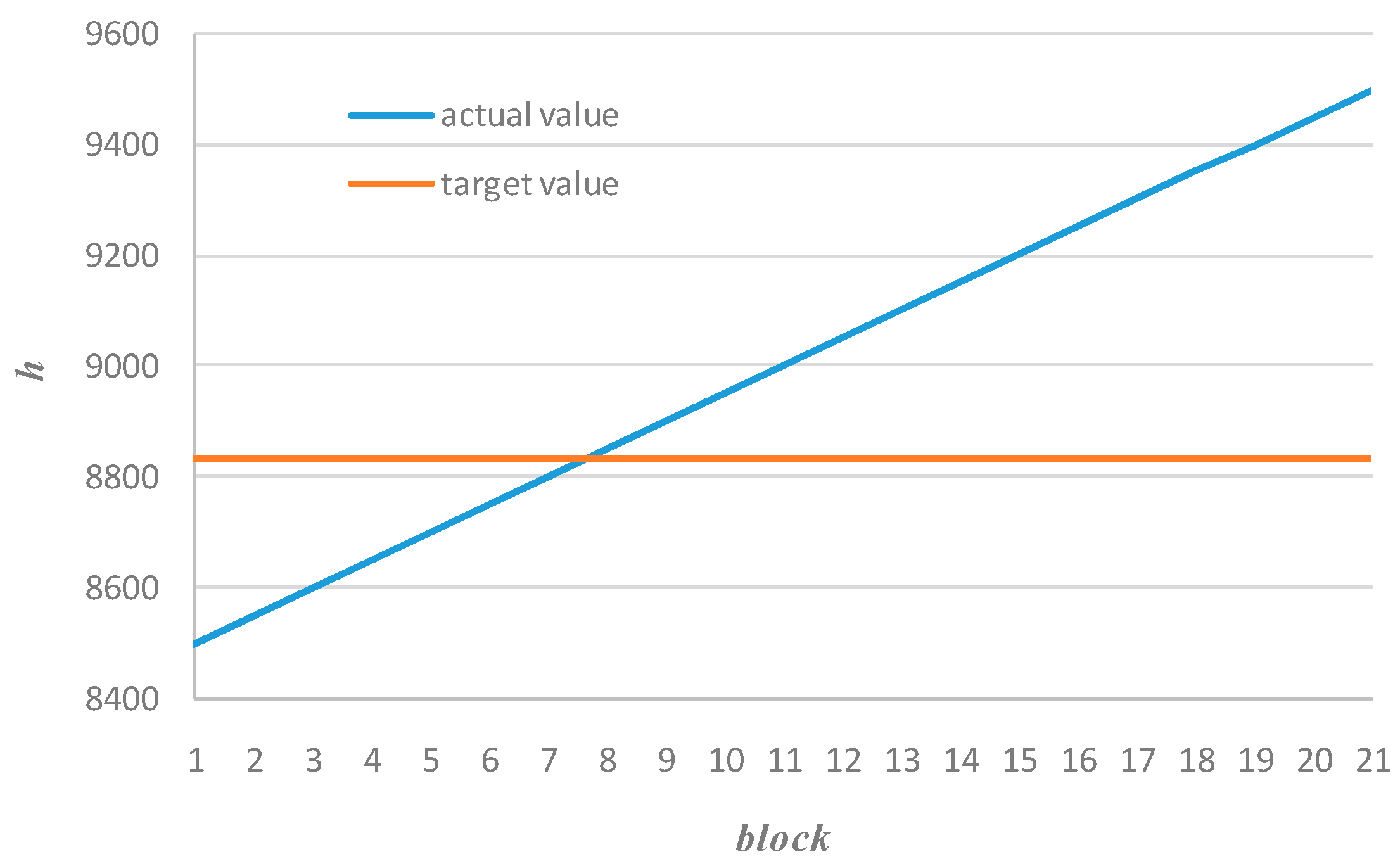
The criterion based on the heating value (f₁) is divided into two criteria with respect to the sign of the distance function (f₁ > 0; f₁ < 0). Suppose there is a sequence of mineable blocks with ascending order of the heating value and required (target) value, see Figure 1.

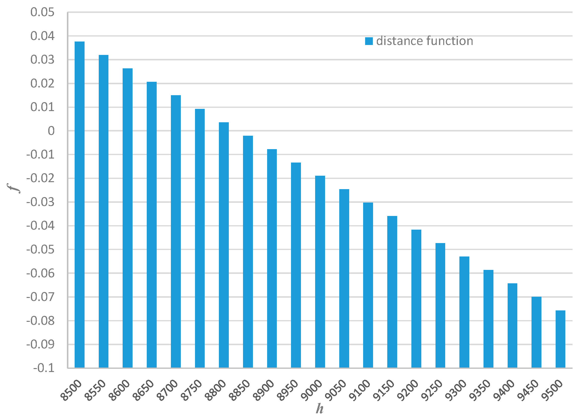
According to Equation (9) we obtain descending order of the distance function values, see Figure 2. The sign of the distance function is defined by the following sign function of f₁:

$$sign\left(f_{i1}\right)=\{\begin{array}{c}- if {\tilde{w}}_{i1}{\tilde{r}}_{i1}>{\tilde{w}}_1{\tilde{r}}_1\\ 0 if {\tilde{w}}_{i1}{\tilde{r}}_{i1}={\tilde{w}}_1{\tilde{r}}_1\\ + if {\tilde{w}}_{i1}{\tilde{r}}_{i1}<{\tilde{w}}_1{\tilde{r}}_1\end{array}, i=1,2,\dots ,k,$$

(10)

By the sign of the heating value distance function we generally separate the mineable blocks into two subsets, where the first subset is composed of the mineable blocks having a heating value greater than the target ($sign\left(f_{i1}\right)=-$), while the second are the blocks having a lower value ($sign\left(f_{i1}\right)=+$). Accordingly, we obtain the two following criteria $f_1^1$ and $f_1^2$. It is very important to emphasize that one and only one of these two criteria exists in the i-th mineable block. It is defined as follows:

$$f_{i1}^1=\{\begin{array}{c}1 if {\tilde{w}}_{i1}{\tilde{r}}_{i1}>{\tilde{w}}_1{\tilde{r}}_1 or sign\left(f_{i1}\right)=- \\ 0 if {\tilde{w}}_{i1}{\tilde{r}}_{i1}<{\tilde{w}}_1{\tilde{r}}_1 or sign\left(f_{i1}\right)=+\end{array}, i=1,2,\dots ,k,$$

(11)

$$f_{i1}^2=\{\begin{array}{c}1 if {\tilde{w}}_{i1}{\tilde{r}}_{i1}<{\tilde{w}}_1{\tilde{r}}_1 or sign\left(f_{i1}\right)=+\\ 0 if {\tilde{w}}_{i1}{\tilde{r}}_{i1}>{\tilde{w}}_1{\tilde{r}}_1 or sign\left(f_{i1}\right)=-\end{array}, i=1,2,\dots ,k,$$

(12)

Note, [0, 1] indicates only the existence of the criterion in the i-th mineable block not the evaluated values. Criterion $f_1^1$ should be maximized while $f_1^2$ is minimized. Accordingly, the set of criteria is transformed and is as follows; $F=\left\{f_1,f_2,f_2\to f_3,f_3\to f_4\right\}$. Evaluation of each element of the set $\tilde{X}$ with respect to criteria based on the sulfur and ash content (f₃, f₄) is also evaluated by Equation (11). Both criteria should be maximized. Finally we obtain the following decision matrix:

$$\tilde{X}={[{\tilde{x}}_{i4}]}_{k\times 4}=\left[\begin{array}{ccccc}B/F& f_1=f_1^1\to max& f_2=f_1^2\to min& f_3\to max& f_3\to max\\ b_1& {\tilde{x}}_{11}\in [0,1]& {\tilde{x}}_{12}\in [0,1]& {\tilde{x}}_{13}& {\tilde{x}}_{14}\\ b_2& {\tilde{x}}_{21}\in [0,1]& {\tilde{x}}_{22}\in [0,1]& {\tilde{x}}_{23}& {\tilde{x}}_{24}\\ ⋮& ⋮& ⋮& \ddots & ⋮\\ b_i& {\tilde{x}}_{i1}\in [0,1]& {\tilde{x}}_{i2}\in [0,1]& {\tilde{x}}_{i3}& {\tilde{x}}_{i4}\end{array}\right],$$

(13)

Step 4: Define the ideal and the negative-ideal solutions

Let us suppose that ${\tilde{A}}^{+}$ identifies the ideal solution and ${\tilde{A}}^{-}$ the negative one. They are defined as follows:

$${\tilde{A}}^{+}=\left\{\left(\underset{i=1,2,\mathrm{..},k}{\underbrace{max}}{\tilde{x}}_{ij}|j\in J\right),\left(\underset{i=1,2,\mathrm{..},k}{\underbrace{min}}{\tilde{x}}_{ij}|j\in J^{\prime }\right)\right\}=\left\{{\tilde{x}}_1^{+},{\tilde{x}}_2^{+},\dots ,{\tilde{x}}_m^{+}\right\},$$

(14)

$${\tilde{A}}^{-}=\left\{\left(\underset{i=1,2,\mathrm{..},k}{\underbrace{min}}{\tilde{x}}_{ij}|j\in J\right),\left(\underset{i=1,2,\mathrm{..},k}{\underbrace{max}}{\tilde{x}}_{ij}|j\in J^{\prime }\right)\right\}=\left\{{\tilde{x}}_1^{-},{\tilde{x}}_2^{-},\dots ,{\tilde{x}}_m^{-}\right\},$$

(15)

where:

J = {j = 1,2,...,m | j associated with the benefit criteria}

J’ = {j = 1,2,...,m | j associated with the cost criteria}

With benefit and cost attributes, we discriminate between criteria that the decision maker desires to maximize or minimize, respectively.

Step 5: Measure the distance between alternatives and ideal solutions

To calculate the m-Euclidean distance from each alternative (mineable block) to ${\tilde{A}}^{+}$ and ${\tilde{A}}^{-}$ the following equations can be easily adopted:

$${\tilde{s}}_i^{+}=\sqrt{{{\displaystyle \sum }}_{j=1}^m{\left({\tilde{x}}_{ij}-{\tilde{x}}_j^{+}\right)}^2 } i=1,2,\dots ,k,$$

(16)

$${\tilde{s}}_i^{-}=\sqrt{{{\displaystyle \sum }}_{j=1}^m{\left({\tilde{x}}_{ij}-{\tilde{x}}_j^{-}\right)}^2 } i=1,2,\dots ,k,$$

(17)

Step 6: Measure of the relative closeness to the ideal solution

The elements of the set $\tilde{S}={\left\{{\tilde{s}}_i\right\}}_{i=1,2,\dots ,k}$ are calculated by the following equation:

$${\tilde{s}}_i=\frac{{\tilde{s}}_i^{-}}{{\tilde{s}}_i^{+}+{\tilde{s}}_i^{-}},$$

(18)

A very important concept related to the applications of triangular fuzzy numbers is the process of defuzzification. It converts a triangular fuzzy number into a crisp value The most commonly used defuzzification method is the centroid defuzzification method, which is also known as center of gravity [29]. The defuzzification formula of triangular fuzzy numbers (a,b,c) is:

$${\overline{x}}_0\left(\tilde{A}\right)=\left(a+b+c\right)/3,$$

(19)

and it will be used to express the fuzzy relative closeness as crisp value. Finally, we obtain the set of the relative closeness $S={\left\{s_i\right\}}_{i=1,2,\dots ,k}$ that should be partitioned into adequate number of clusters.

Applying the same concept to the sulfur and ash content attribute we can obtain the following decision matrix:

$$\tilde{X}={[{\tilde{x}}_{i6}]}_{k\times 6}=\left[\begin{array}{ccccccc}B/F& f_1=f_1^1\to max& f_2=f_1^2\to min& f_3=f_3^1\to max& f_4=f_3^2\to max& f_5=f_4^1\to max& f_6=f_4^2\to max\\ b_1& {\tilde{x}}_{11}\in [0,1]& {\tilde{x}}_{12}\in [0,1]& {\tilde{x}}_{13}\in [0,1]& {\tilde{x}}_{14}\in [0,1]& {\tilde{x}}_{15}\in [0,1]& {\tilde{x}}_{16}\in [0,1]\\ b_2& {\tilde{x}}_{21}\in [0,1]& {\tilde{x}}_{22}\in [0,1]& {\tilde{x}}_{23}\in [0,1]& {\tilde{x}}_{24}\in [0,1]& {\tilde{x}}_{25}\in [0,1]& {\tilde{x}}_{26}\in [0,1]\\ ⋮& ⋮& ⋮& ⋮& ⋮& \ddots & ⋮\\ b_i& {\tilde{x}}_{i1}\in [0,1]& {\tilde{x}}_{i2}\in [0,1]& {\tilde{x}}_{i3}\in [0,1]& {\tilde{x}}_{i4}\in [0,1]& {\tilde{x}}_{i5}\in [0,1]& {\tilde{x}}_{i6}\in [0,1]\end{array}\right],$$

(20)

2.3. Coal Deposit Partitioning Model

In order to divide a coal deposit into an adequate number of technological mining cuts we apply the fuzzy C-mean clustering algorithm [30,31,32,33] over the set $S={\left\{s_i\right\}}_{i=1,2,\dots ,k}$.

Algorithm aims to determine cluster centers c_n(n = 1, 2, …, N) and fuzzy partition matrix U by minimizing the following function:

$$J=\left(U,c_1,c_2,\dots ,c_n,S\right)={{\displaystyle \sum }}_{n=1}^N{{\displaystyle \sum }}_{i=1}^k{u}_{ni}^{\omega }{\left(c_n-s_i\right)}^2,$$

(21)

subject to:

$${{\displaystyle \sum }}_{n=1}^N{u}_{ni}=1, i=1,2,\dots ,k,$$

(22)

$$0\le u_{ni}\le 1, n=1,2,\dots ,N, i=1,2,\dots ,k,$$

(23)

$$0<{{\displaystyle \sum }}_{i=1}^k{u}_{ni}<n, n=1,2,\dots ,N,$$

(24)

The exponent $\omega$ is used to adjust the weighting effect of membership values. A large $\omega$ will increase the fuzziness of the function J. The value of $\omega$ is often set to 2. Applying partial derivative to the function J with respect to variable $u_{ni}^{\omega }$ and $c_n$ the following update equations are obtained:

$$c_n=\frac{{{\displaystyle \sum }}_{i=1}^k{u}_{ni}^{\omega }{s}_i}{{{\displaystyle \sum }}_{i=1}^k{u}_{ni}^{\omega }},$$

(25)

$$u_{ni}=\frac{{\left(\frac{1}{|s_i-c_n|}\right)}^{\frac{1}{\omega -1}}}{{{\displaystyle \sum }}_{n=1}^N{\left(\frac{1}{|s_i-c_n|}\right)}^{\frac{1}{\omega -1}}},$$

(26)

Based on Equations (21)–(26) we describe the model to coal deposit partitioning into technological mining cuts as follows:

Step 1:

select an integer number of technological mining cuts i.e., clusters (N) and threshold value $\epsilon$; let ω = 2;

Step 2:

input a set of initial cluster centers $\left[c_1,c_2,\dots ,c_n\right]$, composed of the increasing order values randomly chosen from the interval $\left[min\left\{s_i\right\},max\left\{s_i\right\}\right], i=1,\mathrm{2..},k$;

Step 3:

compute all $\sqrt{{\left(c_n-s_i\right)}^2}$ and then all u_ni according to Equation (26);

Step 4:

update the set of initial cluster centers according to Equation (25);

Step 5:

compute the value of the objective function J according to Equation (21) and compare J^(t+1) with J^(t), where t is the iteration number. If $|J^{\left(t+1\right)}-J^{\left(t\right)}|<\epsilon$ then stop otherwise return to Step 2.

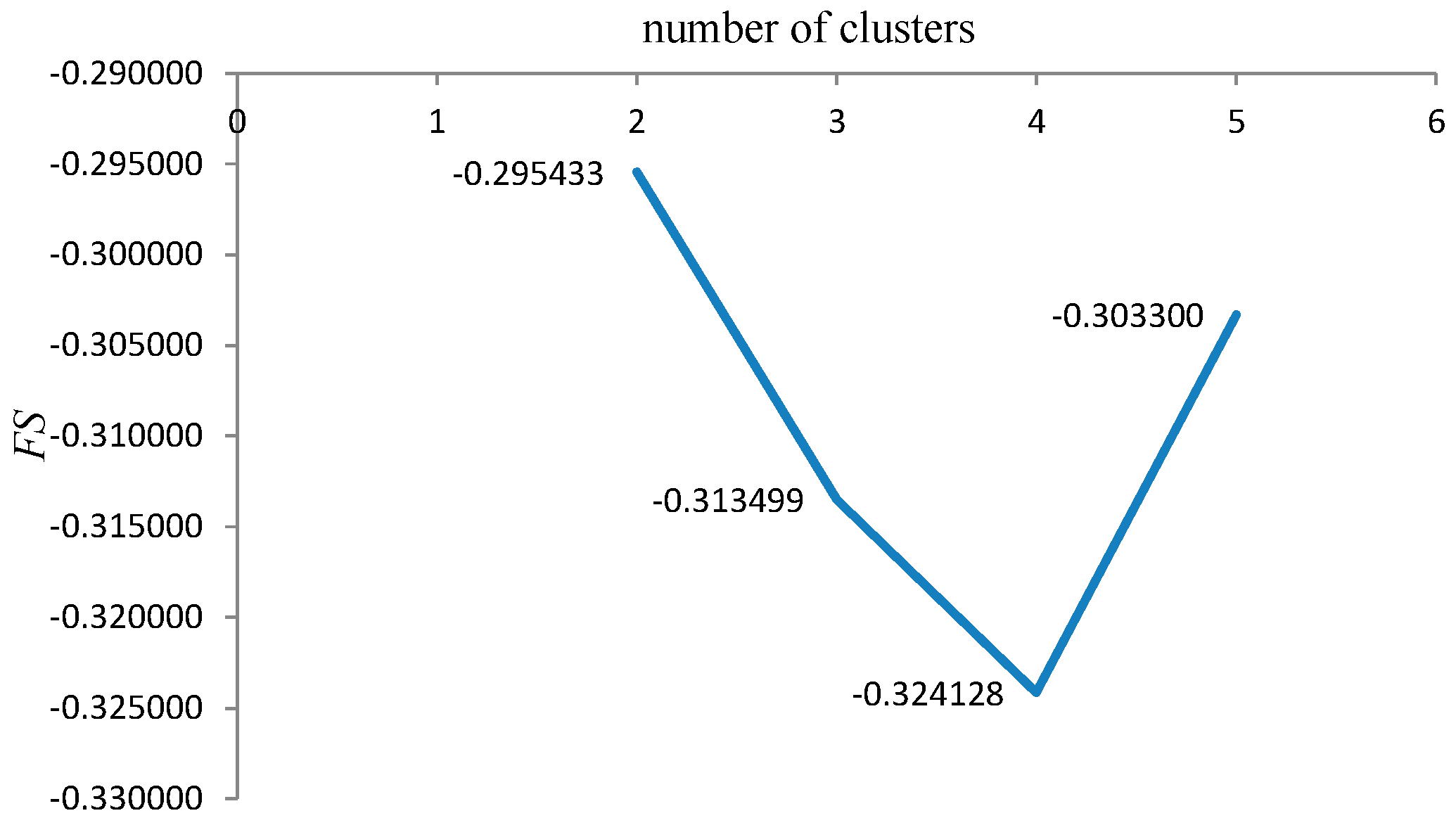
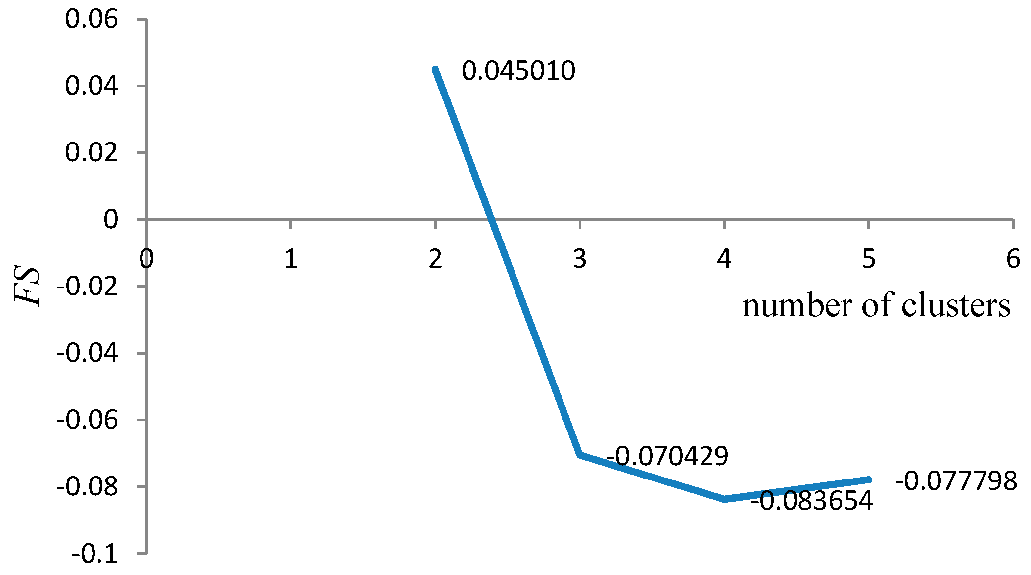
Determination of the optimal number of technological mining cuts (N) is based on the fuzzy validity criterion. The Fukuyama-Sugeno validity functional is used to define it [34,35,36]:

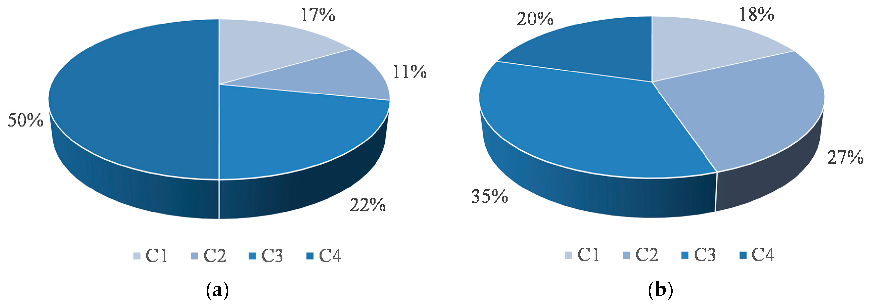
Since we have two clustering approaches based on four and six criteria, respectively, it is necessary to compare them. There are numerous measures for comparing clustering results. In this paper the adjusted Rand index (ARI) is used for comparison [37,38,39,40].

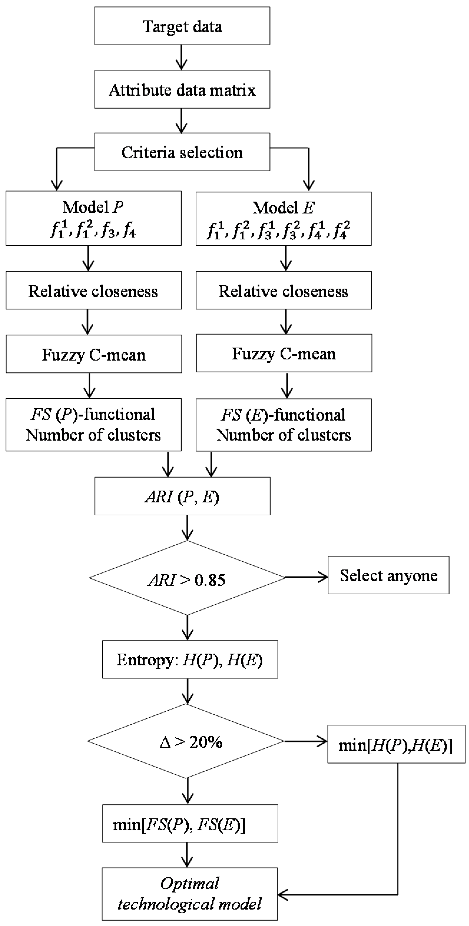
The range of ARI is $0\le ARI\le 1$, with only extreme values below zero. A value 0 indicates that there is no similarity, whereas a value of 1 indicates a similarity. If the value of ARI is high (ARI > 0.85) then mine production planners can select any one of the obtained models, otherwise it is necessary to select the optimal partitioning.

The selection is based on the entropy as a measure of quality of the obtained clusters [41,42]. This measure considers the overlaps between clusters P and E. The entropy of cluster P and E is H(P) and H(E). The optimal technological model of the coal deposit is selected according to: $min\left[H\left(P\right),H\left(E\right)\right]$. If there is no significant difference between H(P) and H(E), (<20%), then some additional way of selection have to be employed. For that purpose we can use Fukuyama-Sugeno validity functional (FS). For compact and well separated clusters it is expected small value of FS. Optimal technological model of coal deposit is selected according to: $min\left[FS\left(P\right),FS\left(E\right)\right]$. 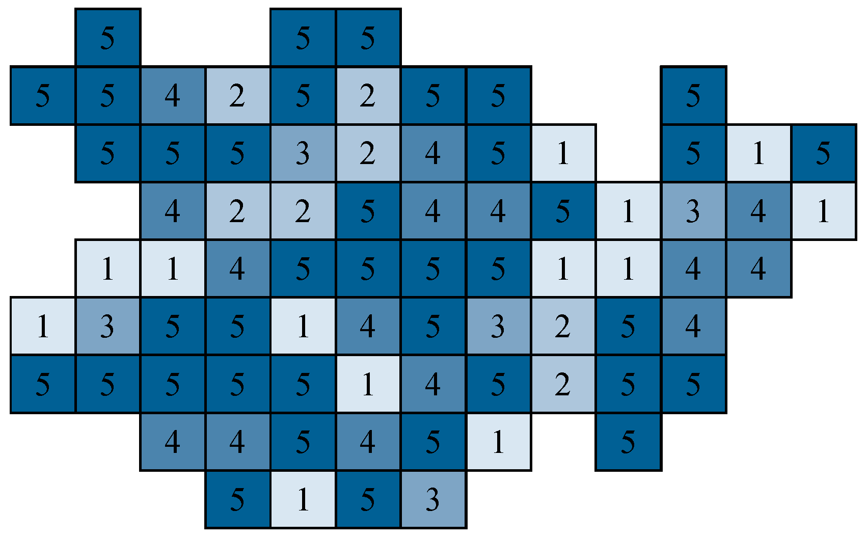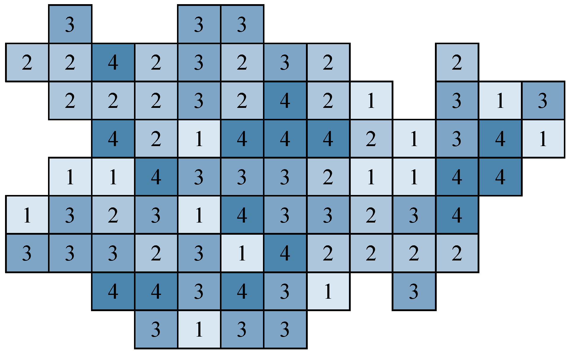A model of multi-attribute technological model of a coal deposit is represented in Figure 3.

3. Numerical Example

The developed model is tested on a small hypothetical coal deposit. A block model of the coal deposit was created on the basis of exploration drilling and geostatistical methods. The input parameters required for the model testing are given in Figure 4,

Table 1. Attributes of the mineable coal block.

Block	Heating Value (kJ/kg)			Sulfur (%)			Ash (%)			Block	Heating Value (kJ/kg)			Sulfur (%)			Ash (%)
1	8440.65	9378.50	10316.35	1.42	1.58	1.74	21.63	24.03	26.43	40	7338.38	8153.75	8969.13	1.61	1.79	1.96	24.45	27.17	29.88
2	7339.50	8155.00	8970.50	1.61	1.79	1.96	24.45	27.16	29.88	41	7928.10	8809.00	9689.90	1.51	1.68	1.84	22.94	25.49	28.04
3	8302.73	9225.25	10147.78	1.45	1.61	1.77	21.98	24.42	26.86	42	8298.00	9220.00	10142.00	1.45	1.61	1.77	21.99	24.44	26.88
4	8059.28	8954.75	9850.23	1.49	1.65	1.82	22.60	25.12	27.63	43	8059.05	8954.50	9849.95	1.49	1.65	1.82	22.60	25.12	27.63
5	8446.05	9384.50	10322.95	1.42	1.58	1.74	21.61	24.01	26.42	44	7814.48	8682.75	9551.03	1.53	1.70	1.87	23.23	25.81	28.39
6	8496.23	9440.25	10384.28	1.41	1.57	1.73	21.48	23.87	26.26	45	7881.75	8757.50	9633.25	1.52	1.68	1.85	23.06	25.62	28.18
7	7328.03	8142.25	8956.48	1.61	1.79	1.97	24.48	27.20	29.92	46	8073.45	8970.50	9867.55	1.48	1.65	1.81	22.57	25.08	27.58
8	7752.83	8614.25	9475.68	1.54	1.71	1.88	23.39	25.99	28.59	47	8237.48	9152.75	10068.03	1.46	1.62	1.78	22.15	24.61	27.07
9	8260.65	9178.50	10096.35	1.45	1.61	1.78	22.09	24.54	27.00	48	7917.53	8797.25	9676.98	1.51	1.68	1.85	22.97	25.52	28.07
10	7827.30	8697.00	9566.70	1.53	1.69	1.86	23.20	25.78	28.35	49	8177.63	9086.25	9994.88	1.47	1.63	1.79	22.30	24.78	27.26
11	8504.10	9449.00	10393.90	1.41	1.57	1.72	21.46	23.85	26.23	50	7709.18	8565.75	9422.33	1.55	1.72	1.89	23.50	26.11	28.72
12	7828.43	8698.25	9568.08	1.53	1.69	1.86	23.20	25.77	28.35	51	8378.33	9309.25	10240.18	1.43	1.59	1.75	21.79	24.21	26.63
13	7390.80	8212.00	9033.20	1.60	1.78	1.95	24.32	27.02	29.72	52	8415.00	9350.00	10285.00	1.43	1.58	1.74	21.69	24.10	26.51
14	8364.60	9294.00	10223.40	1.43	1.59	1.75	21.82	24.25	26.67	53	7890.08	8766.75	9643.43	1.51	1.68	1.85	23.04	25.60	28.16
15	8177.40	9086.00	9994.60	1.47	1.63	1.79	22.30	24.78	27.26	54	8494.43	9438.25	10382.08	1.41	1.57	1.73	21.49	23.88	26.26
16	7943.18	8825.75	9708.33	1.51	1.67	1.84	22.90	25.45	27.99	55	7746.08	8606.75	9467.43	1.54	1.71	1.88	23.41	26.01	28.61
17	7538.40	8376.00	9213.60	1.57	1.75	1.92	23.94	26.60	29.26	56	8512.43	9458.25	10404.08	1.41	1.57	1.72	21.44	23.83	26.21
18	8457.53	9397.25	10336.98	1.42	1.58	1.73	21.58	23.98	26.38	57	7334.55	8149.50	8964.45	1.61	1.79	1.97	24.46	27.18	29.90
19	7539.98	8377.75	9215.53	1.57	1.75	1.92	23.93	26.59	29.25	58	7255.58	8061.75	8867.93	1.63	1.81	1.99	24.30	27.00	29.70
20	7871.63	8746.25	9620.88	1.52	1.69	1.86	23.08	25.65	28.21	59	8372.93	9303.25	10233.58	1.43	1.59	1.75	21.80	24.22	26.65
21	8060.63	8956.25	9851.88	1.49	1.65	1.82	22.60	25.11	27.62	60	7354.58	8171.75	8988.93	1.60	1.78	1.96	24.41	27.12	29.83
22	8374.05	9304.50	10234.95	1.43	1.59	1.75	21.80	24.22	26.64	61	7630.20	8478.00	9325.80	1.56	1.73	1.90	23.70	26.34	28.97
23	7938.90	8821.00	9703.10	1.51	1.67	1.84	22.91	25.46	28.00	62	7576.65	8418.50	9260.35	1.57	1.74	1.92	23.84	26.49	29.14
24	8329.73	9255.25	10180.78	1.44	1.60	1.76	21.91	24.35	26.78	63	7299.00	8110.00	8921.00	1.61	1.79	1.97	24.55	27.28	30.01
25	8303.18	9225.75	10148.33	1.45	1.61	1.77	21.98	24.42	26.86	64	7261.65	8068.50	8875.35	1.62	1.80	1.98	24.65	27.39	30.13
26	8128.13	9031.25	9934.38	1.47	1.64	1.80	22.43	24.92	27.41	65	8215.20	9128.00	10040.80	1.46	1.62	1.78	22.20	24.67	27.14
27	7720.43	8578.25	9436.08	1.54	1.71	1.89	23.47	26.08	28.69	66	8488.58	9431.75	10374.93	1.41	1.57	1.73	21.50	23.89	26.28
28	7473.38	8303.75	9134.13	1.58	1.76	1.94	24.11	26.78	29.46	67	8082.23	8980.25	9878.28	1.48	1.65	1.81	22.55	25.05	27.56
29	8106.53	9007.25	9907.98	1.48	1.64	1.81	22.48	24.98	27.48	68	8502.53	9447.25	10391.98	1.41	1.57	1.73	21.47	23.85	26.24
30	7396.43	8218.25	9040.08	1.60	1.78	1.95	24.30	27.00	29.70	69	8256.38	9173.75	10091.13	1.45	1.61	1.78	22.10	24.55	27.01
31	8329.50	9255.00	10180.50	1.44	1.60	1.76	21.91	24.35	26.78	70	7704.00	8560.00	9416.00	1.55	1.72	1.89	23.51	26.13	28.74
32	8174.03	9082.25	9990.48	1.47	1.63	1.79	22.31	24.79	27.27	71	7906.73	8785.25	9663.78	1.51	1.68	1.85	23.00	25.55	28.11
33	7323.98	8137.75	8951.53	1.61	1.79	1.97	24.49	27.21	29.93	72	7907.85	8786.50	9665.15	1.51	1.68	1.85	22.99	25.55	28.10
34	8104.73	9005.25	9905.78	1.48	1.64	1.81	22.49	24.99	27.48	73	8406.90	9341.00	10275.10	1.43	1.59	1.74	21.71	24.13	26.54
35	7580.03	8422.25	9264.48	1.57	1.74	1.92	23.83	26.48	29.13	74	7394.18	8215.75	9037.33	1.60	1.78	1.95	24.31	27.01	29.71
36	7505.10	8339.00	9172.90	1.58	1.76	1.93	24.02	26.69	29.36	75	7868.03	8742.25	9616.48	1.52	1.69	1.86	23.09	25.66	28.23
37	7998.75	8887.50	9776.25	1.50	1.66	1.83	22.76	25.29	27.82	76	7858.80	8732.00	9605.20	1.52	1.69	1.86	23.12	25.69	28.26
38	8326.58	9251.75	10176.93	1.44	1.60	1.76	21.92	24.35	26.79	77	8165.03	9072.25	9979.48	1.47	1.63	1.79	22.33	24.81	27.30
39	7858.58	8731.75	9604.93	1.52	1.69	1.86	23.12	25.69	28.26	78	7410.15	8233.50	9056.85	1.60	1.77	1.95	24.27	26.96	29.66

and

Table 2. Input parameters.

Parameter	Value
Number of blocks	78
Block dimension	40 × 40 × 10 (m)
Target heating value	7494 8832 9715 (kJ/kg)
Target sulfur content	1.50 1.67 1.84 (%)
Target ash content	22.88 25.42 27.97 (%)
Number of technological mining-cuts	Fukuyama-Sugeno
The exponent $\omega$	2
Threshold value $\epsilon$	0.0001

.

Normalization of the input data is performed according to Equations (4) and (5). Calculation is presented only for the attributes of the first mineable block and target values as follows:

(1)

Heating value:

$${\tilde{r}}_{11}=\frac{\left(8440.65 9378.50 10316.35 \right)}{\left(620025 688917 757808\right)+\left(7494 8832 9715\right)}=\left(0.01100 0.01344 0.01644\right)$$

(27)

$${\tilde{r}}_1=\frac{\left(7494 8832 9715\right)}{\left(620025 688917 757808\right)+\left(7494 8832 9715\right)}=\left(0.00976 0.01266 0.01548\right)$$

(28)

(2)

Sulfur content:

$${\tilde{r}}_{12}=\frac{\left(1.42 1.58 1.74\right)}{\left(117.42 130.43 143.46\right)+\left(1.50 1.67 1.84\right)}=\left(0,0977 0.01196 0.01463\right)$$

(29)

$${\tilde{r}}_2=\frac{\left(1.50 1.67 1.84\right)}{\left(117.42 130.43 143.46\right)+\left(1.50 1.67 1.84\right)}=\left(0.01032 0.01264 0.01547\right)$$

(30)

(3)

ash content:

$${\tilde{r}}_{13}=\frac{\left(21.63 24.03 26.43\right)}{\left(1784.76 1983.12 2181.41 \right)+\left(22.88 25.42 27.97\right)}=\left(0.00979 0.01196 0.01462\right)$$

(31)

$${\tilde{r}}_3=\frac{\left(22.88 25.42 27.97\right)}{\left(1784.76 1983.12 2181.41 \right)+\left(22.88 25.42 27.97\right)}=\left(0.01036 0.01266 0.01547\right)$$

(32)

The weights of attributes of the first mineable block and target values are calculated as follows:

(1)

Heating value:

$${\tilde{w}}_{11}=\frac{\left(0.01100 0.01344 0.01644\right)}{\left(0.01100 0.01344 0.01644\right)+\left(0,0977 0.01196 0.01463\right)+\left(0.00979 0.01196 0.01462\right)}=\left(0.2406 0.3597 0.5379\right)$$

(33)

$${\tilde{w}}_1=\frac{1}{3}=0.3333$$

(34)

(2)

Sulfur content:

$${\tilde{w}}_{12}=\frac{\left(0,0977 0.01196 0.01463\right)}{\left(0.01100 0.01344 0.01644\right)+\left(0,0977 0.01196 0.01463\right)+\left(0.00979 0.01196 0.01462\right)}=\left(0.2138 0.3200 0.4787\right)$$

(35)

$${\tilde{w}}_2=\frac{1}{3}=0.3333$$

(36)

(3)

Ash content:

$${\tilde{w}}_{13}=\frac{\left(0.00979 0.01196 0.01462\right)}{\left(0.01100 0.01344 0.01644\right)+\left(0,0977 0.01196 0.01463\right)+\left(0.00979 0.01196 0.01462\right)}=\left(0.2142 0.3201 0.4784\right)$$

(37)

$${\tilde{w}}_3=\frac{1}{3}=0.3333$$

(38)

Distance functions of the first block are calculated as follows:

$${\tilde{x}}_{11}=\frac{0.3333·\left(0.00976 0.01266 0.01548\right)-\left(0.2406 0.3597 0.5379\right)·\left(0.01100 0.01344 0.01644\right)}{0.3333·\left(0.00976 0.01266 0.01548\right)}=\left(-1.0832 -0.1460 0.7722\right)$$

(39)

$${\tilde{x}}_{12}=\frac{0.3333·\left(0.01032 0.01264 0.01547\right)-\left(0.2138 0.3200 0.4787\right)·\left(0,0977 0.01196 0.01463\right)}{0.3333·\left(0.01032 0.01264 0.01547\right)}=\left(-0.6912 0.0913 0.8912\right)$$

(40)

$${\tilde{x}}_{13}=\frac{0.3333·\left(0.01036 0.01266 0.01547\right)-\left(0.2142 0.3201 0.4784\right)·\left(0.00979 0.01196 0.01462\right)}{0.3333·\left(0.01036 0.01266 0.01547\right)}=\left(-0.6871 0.0918 0.8864\right)$$

(41)

The sign of the heating value distance function of the first block is negative ($sign\left(f_{11}\right)=-$) and according to Equations (11) and (12) we obtain the following two criteria: $f_1^1=1$ and $f_1^2=0$. Finally, the input decision matrix is as follows:

$$\tilde{X}={[{\tilde{x}}_{i4}]}_{78\times 4}=\left[\begin{array}{ccccc}B/F& f_1=f_1^1\to max& f_2=f_1^2\to min& f_3\to max& f_4\to max\\ b_1& -1.0832-0.14600.7722& \times & -0.69120.09130.8912& -0.68710.09180.8864\\ b_2& \times & -0.59180.15570.9287& -1.0185-0.12990.7374& -1.0194-0.13050.7370\\ ⋮& ⋮& ⋮& \ddots & ⋮\\ b_{78}& \times & -0.61910.13750.9164& -0.9974-0.11580.7469& -0.9983-0.11640.7465\end{array}\right]$$

(42)

The set of the relative closeness $S={\left\{s_i\right\}}_{i=1,2,\dots ,78}$ is obtained by applying Equations (14)–(19) and represented in

Table 3. The relative closeness.

Block	$\tilde{\mathit{S}}={\left\{{\tilde{\mathit{s}}}_{\mathit{i}}\right\}}_{\mathit{i}=1,2,\dots ,78}$			Defuzzified	Block	$\tilde{\mathit{S}}={\left\{{\tilde{\mathit{s}}}_{\mathit{i}}\right\}}_{\mathit{i}=1,2,\dots ,78}$			Defuzzified
1	0.6014	0.6808	0.4539	0.5787	40	0.5243	0.1009	0.5204	0.3819
2	0.5244	0.1019	0.5203	0.3822	41	0.5689	0.6281	0.4794	0.5588
3	0.5935	0.7072	0.4598	0.5868	42	0.5932	0.7078	0.4600	0.5870
4	0.5780	0.6797	0.4720	0.5766	43	0.5780	0.6797	0.4720	0.5765
5	0.6017	0.6796	0.4537	0.5783	44	0.5607	0.5397	0.4864	0.5289
6	0.6043	0.6680	0.4517	0.5747	45	0.5656	0.5947	0.4822	0.5475
7	0.5235	0.0915	0.5212	0.3788	46	0.5789	0.6845	0.4712	0.5782
8	0.5562	0.4863	0.4904	0.5110	47	0.5895	0.7118	0.4628	0.5881
9	0.5910	0.7111	0.4617	0.5879	48	0.5682	0.6237	0.4801	0.5573
10	0.5617	0.5505	0.4856	0.5326	49	0.5858	0.7086	0.4657	0.5867
11	0.6047	0.6662	0.4514	0.5741	50	0.5529	0.4473	0.4933	0.4979
12	0.5618	0.5514	0.4855	0.5329	51	0.5979	0.6944	0.4564	0.5829
13	0.5284	0.1495	0.5163	0.3981	52	0.6000	0.6866	0.4549	0.5805
14	0.5971	0.6971	0.4570	0.5838	53	0.5662	0.6013	0.4817	0.5497
15	0.5857	0.7085	0.4658	0.5867	54	0.6042	0.6684	0.4518	0.5748
16	0.5700	0.6343	0.4786	0.5609	55	0.5557	0.4803	0.4909	0.5090
17	0.5399	0.2891	0.5052	0.4448	56	0.6052	0.6643	0.4511	0.5735
18	0.6023	0.6770	0.4532	0.5775	57	0.5240	0.0974	0.5207	0.3807
19	0.5401	0.2906	0.5051	0.4453	58	0.5213	0.0700	0.5234	0.3715
20	0.5649	0.5867	0.4829	0.5448	59	0.5976	0.6955	0.4567	0.5832
21	0.5781	0.6802	0.4719	0.5767	60	0.5256	0.1158	0.5192	0.3868
22	0.5977	0.6953	0.4566	0.5832	61	0.5470	0.3750	0.4987	0.4736
23	0.5697	0.6325	0.4788	0.5603	62	0.5429	0.3251	0.5025	0.4568
24	0.5951	0.7033	0.4585	0.5856	63	0.5212	0.0662	0.5236	0.3703
25	0.5935	0.7071	0.4597	0.5868	64	0.5183	0.0395	0.5266	0.3614
26	0.5826	0.6998	0.4683	0.5835	65	0.5881	0.7115	0.4639	0.5879
27	0.5538	0.4575	0.4926	0.5013	66	0.6039	0.6698	0.4520	0.5752
28	0.5349	0.2276	0.5100	0.4242	67	0.5795	0.6873	0.4707	0.5792
29	0.5811	0.6944	0.4694	0.5816	68	0.6046	0.6666	0.4515	0.5742
30	0.5289	0.1548	0.5159	0.3999	69	0.5907	0.7113	0.4619	0.5880
31	0.5951	0.7033	0.4586	0.5857	70	0.5526	0.4427	0.4937	0.4963
32	0.5855	0.7081	0.4659	0.5865	71	0.5674	0.6141	0.4807	0.5541
33	0.5232	0.0879	0.5216	0.3775	72	0.5675	0.6150	0.4807	0.5544
34	0.5810	0.6939	0.4695	0.5815	73	0.5995	0.6884	0.4552	0.5810
35	0.5431	0.3282	0.5022	0.4579	74	0.5287	0.1527	0.5161	0.3992
36	0.5374	0.2576	0.5077	0.4342	75	0.5646	0.5838	0.4831	0.5438
37	0.5738	0.6570	0.4753	0.5687	76	0.5640	0.5764	0.4836	0.5413
38	0.5949	0.7038	0.4587	0.5858	77	0.5849	0.7068	0.4664	0.5861
39	0.5639	0.5762	0.4837	0.5413	78	0.5300	0.1678	0.5148	0.4042

.

Calculation of the optimal number of technological mining cuts based on the Fukuyama-Sugeno validity functional is represented for the case of four criteria and five cluster centers. The set of initial cluster centers is [c₁, c₂, c₃, c₄, c₅] = [0.38, 0.42, 0.46, 0.50, 0.54]. Calculation of the first block membership degree indicating with what degree the relative closeness s₁ belongs to the initial cluster center vector [0.38, 0.42, 0.46, 0.50, 0.54] is represented in

Table 4. Membership degree of the first block to the initial cluster center vector.

	Euclidean Distance
s1 = 0.5787	0.38	0.42	0.46	0.50	0.54
	0.1987	0.1587	0.1187	0.0787	0.0387
Ω = 2	Membership degree
	c1 = 1	c2 = 2	c3 = 3	c4 = 4	c5 = 5
un1	0.086304	0.108058	0.144476	0.21792	0.443242
b1$\in$	No	No	No	No	Yes

.

The process of updating the cluster center vector is represented in

Table 5. Updating the cluster center vector.

Cn/Iteration	1	2	3	4	…	9
c1	0.38	0.38985	0.38975	0.38792	…	0.38439
c2	0.42	0.45535	0.46002	0.45586	…	0.44558
c3	0.46	0.49075	0.51084	0.51148	…	0.50674
c4	0.50	0.53099	0.54596	0.54964	…	0.55016
c5	0.54	0.56212	0.57287	0.57816	…	0.58086
J(t)	0.068953	0.029840	0.016992	0.012897	…	0.010989
$\epsilon$		0.039112	0.012848	0.004094	…	0.000054

.

After nine iterations threshold requirement is satisfied and technological model of coal deposit for matrix (78 × 4) and five cluster centers is obtained, see Figure 5.

Fuzzy characteristics of obtained technological mining cuts (clusters) are represented in

Table 6. Cluster’s fuzzy characteristics for a (78 × 4) matrix.

Cluster	Number of Blocks	Heating Value (kJ/kg)		Sulfur Content (%)		Ash Content (%)
		min	max	min	max	min	max
c1	13	7255.5 8061.7 8867.9	7410.1 8233.5 9056.8	1.59 1.77 1.95	1.62 1.81 1.99	24.26 26.96 29.66	24.64 27.38 30.12
c2	7	7473.3 8303.7 9134.1	7630.2 8478.0 9325.8	1.55 1.73 1.90	1.58 1.76 1.93	23.70 26.33 28.97	24.10 26.78 29.46
c3	5	7704.0 8560.0 9416.0	7752.8 8614.3 9475.7	1.54 1.71 1.88	1.55 1.72 1.89	23.39 25.99 28.59	23.51 26.12 28.73
c4	15	7814.5 8682.8 9551.0	7943.1 8825.7 9708.3	1.50 1.67 1.84	1.53 1.70 1.87	22.90 25.44 27.99	23.23 25.81 28.39
c5	38	7998.7 8887.5 9776.2	8512.4 9458.2 10404.0	1.41 1.56 1.72	1.49 1.66 1.82	21.44 23.82 26.20	22.75 25.28 27.81

.

The Fukuyama-Sugeno validity functional was analyzed for values of N between 2 and 5 and the obtained results are represented by Figure 6.

The optimal number of technological mining cuts is 4 and the technological model of the coal deposit composed of four mining cuts is represented by Figure 7.

According to Equation (20) the input decision matrix composed of six criteria is as follows:

$$\tilde{X}={[{\tilde{x}}_{i6}]}_{78\times 6}=\left[\begin{array}{ccccccc}B/F& f_1=f_1^1\to max& f_2=f_1^2\to min& f_3=f_3^1\to max& f_4=f_3^2\to max& f_5=f_4^1\to max& f_6=f_4^2\to max\\ & -1.0832& \times & \times & -0.6912& \times & -0.6871\\ b_1& -0.1460& \times & \times & 0.0913& \times & 0.0918\\ & 0.7722\ast & \times & \times & 0.8912& \times & 0.8864\\ & \times & -0.5918& -1.0185& \times & -1.0194& \times \\ b_2& \times & 0.1557& -0.1299& \times & -0.1305& \times \\ & \times & 0.9287& 0.7374& \times & 0.7370& \times \\ ⋮& ⋮& ⋮& ⋮& ⋮& \ddots & ⋮\\ & \times & -0.6191& -0.9974& \times & -0.9983& \times \\ b_{78}& \times & 0.1375& -0.1158& \times & -0.1164& \times \\ & \times & 0.9164& 0.7469& \times & 0.7465& \times \end{array}\right]$$

(43)

Triangular fuzzy number is represented in the vertical form (*). The set of the relative closeness $S={\left\{s_i\right\}}_{i=1,2,\dots ,78}$ is obtained by applying Equations (14)–(19) and represented in

Table 7. The relative closeness of the matrix (78 × 6).

Block	$\tilde{\mathit{S}}={\left\{{\tilde{\mathit{s}}}_{\mathit{i}}\right\}}_{\mathit{i}=1,2,\dots ,78}$			Defuzzified	Block	$\tilde{\mathit{S}}={\left\{{\tilde{\mathit{s}}}_{\mathit{i}}\right\}}_{\mathit{i}=1,2,\dots ,78}$			Defuzzified
1	0.5779	0.6534	0.4826	0.5713	40	0.5504	0.4781	0.5087	0.5124
2	0.5505	0.4787	0.5086	0.5125	41	0.5734	0.9456	0.4872	0.6687
$⋮$		$⋮$		$⋮$			$⋮$		$⋮$
39	0.5716	0.8878	0.4889	0.6494	78	0.5540	0.5156	0.5052	0.5249

.

The same procedure is performed for the input decision matrix (78 × 6). Fukuyama-Sugeno validity functional was analyzed for values of N between 2 and 5 and obtained results are represented by Figure 8.

The optimal number of technological mining cuts is four and the technological model of coal deposit composed of four mining cuts is represented by Figure 9.

4. Discussion

Table 8. Summary statistics of clusters for the matrix (78 × 4) and (78 × 6).

Cluster	Parameter	Number of Blocks	Heating Value (kJ/kg)	Sulfur Content (%)	Ash Content (%)	Number of Blocks	Heating Value (kJ/kg)	Sulfur Content (%)	Ash Content (%)
c1	min	13	8061.7	1.77	26.96	14	8061.7	1.76	26.78
	max		8233.5	1.81	27.38		8303.7	1.81	27.39
	expected		8156.1	1.79	27.13		8166.7	1.78	27.10
	standard deviation		54.8	0.01	0.12		65.8	0.01	0.15
	coefficient of variation (%)		0.67	0.59	0.46		0.81	0.68	0.56
c2	min	9	8303.7	1.71	26.11	21	8339.0	1.56	23.83
	max		8565.7	1.76	26.78		9458.3	1.75	26.69
	expected		8426.8	1.74	26.46		9101.8	1.63	24.73
	standard deviation		91.92	0.02	0.23		457.0	0.08	1.17
	coefficient of variation (%)		1.09	0.89	0.89		5.1	4.73	4.73
c3	min	17	8578.3	1.67	25.45	27	8560.0	1.60	24.34
	max		8821.0	1.72	26.08		9255.2	1.71	26.12
	expected		8726.6	1.68	25.70		9006.5	1.64	24.98
	standard deviation		72.28	0.01	0.18		227.3	0.04	0.58
	coefficient of variation (%)		0.82	0.72	0.72		2.5	2.33	2.33
c4	min	39	8825.7	1.56	23.82	16	8682.8	1.66	25.28
	max		9458.2	1.67	25.44		8887.5	1.69	25.81
	expected		9197.3	1.61	24.49		8766.6	1.68	25.59
	standard deviation		180.9	0.03	0.46		54.5	0.01	0.14
	coefficient of variation (%)		1.96	1.89	1.89		0.62	0.54	0.55

summarizes the characteristics of the two models obtained with respect to technological requirements and two sets composed of four and six criteria, respectively.

Distribution of the technological mining cuts with respect to defined technological requirements is represented by Figure 10.

Technological models of the coal deposit obtained for the input data matrices (78 × 4) and (78 × 6) are denoted by P and E, respectively. The information on the overlap between P and E is summarized in form of the following P × E confusion matrix:

$$V=\left[\begin{array}{cccccc}PartitionP\backslash Partition E& e_1& e_2& e_3& e_4& Sums\\ p_1& 13& 0& 0& 0& v_{1.}=13\\ p_2& 1& 6& 2& 0& v_{2.}=9\\ p_3& 0& 0& 3& 14& v_{3.}=17\\ p_4& 0& 15& 22& 2& v_{4.}=39\\ Sums& v_{.1}=14& v_{.2}=21& v_{.3}=27& v_{.4}=16& v_{..}=78\end{array}\right]$$

(44)

The elements of the alternative matrix (AV) are calculated using the values of elements of the matrix V as follows:

$$a={{\displaystyle \sum }}_{i=1}^4{{\displaystyle \sum }}_{j=1}^4\left(\begin{array}{c}{v}_{ij}\\ 2\end{array}\right)=\left(\begin{array}{c}13\\ 2\end{array}\right)+\left(\begin{array}{c}0\\ 2\end{array}\right)+\cdots +\left(\begin{array}{c}2\\ 2\end{array}\right)=525$$

(45)

$$b={{\displaystyle \sum }}_{i=1}^4\left(\begin{array}{c}{v}_{i.}\\ 2\end{array}\right)-a=\left(\begin{array}{c}13\\ 2\end{array}\right)+\left(\begin{array}{c}9\\ 2\end{array}\right)+\left(\begin{array}{c}17\\ 2\end{array}\right)+\left(\begin{array}{c}39\\ 2\end{array}\right)-525=466$$

(46)

$$c={{\displaystyle \sum }}_{j=1}^4\left(\begin{array}{c}{v}_{.j}\\ 2\end{array}\right)-a=\left(\begin{array}{c}14\\ 2\end{array}\right)+\left(\begin{array}{c}21\\ 2\end{array}\right)+\left(\begin{array}{c}27\\ 2\end{array}\right)+\left(\begin{array}{c}16\\ 2\end{array}\right)-525=247$$

(47)

$$d=\left(\begin{array}{c}k\\ 2\end{array}\right)-a-b-c=\left(\begin{array}{c}78\\ 2\end{array}\right)-525-466-247=1765$$

(48)

Alternative matrix is as follows:

$$AV=\left[\begin{array}{ccc}Model P\backslash Model E& Pair in same cut& Pair in different cuts\\ Pair in same cut& 525& 466\\ Pair in different cuts& 247& 1765\end{array}\right]$$

(49)

The adjusted Rand index (ARI) as the index of choice agreement between two technological models of coal deposit is:

$$ARI=\frac{\left(\begin{array}{c}78\\ 2\end{array}\right)\left(525+1765\right)-\left[\left(525+466\right)\left(525+247\right)+\left(247+1765\right)\left(466+1765\right)\right]}{{\left(\begin{array}{c}78\\ 2\end{array}\right)}^2-\left[\left(525+465\right)\left(525+247\right)+\left(247+1765\right)\left(466+1765\right)\right]}=0.431$$

(50)

The value of ARI indicates there is no high degree of agreement between two obtained technological models. The entropy of model P and E is calculated as follows:

$$H\left(P\right)=-{{\displaystyle \sum }}_{i=1}^4\frac{v_{i.}}{k}log\left(\frac{v_{i.}}{k}\right)=-\left[\frac{13}{78}log\left(\frac{13}{78}\right)+\frac{9}{78}log\left(\frac{9}{78}\right)+\frac{17}{78}log\left(\frac{17}{78}\right)+\frac{39}{78}log\left(\frac{39}{78}\right)\right]=0.5326$$

(51)

$$H\left(E\right)=-{{\displaystyle \sum }}_{j=1}^4\frac{v_{.j}}{k}log\left(\frac{v_{.j}}{k}\right)=-\left[\frac{13}{78}log\left(\frac{13}{78}\right)+\frac{9}{78}log\left(\frac{9}{78}\right)+\frac{17}{78}log\left(\frac{17}{78}\right)+\frac{39}{78}log\left(\frac{39}{78}\right)\right]=0.5879$$

(52)

According to: $min\left[H\left(P\right),H\left(E\right)\right]=min\left[0.5326,0.5879\right]=0.5326$, the optimal technological model of coal deposit is model P. Since the values of H(P) and H(E) are very similar we used the FS validity functional as additional way of selection.

According to: $min\left[FS\left(P\right),FS\left(E\right)\right]=min\left[-0.324128,-0.083654\right]=-0.083654$, the optimal technological model of coal deposit is also model P (see Figure 7).

5. Conclusions

Having the ability to make flexible production plans is recognized as a crucial element for the long term success of any mining company, especially in the coal sector. The efficiency of a plan depends directly on the quality of the input data. For that purpose we have developed the technological model of coal deposits to help mining engineers create production plans in an easier way. In nature this model is heterogeneous because the characteristic technological mining cuts can be located at different parts of the coal deposit. This means the cut is not continuous. Future research will be focused on the possibility of creation of a homogeneous model where each technological mining cut is continuous.